CIRCUMVENTING THE SIGN PROBLEM IN ROTATING QUANTUM MATTER
Casey Elizabeth Anderson Berger
A dissertation submitted to the faculty at the University of North Carolina at Chapel Hill in partial fulfillment of the requirements for the degree of Doctor of Philosophy in the Department of Physics and
Astronomy in the College of Arts and Sciences.
Chapel Hill 2020
© 2020
ABSTRACT
Casey Elizabeth Anderson Berger: Circumventing the Sign Problem in Rotating Superfluids Using Complex Langevin
(Under the direction of Joaquín E. Drut)
Quantum field theories with a complex action suffer from a sign problem in stochastic nonperturbative treatments, making many systems of great interest – such as polarized or mass-imbalanced fermions and QCD at finite baryon density – extremely challenging to treat numerically. Another such system is that of bosons at finite angular momentum; experimentalists have successfully achieved vortex formation in supercooled bosonic atoms, and have measured quantities of interest such as the moment of inertia. However, the rotation results in a complex action, making the usual numerical treatments of the theory unusable.
This thesis treats systems of nonrelativistic bosons with finite angular momentum using two approaches. One approach is to determine the virial coefficients using a semi-classical lattice approximation (SCLA). Through this approach, we are able to compute the thermodynamic equation of state of the bosons for finite trapping frequency, rotation, and inter-particle interaction. The second approach uses the complex Langevin (CL) method – a method which employs an extension of the Langevin equation to complex space and circumvents the sign problem to compute the full quantum behavior of a low energy system of interacting, trapped, and rotating bosons.
ACKNOWLEDGEMENTS
I was fortunate to have a strong support system to see me through my doctoral degree. Foremost, I am grateful for the financial and professional support of two wonderful and unique fellowship programs. The Department of Energy’s Computational Science Graduate Fellowship and UNC’s Royster Society of Fellows provided not just financial support but two active and vibrant communities of interdisciplinary scholars which became the twin pillars of my doctoral community. I can’t thank enough the incredible teams at the Krell Institute and UNC’s Graduate School who made sure fellows were able to take full advantage of the opportunities these programs provide. In particular, the two Royster Professors I had the privilege of working with, Professor Marsha Collins and Professor Banu Gökarıksel, both helped me take on leadership roles and become a better teacher, communicator, and colleague.
A few of my colleagues deserve special mention. Jessie: for the weekly lunches and coffee dates, your moral support and encouragement, and your unfailing reminders that we are more than the data we produce. Lukas: for all the enlightening discussions of theory and practical matters in computation, your consistent and infectious enthusiasm, and your thorough feedback on the dissertation which helped me produce a much better final draft. Lauren: for taking me under your wing when I was a confused undergraduate at my first conference, your steady wisdom and outside perspective, and your confidence in my ability to persevere. Jay: for your constant willingness to help, your mentorship in the earliest days of my research career, and your unending thoughtfulness. Emily: for being right there with me through the final push, for giving me snacks and a space to produce my first full draft, and for giving me a much-needed window into the world outside science.
I am lucky to have a loving and supportive family, both of the blood relative variety and the kind we choose for ourselves. Katie, Mary Beth, and Larkin, who have been there through my best days and my worst ones. Joe, who keeps me from taking myself too seriously. Liz, who didn’t get to see me make it to the end of this journey, but whose memory gives me strength. The Baumanns, who adopted me wholeheartedly and enrich my life in more ways than I can count. The Bergers: Mom, Dad, Michael, and Alannah, who have been on this journey with me, whether they liked it or not, and I’m thankful to have all of their support and love.
TABLE OF CONTENTS
LIST OF FIGURES . . . ix
LIST OF TABLES . . . xi
LIST OF ABBREVIATIONS . . . xii
LIST OF SYMBOLS . . . xiii
1 Introduction . . . 1
1.1 From two- to many-body systems . . . 1
1.1.1 The classical N-body problem . . . 1
1.1.2 The quantum N-body problem . . . 2
1.2 Stochastic methods and the sign problem . . . 5
1.2.1 The sign problem in quantum many-body physics . . . 6
1.3 Superfluidity . . . 7
1.4 Superfluids and rotation . . . 9
1.5 Outline . . . 10
2 Semi-classical lattice approximation for trapped, rotating, interacting quantum matter . . . 11
2.1 Motivation: why use a semi-classical lattice approximation? . . . 11
2.2 Hamiltonian and formalism . . . 11
2.2.1 Thermodynamics and the virial expansion . . . 12
2.2.2 Semiclassical lattice approximation . . . 14
2.2.3 Gauss-Hermite quadrature . . . 20
2.3 Results . . . 20
2.3.1 Noninteracting virial coefficients at finite angular momentum . . . 20
2.3.3 Interacting virial coefficients at finite angular momentum . . . 23
2.3.4 Interacting thermodynamics at finite angular momentum . . . 25
2.4 Summary and conclusions . . . 27
3 Stochastic methods: from Markov chain Monte Carlo to Complex Langevin. . . 28
3.1 Quantum Monte Carlo methods . . . 28
3.1.1 Importance sampling and the Ising model . . . 29
3.1.2 Limitations of quantum Monte Carlo algorithms . . . 31
3.2 Complex Langevin: origins and method . . . 31
3.2.1 Stochastic quantization: the Langevin method . . . 32
3.2.2 Extending the Langevin method to complex variables . . . 37
3.3 Formal justification and challenges for complex Langevin . . . 40
3.3.1 Mathematical aspects: convergence, correctness, boundary terms, and ergodicity . . 40
3.3.2 Practical aspects: numerical instabilities, gauge cooling, dynamic stabilization, and regulators . . . 44
4 The relativistic Bose gas . . . 46
4.1 Motivation . . . 46
4.2 Action and formalism: relativistic, interacting bosons at finite chemical potential . . . 46
4.3 Results . . . 49
4.3.1 Statistical and systematic effects . . . 49
4.3.2 The noninteracting case . . . 50
4.3.3 Real initialization, no interaction, zero chemical potential . . . 51
4.3.4 Finite chemical potential and interaction: the full CL treatment . . . 52
4.4 Summary and conclusions . . . 52
5 Interacting Bose gas at finite chemical potential and angular momentum . . . 54
5.1 Motivation . . . 54
5.2 Action and formalism . . . 54
5.3 The complex Langevin method for rotating bosons . . . 56
5.3.2 Calculating observables . . . 58
5.4 Results . . . 59
5.4.1 The free Bose gas . . . 59
5.4.2 The trapped, rotating, interacting Bose gas . . . 60
5.5 Summary and conclusions . . . 62
6 Discussion and Conclusion . . . 64
APPENDIX A DERIVATIONS FOR CALCULATING VIRIAL COEFFICIENTS . . . 66
A.1 Single-particle basis in 2D . . . 66
APPENDIX B DERIVATIONS FOR THE RELATIVISTIC BOSE GAS . . . 70
B.1 The density as a function of the discretized fields . . . 70
B.2 Analytic solutions for noninteracting Bose gas via diagonalization of the action . . . 70
APPENDIX C DERIVATIONS FOR ROTATING SUPERFLUIDS VIA CL . . . 73
C.1 Justification for the form of the non-relativistic lattice action . . . 73
C.2 The non-relativistic lattice action . . . 74
C.3 Writing the complex action in terms of real fields . . . 76
C.4 Derivatives on the lattice . . . 77
C.5 Computing the derivative of the action with respect to the real fields . . . 77
C.6 Complexification of the drift function . . . 79
C.7 Lattice observables . . . 84
C.8 Some exact solution for the nonrelativistic system . . . 86
C.8.1 Nonrotating, noninteracting, nonrelativistic, finite chemical potential in 1, 2, and 3 dimensions . . . 86
C.8.2 Analytical solution for the nonrotating, noninteracting density . . . 89
C.8.3 Analytical solution for the nonrotating, noninteracting field modulus squared . . . . 90
APPENDIX D THE FREE (NONRELATIVISTIC) BOSE GAS . . . 91
D.1 Diagonalizing our matrix . . . 91
LIST OF FIGURES
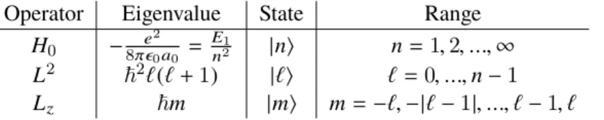
2.1 The figure showsn2β(x)as a function of our radial lattice for a few different cutoffs ink and m (2D) or k andl (3D), demonstrating where we can cut off our sums. The left figure is
for βωz = βωtr/2, where we see we can cut off our sums at very small values. The right
figure is for βωz = βωtr, which represents a phase transition in our system. We can see
these effects in the cutoffs, as shown by the figure on the right, where in2D,n2β(x)fails to converge as we raise the cutoff inkandm. . . 18
2.2 The difference in the second virial coefficient, δb2 = b2(ωz > 0)− b2(ωz = 0) (left) as
a function of rotation frequency βωz in 2D. Noninteracting bn normalized by their
non-rotating, noninteracting values bn(βωz = 0) (right), as functions of n for a few values of βωz and fixed βωtr =5. The ratiobn/bn(βωz =0)is the same in 2D and 3D. . . 22
2.3 Noninteracting Lz/Q1 to third order in the virial expansion in 2D (left) and 3D (right), as
functions of βωz for a few values of βωtr. . . 23
2.4 Noninteracting Iz/Q1 to third order in the virial expansion in 2D (left) and 3D (right), as
functions of βωz for a few values of βωtr. . . 24
2.5 Change in the virial coefficientb2due to the combination of rotation and interaction, for two
(left) and three (right) spatial dimensions. . . 24 2.6 Change in the virial coefficientb3due to the combination of rotation and interaction, for two
(left) and three (right) spatial dimensions. . . 25 2.7 Change in the angular momentum hLˆzi due to the combination of rotation and repulsive
contact interaction, for two (left) and three (right) spatial dimensions, atz =e−2.0. . . 26
2.8 Change in the moment of inertiahIˆzidue to the combination of rotation and repulsive contact
interaction, for two (left) and three (right) spatial dimensions, atz=e−2.0. . . 26
3.1 The Langevin method with real-valued fields versus complex-valued fields. . . 38 3.2 Real (blue) and imaginary (red) density generated by Complex Langevin for a relativistic
Bose gas at finite chemical potential. . . 39 4.1 Thermalization of the Langevin simulation for chemical potentials below the critical point
(left) and above it (right). After thermalization, the running average remains stable despite fluctuations in the individual samples. . . 49 4.2 The real imaginary components of the density as a function of chemical potential, both exact
and CL results, forNx = Nt =4(left) and6(right). . . 52
4.3 Comparison of our results for the density of the relativistic Bose gas at finite potential, against the results of Ref. [1] forNx = Nt =4(left) and6(right). . . 53
4.4 Comparison of our results for the field modulus squared of the relativistic Bose gas at finite potential, against the results of Ref. [1] forNx = Nt =4(left) and6(right). . . 53
5.1 Averages of the observables are taken after discounting some fraction of the evolution, starting attL =0. This gives the system time to thermalize and ensures that our observables
5.2 The field modulus squared (left) and density (right) of the free Bose gas in2+1dimensions via CL, compared with the exact solutions. . . 61 5.3 Density of the superfluid as a function of chemical potential without rotation or interaction and
LIST OF TABLES
1.1 The energyH0, total angular momentumL2, andz-component of the angular momentumLz
LIST OF ABBREVIATIONS
QFT quantum field theory QCD quantum chromodynamics
SCLA semi-classical lattice approximation CL complex Langevin
LIST OF SYMBOLS
G Newton’s gravitational constant e electron charge
0 permittivity of free space ~ reduced Planck constant a0 Bohr radius
S action
Z path integral, grand-canonical partition function vc critical velocity
p energy of excitations of a Bose-Einstein condensate Tc critical temperature
L Lagrangian
λ contact interaction strength
φ complex scalar field ˆ
H Hamiltonian operator
ˆ
T kinetic energy operator
ˆ
V potential energy operator
ˆ
Lz angular momentum operator
ˆ
Iz moment of inertia operator
ˆ
n particle density operator
g bare lattice interaction parameter
β inverse temperature
µ chemical potential
ωtr trapping frequency ωz rotational frequency bn n-th order virial coefficient z fugacity
Ω grand thermodynamic potential
ˆ
P probability
si spin value for lattice sitei J spin interaction coupling H magnetic field strength M magnetization
α spin lattice configuration
K Langevin drift term η Weiner noise term
τ Euclidean time/imaginary time
QN N-body canonical partition function
E energy
Lk|m| associated Laguerre functions Plm(x) associated Legendre functions
a spatial lattice spacing
Nx number of spatial lattice sites
dτ temporal lattice spacing
Nτ number of temporal lattice sites
tL Langevin time Langevin stepsize
V spacetime lattice volume τA autocorrelation time σ2 variance
∆A autocorrelation error
δab kronecker delta
CHAPTER 1: Introduction
Quantum many-body systems are foundational to a wide range of interesting physical topics, from very small scales (the quark-gluon plasma of the early universe) to very large ones (understanding the structure of neutron stars). Advances in theoretical treatment of these systems can aid in the development of novel materials, provide insights into the stability of nuclei, push forward the boundaries of knowledge about the origin of the universe, and more. However, all but the simplest of these systems can be extremely challenging to understand at a detailed level. Very few are accessible using analytical methods, and those which must be calculated computationally frequently have limitations that prevent us from exploring some of the most interesting physics.
This thesis explores one such system: rotating, interacting bosonic systems. The physics at the heart of these systems is relevant across disciplines, from astrophysics to quantum materials to nuclear structure. We begin with the kind of straightforward problem an undergraduate can solve and show how quickly the complexity grows once we consider interacting quantum systems with many particles.
Section 1.1: From two- to many-body systems
1.1.1: The classical N-body problem
As with all complicated problems, it is best to start with the simplest possible version and build from there. To understand the challenges of the quantum N-body problem, we begin with a problem that all
undergraduates learn to solve in the early years of their physics courses: the classical two-body problem1.
The classical two-body problem is most often introduced when students learn orbital mechanics, in the context of the earth-sun interaction. The earth and the sun are two massive objects which exert equal and opposite force on each other. The motion of the two bodies is determined by the gravitational force between them. Since this force is a Newton’s third law pair, we are able to take advantage of the symmetries and conservation laws of this system to greatly reduce the complexity of the problem.
The total momentum of the system is a conserved quantity, so we can perform a change of variables. Instead of measuring our coordinatesr1 andr2 relative to some external origin, we choose to express the
equations above in terms of the center of mass coordinate measured relative to that external origin,R, and the relative separation between the two bodies,r, and then the principles of conservation of momentum can be applied. Since the total momentum is conserved, the center of mass velocity must be constant, and therefore the center of mass motion, denoted byR, becomes a simple linear function of time:
R=vCMt (1.1)
and our two-coordinate problem has now been reduced to a one-coordinate problem. All that remains is to solve forrwhich, while often not trivial, is something that can be done in a straightforward manner.
This classical two-body problem serves as a starting point for the more complicated classical N-body
problem, which can’t be solved by hand for largeN, but can be solved numerically. The equations of motion
are given by
¨ri =−G N
X
j=1,j,i
mj(ri−rj)
|ri−rj|3
. (1.2)
This is a6N-dimensional ordinary differential equation with time being the only degree of freedom and can
be solved for some large number of objects,N, with memory requirements scaling linearly with the number
of objects.
This is, as mentioned above, a much simpler case than the quantum N-body problem, but it serves to
establish the approaches to problems such as these: use symmetries and conservation laws to reduce the problem complexity and then solve computationally. Unfortunately, as we shall soon see, this is a necessary but not sufficient step for studying quantum many-body systems, and quantum many-body problems will require more sophisticated methods to solve, even computationally.
1.1.2: The quantum N-body problem
mechanics we solve the Schrödinger equation. The Schrödinger equation for the hydrogen atom is:
−
~2∇2p
2mp + ~2∇2e
2me + e2
4π0r
Ψ(re,rp) =EΨ(re,rp), (1.3)
whereris here defined as the magnitude of the separation between the electron and the proton,r = |re−rp|[4–
6],Eis the energy of the system, and we are solving for the quantum wave-function,Ψ.
This equation has two useful features which make it a relatively simple problem. First, the solutions to this equation have no time dependence; and second, since the Coloumb potentialV(r) = −4πe2
0r depends
only on the separationr =|re−rp|, a change of variables can be applied, and the equation can be separated
into two independent equations, just as we did in the classical two-body problem, where our central potential was gravitational rather than electrical.
The appropriate change of variables is fromreandrpto the center of mass coordinateRand the relative
coordinater, defined below:
R= mere+mprp
me+mp , and
r=re−rp. (1.4)
With the introduction of total (M= me+mp) and reduced (µ= memp
M ) masses, the new Schrödinger equation
is given by:
"
− ~
2
2M∇ 2 R−
~2
2µ∇
2 r −
e2
4π0r
#
Ψ(R,r) =EΨ(R,r), (1.5)
which can be solved using separation of variables.
The solution to the center of mass equation is that of a free particle of mass M (just as in the classical case), making it uninteresting to the internal structure of the hydrogen atom. It is the solution to the relative motion equation which is of interest; the relationship between the proton and electron is what gives the hydrogen atom its quantized values of energy and angular momentum.
This is an eigenvalue problem, and the solutions toΨ(r, θ, φ) =Ylm(θ, φ)R(r)are the joint eigenstates
of the energy (Hˆ) and angular momentum operators (Lˆ2andˆL
z). For simplicity, we define a dimensionless
coordinate, ρ= r
a0, where
The constanta0is the Bohr radius, which is a physical constant corresponding to the average distance of the
electron from the nucleus in the ground state. Now the radial equation reads:
−d dρ ρ2
dR(ρ)
dρ
!
+
`(`+1)−2ρ−EHρ2
R(ρ) =0 (1.7)
The solutions to this equation are related to the associated Laguerre polynomialsLkn[7]:
Rn`(r)= N
2r na0
!`
e−r/(na0)Ln2`++`1 2r na0
!
, (1.8)
where ` and n are integers and N is obtained by normalizing the radial wave function. Thus, the final
hydrogen wave functions are described by
Ψ(r)= N 2r
na0
!`
e
−r
n a0L2`+1
n+`
2r na0
!
Y`m(θ, φ) (1.9)
withn, `,andmall quantum numbers describing the state. The unperturbed hydrogen energy eigenstates are
Operator Eigenvalue State Range
H0 − e
2
8π0a0 =
E1
n2 |ni n=1,2, ...,∞
L2 ~2`(`+1) |`i `=0, ...,n−1
Lz ~m |mi m=−`,−|`−1|, ..., `−1, `
Table 1.1: The energyH0, total angular momentumL2, andz-component of the angular momentumLzare all operators which are
simultaneous eigenstates of the unperturbed hydrogen Hamiltonian.
eigenstates of three operators simultaneously: the Hamiltonian or bare hydrogen atom energyHˆ (principal quantum number, n), the total angular momentum squared ˆL2 (angular quantum number `), and the z
-component of angular momentumˆLz (magnetic quantum numberm). Table 1.1 illustrates these values, the operators they correspond to, their eigenvalues and eigenvectors (states), and the restrictions on their range. Beyond the hydrogen atom, we quickly depart the realm of exactly-solvable quantum systems. While in principle, the process is straightforward (i.e. solve the N-body Schrödinger equation), in practice, this
is only possible for a small number of scenarios, often ones which tell us very little about the complicated physics seen in the universe. The presence of more than two particles with at least a two-body interaction quickly yields intractable equations.
star? – are about large numbers of particles interacting with each other and the environment, this provides a strong motivation for developing new methods to solve for the equations of motion of these systems. Many approaches have been taken to this challenge, and different disciplines prefer different classes of methods. Mean-field theories and related approaches are common in condensed matter and materials science; coupled cluster approaches are often seen both in nuclear theory and quantum chemistry; and lattice gauge theory is employed largely in relativistic systems like quantum chromodynamics (QCD) and quantum electrodynamics (QED). These methods are all united by the need for computational resources to evaluate these numerically-intensive systems.
Section 1.2: Stochastic methods and the sign problem
Computational methods have allowed for great advances in understanding of quantum many-body sys-tems. However, limitations still exist. The computational complexity of many quantum problems scales exponentially with the size of the system due to the size of the underlying Hilbert space, meaning that many systems of great interest are still inaccessible due to lack of fast or powerful enough computers. Nuclear structure is one such example; numerical solutions to the many-nucleon Schrödinger equation can only be achieved for nuclei with atomic mass number of up to four. With well-controlled approximations and innovative methods, calculations can be done for heavier nuclei – up to nickel (A= O(60)) [8]. Innovative methods are what drive advancement in many-body quantum mechanics. Exact solutions to the many-body Schrödinger equation simply require more computational resources than exist, and so creative and intelligent alternatives must be developed.
Among these alternatives are quantum Monte Carlo (QMC) methods. These are a well-established set of methods for calculating properties of quantum many-body systems. Their applications cover a massive range of energy scales, from QCD toab initionuclear structure to neutron stars, and they provide a stable
technique for calculating properties of these systems. These methods take advantage of similarities between path integral formulations of quantum mechanics and the statistical mechanics partition function in order to construct a well-behaved probability distribution from which behavior of the system can be sampled using a Markov chain method.
the action. This allows for the calculation of observables, as shown here:
Z =
Z
DxeiS[x] (1.10)
hOi = 1
Z
Z
DxeiS[x]O(x). (1.11)
Assuming a real action,S[x], the complex weight can be made real by performing a Wick rotationit → τ, such that now our observable is the integral of that observable over all paths x weighted by a probability
measure for that path:
hOi = 1
Z
Z
DxP(x)O(x). (1.12)
P(x) = e−S[x]. (1.13)
This formulation lends itself to a stochastic treatment of the path integral.
Quantum many-body problems can be written in terms of quantum fields, using quantum field theory (QFT). The fields can then be discretized and placed on a spacetime lattice, a strategy known as lattice field theory. The benefit of lattice methods is that the resulting path integral can often be evaluated stochastically, and the expectation value of an observable can be given by
hOi ≈ 1
N N
X
n=1
On, (1.14)
where N is the number of configurations sampled, and On is the value of the observable calculated with
lattice configurationn. If a good probability measure can be defined for the system, i.e. ifP(x) = e−S[x]
is real and positive-definite, then the solution is exact with systematic uncertainties determined entirely by lattice parameters and statistical uncertainties due to the number of samples. Thus, overall uncertainty can be controlled by varying lattice size and spacing and number of samples.
1.2.1: The sign problem in quantum many-body physics
this case, the crucial step for QMC approaches – i.e. treating the weight like a probability distribution from which we can sample values of the fields and the observables – becomes invalid.
If the action of a quantum many-body system is real and positive, we can use standard Monte Carlo methods to evaluate the path integrals and compute observables. Howevever, there are many very important cases when this condition is not satisfied, for example strongly-interacting QCD systems with non-vanishing chemical potential and superconductors and superfluids under specific conditions. The sign problem con-founds our ability to make progress in these areas with the methods that have been so effective in so many quantum many-body systems. In order to move forward in understanding these systems, we must develop new methods to circumvent the sign problem.
Section 1.3: Superfluidity
Superfluids, in the simplest terms, are fluids that flow without friction. In slightly less simple terms, they transport a conserved charge (e.g. mass, particle number, electric charge) without loss of energy due to dissipation for velocities smaller than some critical velocity:
vc=min p
p
p (1.15)
wherepis the energy of the excitations on the condensate andpis its corresponding momentum.2
This behavior was first observed in liquid helium, but can appear in a wide range of substances. Su-perfluidity is in fact a phase of a system, which occurs below a critical temperature. This temperature can vary wildly across systems, which means superfluidity is a state observed across a dramatic range of energy scales, from helium and other ultracold atomic gases at one end (Tc ≈ 10−7K) to quark matter at the other
end (Tc ≈1011K).
The frictionless flow of a superfluid is not its only remarkable behavior. Superfluid velocity has no curl, and therefore is irrotational. However, nonzero hydrodynamic circulation can exist, and must be quantized in units of 2π~/m, where m is the mass of the particles comprising the superfluid. If we try to rotate
superfluid helium – or another cold atomic gas – it develops spontaneous vortices in direct proportion to the amount of angular momentum imposed on the system. This has been predicted as a direct result of the properties of superfluids (see e.g. Refs. [11–13]) and observed in experiments with ultracold atoms (see e.g.
Refs [14–17]).
Superfluids share much with their phenomenological cousin, superconductors. While the two phenomena are not identical, superconductors are also a phase of a system in which a conserved charge is transported without energy loss. Superconductors break a local symmetry, while superfluids break a global symmetry – this is the fundamental difference that separates them on a theoretical level. The strong connections between the two – particularly their dissipationless transport – makes them together a subject of active inquiry.
We can build a theory of superfluids using a complex scalar field. The Lagrangian of the system will be invariant under U(1) symmetry, and a necessary condition for superfluidity is the spontaneous breaking of this U(1) symmetry, i.e. the ground state of the system will not be invariant under this symmetry even though its Lagrangian is. The critical temperature is the point above which the superfluid has “melted," i.e. the point where the ground stateissymmetric under U(1).
Our system – which can become a superfluid below some critical temperature – is a complex scalar field, representing spin-0bosons with massmand interacting via a repulsive contact interactionλ >0. The
Lagrangian for our system is as follows
L =∂µφ∗∂µφ−m2|φ|2−λ|φ|4 (1.16)
This Lagrangian is invariant under U(1) rotations of the field, that isL is unchanged for
φ→e−iαφ (1.17)
which is a global symmetry, asαis a constant and does not depend on spacetime.
There will also be a conserved charge – this is what is transported by the superfluid without loss of energy – and this will arise from Noether’s theorem. Generally, the conserved charge of interest with superfluids is a particle number charge.
like superfluidity, with a vanishing resistivity below some critical temperature.
Helium 3 is also fermionic, but forms Cooper pairs due to an attractive interaction between the atoms, and can form multiple different superfluid phases. This has been observed in other ultracold atomic gases, most notably by the Ketterle group [18], where vortex formation in lithium 6 demonstrated a superfluid state. In high-energy physics, color superconductors may form in quark matter and inside dense stars.
Section 1.4: Superfluids and rotation
The spontaneous appearance of quantized vortices in a lattice structure is a characteristic feature of superfluids at thermal equilibrium [19–22]. These effects are related to rotation and also external magnetic fields [23], and the vortices can have dynamics that interact with sound waves [24]. Addition of spin-orbit coupling creates further complexity in the system, leading to unique phases depending on the type of coupling [25–28]
In 1949, Lars Onsager first predicted that vortices would form in rotating superfluids [12]. Richard Feynman expanded on Onsager’s prediction a few years later, reiterating the expectation that quantized vortices would appear when superfluids were forced to rotate [13]. Another thirty years after these predictions, the first direct observation of quantum vortices was made in rotating superfluid4He [29]. Experimentally,
great progress has been made in studying rotating superfluids since the first direct observation of vortex formation. In 2000, vortex formation was observed in stirred, magnetically-trapped rubidium atoms [17]. The next year, triangular vortex lattices of up to 130 vortices were observed in rotating ultracold sodium atoms [14]. Ultracold atoms provide a highly controlled, tuneable setting for studying vortex formation and other properties of rotating superfluids.
Adding rotation into a complex scalar field introduces new challenges into theoretical treatments of the system. While a nonrelativistic complex scalar field already yields a potential sign problem in stochastic treatments, there are ways to get around this sign problem. The additional complexity of the angular momentum term in the action eliminates those possibilities and yields an irretrievably complex weight for stochastic sampling. As a result, most theoretical work done on rotating superfluids is done using mean-field treatments such as the Gross-Pitaevskii Equations (GPE). These equations have been very successful in describing mean-field behavior of rotation in superfluids, including the spontaneous formation of vortices, but stop short of a fully quantum examination of the system [19].
condensed matter for understanding the effect of a magnetic field on superconductors, in nuclear physics for describing the behavior of rotating nuclei, and in astrophysics for illuminating the physics of neutron stars and pulsars. In order to continue to progress in these areas of physics, a method to work around the sign problem must be used. Theoretically, treatment of these systems has stalled due to the presence of the sign problem, and the subject of this thesis is to explore alternative methods to understanding rotating bosonic systems.
Section 1.5: Outline
CHAPTER 2: Semi-classical lattice approximation for trapped, rotating, interacting quantum matter
Section 2.1: Motivation: why use a semi-classical lattice approximation?
One way to avoid the sign problem quantum many-body systems is to use approximate methods. Despite their limitations, approximations are excellent tools that can allow us to examine interesting behavior in particular regimes without having to encounter the sign problem that can arise in a full stochastic calculation. Often, they are our only way to benchmark numerical results.
In this case, we apply the virial expansion to a system of trapped, rotating, interacting bosons in 2D and 3D and implement a semiclassical lattice approximation (SCLA) recently put forward in Refs. [30–32], where it was applied to non-rotating matter.While these systems are not in themselves rotating superfluids, they have the same field theoretical structure and in the right temperature and density regime could support superfluidity. The approximation allows us to bypass the requirement of solving the N-body problem
to access the n-th order virial coefficient and describe the thermodynamics of the system using a virial
expansion. The virial expansion is valid in a high-temperature, low-density limit, while the semi-classical lattice approximation requires that we use a strongly-interacting or weakly-interacting regime. In this case, we look at the weakly-interacting case, where the interaction potential is significantly smaller than the noninteracting Hamiltonian.
Section 2.2: Hamiltonian and formalism
We use a Hamiltonian formalism to generate our virial coefficients, as it lends itself well to the manip-ulation of the partition function. Our Hamiltonian is composed of both a non-interacting term H0 and an
interacting termHint:
ˆ
H= Hˆ0+Vˆint. (2.1)
The noninteracting term can be further broken up into three contributions:
ˆ
where
ˆ
T= X
s=1,2
Z
ddxψˆs†(x) −~
2∇2
2m
!
ˆ
ψs(x), (2.3)
is the kinetic energy,
ˆ
Vext=1
2mω
2
tr
Z
ddxx2(nˆ1(x)+nˆ2(x)), (2.4)
is the spherically symmetric external trapping potential inddimensions, and
ˆ
Lz=i
X
s=1,2
Z
ddxψˆs†(x)x∂y−y∂x
ˆ
ψs(x), (2.5)
is the angular momentum operator in thezdirection. The interaction term is given by
ˆ
Vint=−g
Z
ddxˆn1(x)ˆn2(x), (2.6)
with g the bare interaction parameter, and where, for the sake of simplicity, we restrict ourselves to two particle species with a contact interaction across species (i.e. no intra-species interaction).
In the above equations, the field operatorsψˆs,ψˆ†
scorrespond to particles of speciess =1,2, andnˆs(x)are
the coordinate-space densities. In the remainder of this chapter, we will use units such that~= kB=m=1.
2.2.1: Thermodynamics and the virial expansion
The grand-canonical partition function describes the statistical properties of the the quantum many-body system, as all the thermodynamic quantities of interest can be determined from it. It has the general form
Z=Tre−β(Hˆ−µNˆ)
=e−βΩ, (2.7)
where βis the inverse temperature,Hˆis the Hamiltonian given in Eq. (2.1),Ωis the grand thermodynamic
potential,Nˆis the total particle number operator, andµis the overall chemical potential.
is given by
−βΩ=lnZ =Q1
∞
X
n=1
bnzn. (2.8)
The coefficients bn are known as the virial coefficients, andQ1 is the one-body partition function, which
can be calculated directly without too much trouble, as there is no interaction present (we will show this calculation in Section. 2.2.2). This expansion is valid for small values of the fugacity, which can be affected by both the temperature (T ∝1/ β) and chemical potential of the system.
We can compare this virial expansion for the partition function with the expression of the grand-canonical partition function in terms of the canonical partition functionsQN of all possible particle numberN:
Z=
∞
X
N=0
zNQN, (2.9)
and thereby obtain expressions for the virial coefficients
b1 = 1, (2.10)
b2 = Q2 Q1
− Q1
2!, (2.11)
b3 = Q3 Q1
−b2Q1− Q
2 1
3!, (2.12)
and to higher order. The quantity we are interested in is the change in these virial coefficients due to rotation:
δbn=b(n0)(|ωz| >0)−b(n0)(ωz =0) (2.13)
and due to the presence of interactions:
∆bn= bn−b(n0) (2.14)
whereb(n0)is the virial coefficient of the system when there are no interactions.
bparticles of type 2:
Q1 = Q1,0+Q0,1 =2Q1,0, (2.15)
Q2 = Q2,0+Q0,2+Q1,1 =2Q2,0+Q1,1, (2.16)
Q3 = Q3,0+Q0,3+Q2,1+Q1,2 =2Q3,0+2Q2,1, (2.17)
and so on for higher orders. In the absence of intra-species interactions, only theQ1,1andQ2,1are affected,
such that the change inb2andb3due to interactions is entirely given by
∆b2 =
∆Q1,1
Q1
, (2.18)
∆b3 =
2∆Q2,1 Q1
−∆b2Q1. (2.19)
We will use these expressions to access the high-temperature thermodynamics of the bosons in this system and examine their dependence on the rotation frequency (expressed in dimensionless form as βωz), the strength
of the trapping potential (in dimensionless form, βωtr), and inter-particle interaction (whose dimensionless
form,λ, will depend on the bare couplinggand the dimensionalityd).
2.2.2: Semiclassical lattice approximation
To calculate the interaction-induced change in the canonical partition functions∆Q1,1and∆Q2,1, we use
an approximation. The exponential of the sum of two non-commuting operators can be related to the product of the two exponentiated operators via an infinite series (the Baker-Campbell-Hausdorff formula) [6, 33]:
eA+B =
∞
X
n=0
(A+B)n
n! = I+ A+B+ 1
2(A+B)(A+B)+. . . (2.20)
eAeB = eA+B+12[A,B]+... (2.21)
Our approximation consists in keeping only the leading term in the Magnus expansion derived from the Baker-Campbell-Hasudorff formula:
e−β(Hˆ0+Vˆint) =e−βHˆ0e−βVˆint×e−β 2
2 [ ˆH0,Vˆint]×. . . , (2.22)
can be ignored (i.e. respectively the strong- and weak-coupling limits).
Single-particle bases in 2D and 3D
In evaluating the results of the semiclassical lattice approximation, we will make use of the eigenstates ofHˆ0in 2D polar coordinates and 3D spherical coordinates.
Two spatial dimensions.- The single-particle eigenstates ofHˆ0in 2D are given by
hx|ki= √1
2πRkm(ρ)e
imφ, (2.23)
where
Rkm(ρ)= Nkm(2D)
√
ωe−ρ2/2
ρ|m|
Lk|m|(ρ2), (2.24)
where ρ=√ωr and
Nkm(2D) =
√ 2
s
k!
(k+|m|)!, (2.25)
withLk|m| the associated Laguerre functions. We have used polar coordinatesr, φ, and a collective quantum
numberk= (k,m), withk =0,1, . . . andmany integer value. The corresponding energy is
Ekm=ωtr(2k+|m|+1)+ωzm (2.26)
These eigenstates are derived in more detail in Appendix A.1.
Three spatial dimensions.- The single-particle eigenstates ofHˆ0in 3D are
hx|ki= Rkl(ρ)Plm(cosθ)eimφ, (2.27)
wherePlm(x)are the associated Legendre functions and
Rkl(ρ)= Nkl(3D)ω3tr/4e−ρ
2/2
ρlLl+1/2 k (ρ
where
Nkl(3D) =
s
1 √
4π
2k+2l+3k!
(2k+2l+1)!!. (2.29)
Here, we have used spherical coordinatesr, θ, φ, whereθis the polar angle, andφthe azimuthal angle. The collective quantum numberk = (k,l,m) is such thatk ≥ 0,l ≥ 0, and−l ≤ m ≤ l. The corresponding
energy is
Ek`m=ωtr(2k+l+3/2)+ωzm. (2.30)
The eigenstates in 3D have been derived in great detail in many references, as the single-particle wave function is the same as that of an electron in a hydrogen atom. For detailed derivations, see e.g. Refs [4–7].
Single-particle partition functionQ1
As mentioned above, Q1 can be computed straightforwardly. The single-particle partition function is
described as
Q1 =
X
k
e−βEk. (2.31)
Thus, in 2D,
Q1 =2
X
k,m
e−βEk m = 2e
−βωtr
(1−e−βω+)(1−e−βω−), (2.32)
whereω±=ωtr±ωz and the overall factor of 2 reflects the fact that we have two particle species.
Similarly, in 3D,
Q1 =2e−βωtr3/2
1
(1−e−2βωtr)(1−e−βωz) "
1 1−e−βω− −
e−βωz
1−e−βω+
#
Two-body contribution∆Q1,1.
The calculation of the first nontrivial virial coefficient,∆b2, in our semiclassical approximation requires
the above result forQ1and∆Q1,1. At leading order,
Q1,1=Tr1,1
e−βHˆ0e−βVˆint
, (2.34)
whereTr1,1 represents the trace of the matrix when we have a single particle of each species. This leads to
Q1,1 =
X
k1,k2,x1,x2
hk1k2|e−β ˆ H0|x
1x2ihx1x2|e−β ˆ Vint|k
1k2i
= X
k1,k2,x1,x2
e−β(Ek1+Ek2)Mx
1,x2|hk1k2|x1x2i|
2, (2.35)
where we have inserted complete sets of states in coordinate space {|x1x2i} and in the basis |k1k2i of
eigenstates ofHˆ0, whose single-particle eigenstates|kihave eigenvaluesEk. We have also made use of the fact thatVˆintis diagonal in coordinate space, such that
Mx1,x2 =1+Ba
−dδ
x1,x2, (2.36)
whereB=ad eβgd D −1and we have introduced a spatial lattice spacingaas a regulator. This leads to a
new expression for∆Q1,1:
∆Q1,1 =B
X
k1,k2,x
ade−β(Ek1+Ek2)|hk
1k2|x xi|2, (2.37)
which can be computed numerically.
The computationally demanding part of this calculation is the overlap function |hk1k2|x xi|2. Note that
this function can be factorized as|hk1|xi|2|hk2|xi|2. Upon summing overk1, however we obtain a simpler
expression
∆Q1,1 =B
X
x
where
nβ(x) =X k
e−βEk|hk|xi|2. (2.39)
The exponential decay with the energy will enable us to cut off the sum over k in most cases without significantly losing precision. We show a representative example of such cutoff effects in Figure 2.1. We can see in this figure that the relationship between the rotation frequency and trapping potential has an effect on where we can cut off our sum. We see that in 2D whenωz =ωtr, our sum does not converge as we raise
the cutoff limit fork andm, but instead grows with that cutoff. This same effect is not visible for values of ωz < ωtr.
This shows that at the specific point where ωz = ωtr, we can no longer calculate virial coefficients
efficiently in 2D. Fortunately, we are not concerned with the system at phase transition, but instead we are interested in what happens below the critical rotation frequency.
0.0 0.5 1.0 1.5 2.0 2.5 3.0 3.5 4.0
0.0 0.1 0.2 0.3 0.4 0.5 0.6 0.7
n
2()/ d tr
2D, k = 2, m = 1 2D, k = 4, m = 2 2D, k = 8, m = 4 2D, k = 16, m = 8 3D, k = 2, l = 2 3D, k = 4, l = 4 3D, k = 8, l = 8 3D, k = 16, l = 16
0.0 0.5 1.0 1.5 2.0 2.5 3.0 3.5 4.0
0.0 0.1 0.2 0.3 0.4 0.5 0.6 0.7
n
2()/ d tr
2D, k = 2, m = 1 2D, k = 4, m = 2 2D, k = 8, m = 4 2D, k = 16, m = 8 3D, k = 2, l = 2 3D, k = 4, l = 4 3D, k = 8, l = 8 3D, k = 16, l = 16
Figure 2.1: The figure showsn2β(x)as a function of our radial lattice for a few different cutoffs inkandm(2D) orkandl(3D),
demonstrating where we can cut off our sums. The left figure is for βωz =βωtr/2, where we see we can cut off our sums at very
small values. The right figure is forβωz=βωtr, which represents a phase transition in our system. We can see these effects in the
cutoffs, as shown by the figure on the right, where in2D,n2β(x)fails to converge as we raise the cutoff inkandm.
To compute the sum, we refer back to the previously-defined single-particle eigenstates in 2D (Eq. (2.23)), arriving at an expression in 2D fornβ:
nβ(x) =ωtre −ρ2
2π
X
k,m
e−βEk mf2D
km(ρ
2), (2.40)
of the radial coordinate (concentric with the trapping potential). Here,
fkm2D(ρ2)≡ 2k! (k+|m|)!ρ
2|m|
Lk|m|(ρ2)2, (2.41)
Similarly, in 3D,
nβ(x) =ω3tr/2e −ρ2
√ 4π
X
k,l,m
e−βEk l mf3D
kl (ρ 2)(Pm
l (cosθ))
2 (2.42)
where
fkl3D(ρ2) ≡ 2
k+2l+3k!
(2k+2l+1)!!ρ
2l
Llk+1/2(ρ2)2 (2.43)
Which can be used to calculate∆Q1,1using Eq. (2.38).
Calculation of∆Q2,1
Following the same steps outlined above, it is straightforward to show that
∆Q2,1 =
B
2
X
k1k2k3
e−β(Ek1+Ek2+Ek3) X
x1x2
|hx1x2x1|k1k2k3i|2. (2.44)
The overlap can be simplified slightly by factoring across distinguishable species:
hx1x2x1|k1k2k3i = hx1x2|k1k2ihx1|k3i, (2.45)
where the matrix elementhx1x2|k1k2iis a permanent of single-particle states:
hx1x2|k1k2i=hx1|k1ihx2|k2i+hx2|k1ihx1|k2i. (2.46)
As in the case of∆Q1,1, we will sum over the energy eigenstates first, and then perform the spatial sum.
To that end, it is useful to define
nBβ(x1,x2)=
X
k1k2
e−β(Ek1+Ek2)|hx
such that,
∆Q2,1 =
B
2
X
x1x2
nβB(x1,x2). (2.48)
As in the case of nβ(x), the exponential decay with the energy allows us to cut off the double sum in
nBβ(x1,x2)without significantly affecting the precision of the whole calculation.
2.2.3: Gauss-Hermite quadrature
As shown above, the single-particle wavefunctions (Eq. (2.23) and Eq. (2.27)) and the associated density functionsnβ(x)andnβB(x1,x2) are governed in the radial variable by a Gaussian decay. For that reason, it
is appropriate to calculate the corresponding integrals using Gauss-Hermite quadrature. The corresponding
MpointsxiandMweightswiallow us to estimate integrals according to
Z ∞
−∞
dx e−x2f(x)=
M−1
X
i=0
wif(xi). (2.49)
In this work we use the same quadrature points and weights as in our previous work of Refs [34–36]. Section 2.3: Results
2.3.1: Noninteracting virial coefficients at finite angular momentum
We present here the calculation of the noninteracting (i.e. g = 0) virial expansion whenωz , 0. We
begin with the partition function of spin-1/2bosons in terms of the single-particle energiesE:
lnZ =2X
E
ln(1−ze−βE). (2.50)
This can be further expanded for smallz(the virial expansion) as
lnZ =−2X
E
∞
X
n=1 zn
n e
−nβE. (2.51)
Two spatial dimensions.- In 2D,E = Ekm = ωtr(2k+|m|+1)+ωzm, wherek ≥ 0andmis summed
over all integers. Thus, we may write the sum as
lnZ =−2X
E
∞
X
n=1
zne−nβωtr
n
X
k
e−βωtr2nk
∞
X
m=0
e−nmβω++
∞
X
¯ m=1
e−nm¯βω−
whereω±=ωtr±ωz. Carrying out the sums overk,m,m¯, we obtain
lnZ =Q1
∞
X
n=1
bnzn, (2.53)
where
Q1bn=
−2
n
e−nβωtr
(1−e−nβω+)(1−e−nβω−). (2.54)
Finally, to determinebnwe useQ1as derived above in Eq. (2.32)), such that
bn=
−1
n e
−βωtr(n−1) (1−e−βω+)(1−e−βω−)
(1−e−nβω+)(1−e−nβω−). (2.55)
Note that, while thebnare always finite,Q1diverges whenω−→0. This signals an instability due to the fact that, for anyω−<0, i.e. ωz > ωtr, the system does not have a ground state. In terms oflnZ, the divergence may be regarded as a phase transition atωz =ωtr. In other words, in that limit the centrifugal motion due to the rotation is strong enough to overcome the trapping potential and the system escapes to infinity.
Three spatial dimensions.- In 3D, E = Eklm = ωtr(2k +l+3/2)+ωzm, where k ≥ 0, l ≥ 0, and
−l ≤ m≤l. Therefore, analyzing the problem as in the 2D case, we obtain
Q1bn=
−2
n
e−32nβωtr
(1−e−nβωtr)(1−e−nβω+)(1−e−nβω−), (2.56)
and using (Eq. (2.33), we determine
bn=
−1
n e
−32βωtr(n−1) (1−e−βωtr)(1−e−βω+)(1−e−βω−)
(1−e−nβωtr)(1−e−nβω+)(1−e−nβω−). (2.57)
As in the 2D case, thebnare always finite, butQ1diverges whenω−→0.
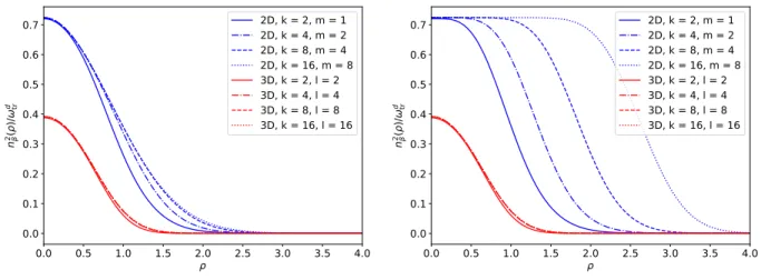
The impact of rotation, i.e. a finite βωz on a noninteracting system is displayed in Figure 2.2. In both
2D and 3D, the angular momentum has an approximately linear dependence on the rotation frequency, with the slope of the line decreasing for larger trapping potentials. In 2D, the trap frequency has a much more pronounced effect than in 3D, with the angular momentum collapsing to nearly a flat line for βωtr >2, while
0 2 4 6 8 10 z
1.0 0.8 0.6 0.4 0.2 0.0
b2
tr= 0.0 tr= 1.0 tr= 2.0 tr= 3.0 tr= 4.0 tr= 5.0
1.0 1.5 2.0 2.5 3.0 3.5 4.0 4.5 5.0
n
0.65 0.70 0.75 0.80 0.85 0.90 0.95 1.00
bn /bn
(
z
=
0)
z= 0.0 z= 1.0 z= 2.0 z= 3.0 z= 4.0 z= 5.0
Figure 2.2: The difference in the second virial coefficient,δb2=b2(ωz>0)−b2(ωz=0)(left) as a function of rotation frequency
βωzin 2D. Noninteractingbnnormalized by their non-rotating, noninteracting valuesbn(βωz=0)(right), as functions ofnfor a
few values ofβωzand fixedβωtr=5. The ratiobn/bn(βωz=0)is the same in 2D and 3D.
2.3.2: Noninteracting thermodynamics at finite angular momentum
We can now derive a virial expansion for the angular momentumLz and thezcomponent of the moment
of inertiaIz:
hˆLzi=− ∂lnZ
∂(βωz) = Q1
∞
X
n=1
Lnzn, (2.58)
where
Ln=nbn
e−nβω+−e−nβω−
(1−e−nβω+)(1−e−nβω−), (2.59)
and
hˆIzi=−
∂2lnZ ∂(βωz)2
=Q1
∞
X
n=1
Inzn, (2.60)
where
In=
1
Q1
∂(Q1Ln)
∂(βωz) =−nLn
"
e−nβω++e−nβω−
e−nβω+−e−nβω− +
2(e−nβω+−e−nβω−)
(1−e−nβω+)(1−e−nβω−) #
. (2.61)
to a system beyond the scope of our study.
Remarkably, because the dependence ofQ1bnonω+andω−is the same in 2D and 3D, the relationship betweenLnandbnis identical in 2D and 3D. It follows that the relationship betweenInandbnis identical
in 2D and 3D as well. Thus, any differences in the angular momentum and moment of inertia between two and three dimensions arises entirely from the differences between the virial coefficientsbn.
Furthermore, atωz =0, a finite moment of inertia remains, in 2D:
In→2n(−1)ne−(2n−1)βωtr
(1−e−βωtr)2
(1−e−nβωtr)4, (2.62)
and in 3D:
In→2n(−1)ne−
1
2βωtr(5n−3) (1−e
−βωtr)3
(1−e−nβωtr)5. (2.63)
which characterizes the static response to small rotation frequencies within the virial expansion, as a function of βωtr.
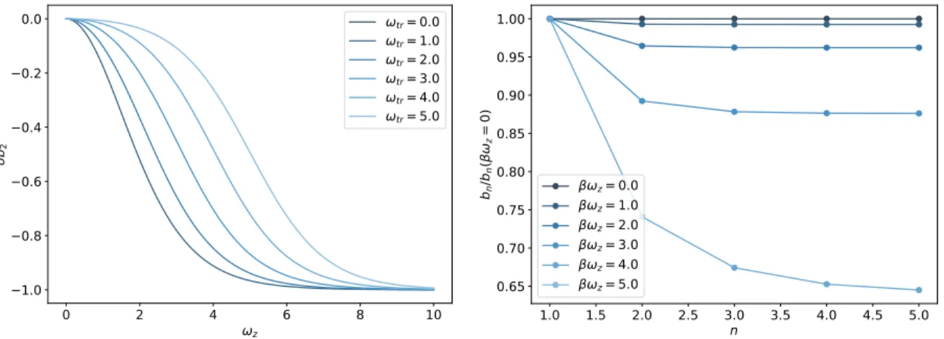
The impact of rotation on the angular momentum for a noninteracting system is shown in Figure 2.3, and the impact of rotation on the moment of inertia for a noninteracting system is shown in Figure 2.4
0.00 0.05 0.10 0.15 0.20 0.25
z/ tr 0.000
0.005 0.010 0.015 0.020 0.025
Lz /Q1
tr= 1.0 tr= 2.0 tr= 3.0 tr= 4.0 tr= 5.0
0.00 0.05 0.10 0.15 0.20 0.25
z/ tr 0.000
0.025 0.050 0.075 0.100 0.125 0.150 0.175
Lz /Q1
tr= 1.0 tr= 2.0 tr= 3.0 tr= 4.0 tr= 5.0
Figure 2.3: NoninteractingLz/Q1to third order in the virial expansion in 2D (left) and 3D (right), as functions of βωzfor a few
values ofβωtr.
2.3.3: Interacting virial coefficients at finite angular momentum
0.00 0.05 0.10 0.15 0.20 0.25 z/ tr
0.00 0.02 0.04 0.06 0.08 0.10 0.12
Iz /Q1
tr= 1.0 tr= 2.0 tr= 3.0 tr= 4.0 tr= 5.0
0.00 0.05 0.10 0.15 0.20 0.25
z/ tr 0.0
0.2 0.4 0.6 0.8
Iz /Q1
tr= 1.0 tr= 2.0 tr= 3.0 tr= 4.0 tr= 5.0
Figure 2.4: NoninteractingIz/Q1to third order in the virial expansion in 2D (left) and 3D (right), as functions ofβωzfor a few
values ofβωtr.
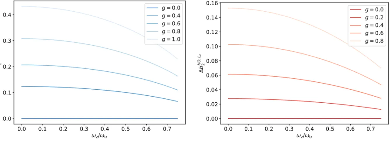
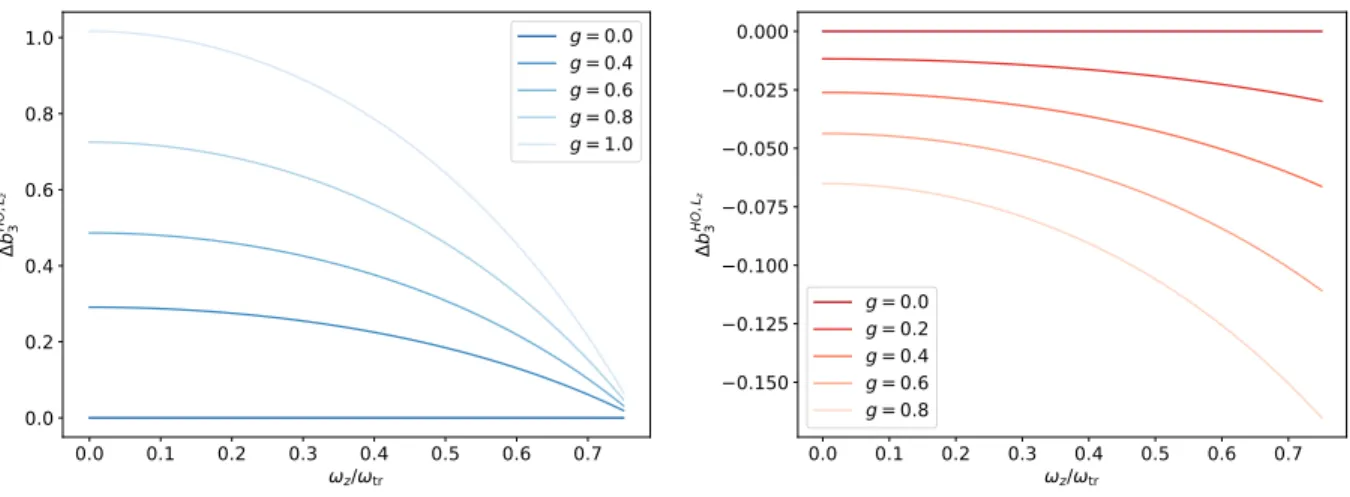
coefficients,b2 andb3 are shown in Figure 2.5 and Figure 2.6 for a range of bare couplings fromg =0to g = 1as a function ofωz/ωtr. In all cases, the magnitude of the change in the virial coefficient increases
as the interaction strength, g, increases, but the behavior varies with increases inωz/ωtr. (Recall that as ωz/ωtr→1, the system undergoes a phase transition.)
0.0 0.1 0.2 0.3 0.4 0.5 0.6 0.7
z/ tr 0.0
0.1 0.2 0.3 0.4
b
HO
,Lz
2
g = 0.0 g = 0.4 g = 0.6 g = 0.8 g = 1.0
0.0 0.1 0.2 0.3 0.4 0.5 0.6 0.7
z/ tr 0.00
0.02 0.04 0.06 0.08 0.10 0.12 0.14 0.16
b
HO
,Lz
2
g = 0.0 g = 0.2 g = 0.4 g = 0.6 g = 0.8
Figure 2.5: Change in the virial coefficientb2due to the combination of rotation and interaction, for two (left) and three (right)
spatial dimensions.
The change in∆b2 is similar in 2D and 3D, although the effect is much larger in 2D. The next virial
coefficient,∆b3, behaves very differently in 2D than it does in 3D. We can see that in 2D,∆b3 looks very
similar to ∆b2, while in 3D,∆b3 is negative rather than positive and its magnitude increases rather than
0.0 0.1 0.2 0.3 0.4 0.5 0.6 0.7 z/ tr
0.0 0.2 0.4 0.6 0.8 1.0
b
HO
,Lz
3
g = 0.0 g = 0.4 g = 0.6 g = 0.8 g = 1.0
0.0 0.1 0.2 0.3 0.4 0.5 0.6 0.7
z/ tr 0.150
0.125 0.100 0.075 0.050 0.025 0.000
b
HO
,Lz
3
g = 0.0 g = 0.2 g = 0.4 g = 0.6 g = 0.8
Figure 2.6: Change in the virial coefficientb3due to the combination of rotation and interaction, for two (left) and three (right)
spatial dimensions.
2.3.4: Interacting thermodynamics at finite angular momentum
We can now use our results for ∆b2and∆b3 to calculate the thermodynamics and angular momentum
equations of state to third order in the virial expansion, as well as the static response encoded in the moment of inertia. Denoting the noninteracting grand canonical partition function byZ0, we have
ln(Z/Z0)=Q1
∞
X
n=2
∆bnzn, (2.64)
such that the interaction effect on the angular momentum virial coefficientLnis
∆Ln=
1
Q1
∂(Q1∆bn)
∂(βωz) =
∂(∆bn)
∂(βωz) +
∆bn
∂(lnQ1)
∂(βωz)
, (2.65)
and its counterpart for the moment of inertia is
∆In=
1
Q1
∂(Q1∆Ln)
∂(βωz) =
∂(∆Ln)
∂(βωz) +
∆Ln
∂(lnQ1)
∂(βωz)
, (2.66)
where, using Eq. (2.65) for∆Ln,
∂(∆Ln)
∂(βωz) =
∂2(∆b n) ∂(βωz)2 +
∂(∆bn)
∂(βωz)
∂(lnQ1) ∂(βωz) +
∆bn∂
2(lnQ 1) ∂(βωz)2
. (2.67)
Using the above formulas, along with the expressions obtained for ∆b2 and∆b3 from Eq. (2.18), we
presence of repulsive interactions in the angular momentum and moment of inertia to third order in the virial expansion:
∆hLzi
Q1 =
∆L2z2+∆L3z3+O(z4) (2.68)
∆hIzi
Q1 =
∆I2z2+∆I3z3+O(z4). (2.69)
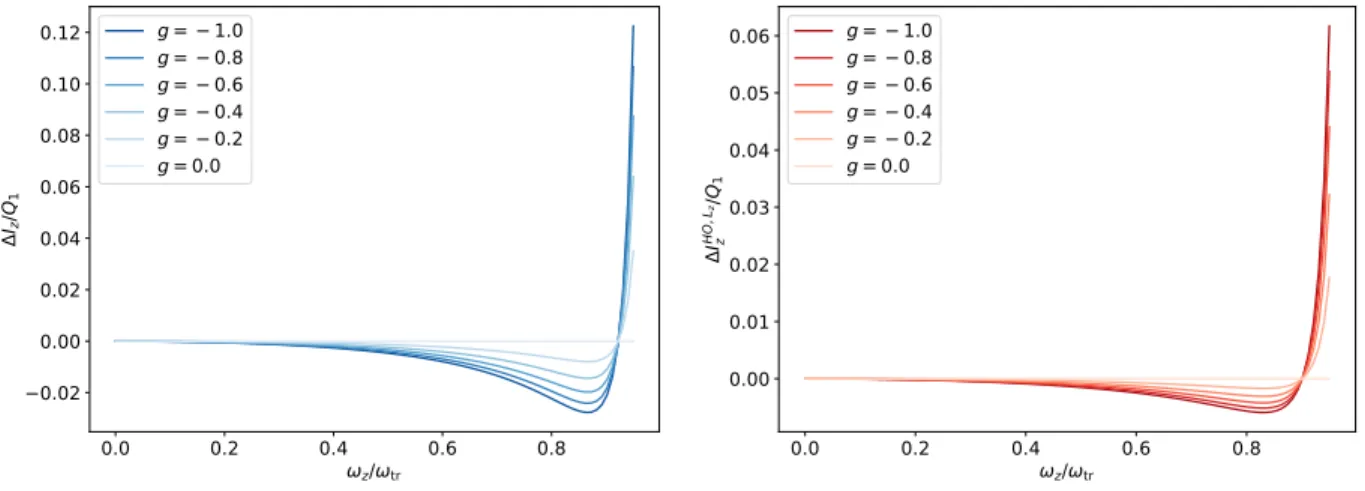
These results are shown in Figure 2.7 and Figure 2.8.
0.0 0.2 0.4 0.6 0.8
z/ tr 0.004
0.002 0.000 0.002 0.004 0.006
Lz /Q1
g = 1.0 g = 0.8 g = 0.6 g = 0.4 g = 0.2 g = 0.0
0.0 0.2 0.4 0.6 0.8
z/ tr 0.001
0.000 0.001 0.002 0.003
Lz /Q1
g = 1.0 g = 0.8 g = 0.6 g = 0.4 g = 0.2 g = 0.0
Figure 2.7: Change in the angular momentumhˆLzidue to the combination of rotation and repulsive contact interaction, for two
(left) and three (right) spatial dimensions, atz=e−2.0.
0.0 0.2 0.4 0.6 0.8
z/ tr 0.02
0.00 0.02 0.04 0.06 0.08 0.10 0.12
Iz /Q1
g = 1.0 g = 0.8 g = 0.6 g = 0.4 g = 0.2 g = 0.0
0.0 0.2 0.4 0.6 0.8
z/ tr 0.00
0.01 0.02 0.03 0.04 0.05 0.06
I
HO
,Lz
z
/Q1
g = 1.0 g = 0.8 g = 0.6 g = 0.4 g = 0.2 g = 0.0
Figure 2.8: Change in the moment of inertiahˆIzidue to the combination of rotation and repulsive contact interaction, for two (left)
and three (right) spatial dimensions, atz=e−2.0.
We can see also that the moment of inertia, while initially changing much more slowly than the angular momentum, starts to grow quickly in magnitude at the same point in rotation frequency where the angular momentum slows its growth, and then also changes direction and increases towards infinity at the phase transition.
Section 2.4: Summary and conclusions
In this chapter we have characterized the thermodynamics of a rotating Bose gase in 2D and 3D using the virial expansion. We implemented the SCLA, which allowed us to bypass solving then-body problem
to calculate then-th order virial coefficient [37].
In all cases, a finite angular velocityωzmodifies both the single-particle partition functionQ1as well as
the virial coefficients; the latter are further modified by the interactions. We have presented explicit formulas for the noninteracting case which do not appear elsewhere in the literature, to the best of our knowledge. As can be anticipated, the system becomes unstable atωz = ωtr, as the angular velocity allows particles to
escape the trapping potential in that limit. In that case, the virial coefficients remain finite, butQ1 diverges,
leading to divergent thermodynamics.
We have also obtained estimates to third order in the virial expansion for the angular momentumLz as
well as thez component of the moment of inertiaIz, as functions of the angular velocity0 < ωz < ωtrand
CHAPTER 3: Stochastic methods: from Markov chain Monte Carlo to Complex Langevin
Section 3.1: Quantum Monte Carlo methods
In order to treat quantum systems fully, we desire to move beyond approximate methods to ones which capture the behavior of the systems more generally, rather than in a limited set of regimes. Among the most popular methods for quantum many-body systems are quantum Monte Carlo (QMC) methods. This section provides an overview of these methods and illustrates them through discussion of the 2D Ising model.
Quantum Monte Carlo methods are a subset of Monte Carlo methods for quantum systems. In these methods, integrals (such as the path integral or the expectation value of the observables) are evaluated stochastically, yielding results that are exact up to some statistical uncertainty which depends on the number of samples used in the stochastic algorithm. This is done by means of a standard approximation scheme, where a generic integral of some function f(x)with weightp(x)
I=
Z b
a
dx p(x)f(x) (3.1)
can be approximated via a sum
IN = N
X
i=1
∆x f(xi)p(xi) (3.2)
where ∆x = bN−a. The exact integral is reproduced in the limit N → ∞. From this, is can be seen that increasingly accurate approximations can be achieved by increasing the size of N. In QMC, this N
corresponds to the number of samples taken in the algorithm. In most cases, evaluating an integral this way is inefficient, as the sort of integrals we wish to evaluate do not have uniform weight across paths. In fact, the weight (p(xi)in this notation, which corresponds to theeiS of Eq. (1.10) and Eq. (1.11)), is likely to be
significant in just a few high-probability regions. Use of an algorithm which focuses the sampling in those high-probability regions, therefore, will result in a much more efficient calculation.
probability depends only on the value immediately prior, i.e.
P(φn) = f(φn−1). (3.3)
This property allows for the generation of a set of random samples from a probability distribution via a sequential sampling process, making it an excellent technique for a computational algorithm. The use of these Markov chains is known as importance sampling, and – as implied by the name – improves the speed of our sampling by allowing us to generate configurations according to the probability distribution of the system, rather than sampling uniformly and weighting the configurations after the fact.
3.1.1: Importance sampling and the Ising model
A classic example from statistical physics of the usefulness of importance sampling algorithms is the Ising model. In 2D, the Ising model can be solved exactly, while in higher dimensions a stochastic solution is necessary. This makes this model a helpful point of comparison between stochastic algorithms and the known solution.
The 2D Ising model is a model for ferromagnetism in which spins are situated on an Nx×Nx lattice in
the presence of an external magnetic field. The Hamiltonian is
H =−JX
hi,ji
sisj−H N
X
i=1
si, (3.4)
where J is the strength of the spin coupling and H is the strength of the magnetic field multiplied by the
atomic magnetic moment. The partition function is
Z=X
i
e−βEi (3.5)
where β = 1
kBT and the energy of a single spin is calculated by summing over the nearest neighbors (n.n.):
Ei =−J si*.
, X
j∈n.n. sj+
H J
+ /
-. (3.6)
configuration is
E(α)=
Nx2 X
i=1
Ei (3.7)
and the magnetization of that configuration is
M(α) =
N2 x X
i=1
Mi (3.8)
Mi = µsi. (3.9)
We can see from this description of the magnetization that it depends on the average direction of the spins. If the spins are largely aligned in the same direction, we find a nonzero magnetization for that configuration, whereas in a randomly-aligned system, we expect the magnetization to be zero.
The average energy and magnetization are computed by summing over all possible spin configurations of the lattice in the following way:
hEi = 1
Nα
X
α
E(α) (3.10)
hMi = 1
Nα
X
α
M(α) (3.11)
whereE(α)andM(α)come from Eq. (3.7) and Eq. (3.8).
Since the total number of possible lattice configurations Nα scales exponentially in lattice size (Nα ∝ 2N2
x), for even moderately-sized lattices (Nx > 4), we need to use a stochastic algorithm that prioritizes
sampling from high-probability configurations. This is where importance sampling comes in.
The importance sampling algorithm most often used with the Ising model is the Metropolis-Hastings algorithm, which uses a random walk in configuration space paired with an accept-reject step to guide the sampling towards higher-probability regions. In this case, what that means is that the algorithm proceeds as follows:
1. Initialize the lattice with some random configuration of spins (+1for up and−1for down) 2. Calculate the total energy of this spin configuration (using Eq. (3.7))
4. Calculate the energy of this new configuration (again using Eq. (3.7))
5. Determine the ratio of the probability of this new configuration to the old one
P(α) = 1
Ze
−βE(α) (3.12)
P(αnew)
P(αold) =
e−β(E(αnew)−E(αold) (3.13)
6. Accept or reject the new configuration by comparing this ratio to a random number generated uniformly in the range(0,1).
7. If the new configuration is as probable or more probable than the random number, keep the new lattice configuration. Otherwise, revert to the previous configuration, choose a new spin to flip, and repeat the process outlined above
The algorithm continues untilNαspin configurations have been collected. The energy and magnetization of these configurations are the samples, which we average together according to Eq. (3.10) to get our average values.
3.1.2: Limitations of quantum Monte Carlo algorithms
The previous section relied upon the important assumption that the quantity weighting our observables (e−βE in this case andeiS more generally) was positive definite. This allows is to treat the quantity like a
probability, and use it to guide our Markov chain. But what happens when we can no longer rely on this assumption? This is an example of the sign problem arising in quantum lattice calculations.
This is where alternative stochastic methods can help. The remainder of this chapter focuses on the stochastic method known as complex Langevin, which can be utilized to circumvent the sign problem. Section 3.2: Complex Langevin: origins and method