Estimation and optimization of the performance of polyhedral process networks

(1)

Cover Page

The handle http://hdl.handle.net/1887/22911 holds various files of this Leiden University

dissertation.

Author

: Haastregt, Sven Joseph Johannes van

Title

: Estimation and optimization of the performance of polyhedral process networks

(2)

Estimation and Optimization of

the Performance of

Polyhedral Process Networks

(3)

(4)

Estimation and Optimization of the Performance of

Polyhedral Process Networks

Proefschrift

ter verkrijging van

de graad van Doctor aan de Universiteit Leiden,

op gezag van Rector Magnificus prof.mr. C.J.J.M. Stolker,

volgens besluit van het College voor Promoties

te verdedigen op dinsdag 17 december 2013

klokke 12:30 uur

door

Sven van Haastregt

geboren te Rijpwetering

(5)

Samenstelling promotiecommissie:

promotor Prof.dr. Ed Deprettere co-promotor Dr. Bart Kienhuis

overige leden: Prof.dr. Joost Kok Prof.dr. Harry Wijshoff

Prof.dr. Koen Bertels Technische Universiteit Delft Dr. Hristo Nikolov

This manuscript was edited by the author using Vim, and typeset using LA_{TEX 2}_ε_,

BIBTEX, andMakeIndex in a process automated using GNU Make. Graphics were

produced mostly using Inkscape, and occasionally using Xfig or gnuplot. Git over ssh was used for revision tracking, synchronization, and backup purposes.

Cover design by Marcel IJssennagger.

Estimation and Optimization of the Performance of Polyhedral Process Networks Sven van Haastregt.

-Thesis Universiteit Leiden. - With index, ref. - With summary in Dutch 190 pages, 47988 words, 176 index entries, 162 references.

ISBN 978-94-6182-383-0

Copyright c2013 by Sven van Haastregt, Leiden, The Netherlands.

All rights reserved. No part of the material protected by this copyright notice may be reproduced or utilized in any form or by any means, electronic or me-chanical, including photocopying, recording or by any information storage and retrieval system, without permission from the author.

(6)

(7)

(8)

C

ONTENTS

Contents vii

Notation xi

1 Introduction 1

1.1 Problem Context . . . 1

1.2 Problem Statement . . . 4

1.3 Related Work . . . 7

1.3.1 High-Level Synthesis . . . 8

1.3.2 Electronic System-Level Synthesis. . . 10

1.4 Contributions and Outline. . . 12

2 Background 15 2.1 Polyhedral Model . . . 15

2.2 Models of Computation . . . 21

2.2.1 Homogeneous Synchronous Dataflow . . . 22

2.2.2 Synchronous Dataflow . . . 23

2.2.3 Cyclo-Static Dataflow . . . 25

2.2.4 Polyhedral Process Networks . . . 27

2.3 Derivation of PPNs from Sequential Programs . . . 30

2.3.1 Channel Type Determination . . . 31

2.3.2 Buffer Size Computation . . . 32

2.4 Code Generation . . . 33

2.4.1 Integrating Dedicated IP Cores . . . 34

3 Synthesizing PPNs 37 3.1 Motivation & Contributions. . . 37

3.2 IP Core Characterization . . . 38

(9)

viii _Contents

3.3 Data Reuse . . . 40

3.4 Sticky FIFOs . . . 42

3.5 Evaluation Logic Optimizations . . . 43

3.5.1 Pipelined Evaluation Logic. . . 44

3.5.2 ROM-Based Evaluation Logic . . . 44

3.5.3 Related Work . . . 47

3.6 Out-of-Order Communication . . . 48

3.7 Conclusion and Summary. . . 52

4 Performance Estimation 53 4.1 Motivation. . . 53

4.2 Definitions. . . 55

4.3 RTL Simulation . . . 57

4.4 SystemC Simulation . . . 57

4.4.1 Cycle-Accurate Timed SystemC Simulation . . . 58

4.4.2 Light-weight Timed SystemC Simulation . . . 60

4.5 Maximum Cycle Mean Analysis . . . 61

4.5.2 Maximum Cycle Mean Analysis . . . 63

4.5.3 Derivation of PPN Modeling Graphs. . . 64

4.5.4 Case Studies . . . 72

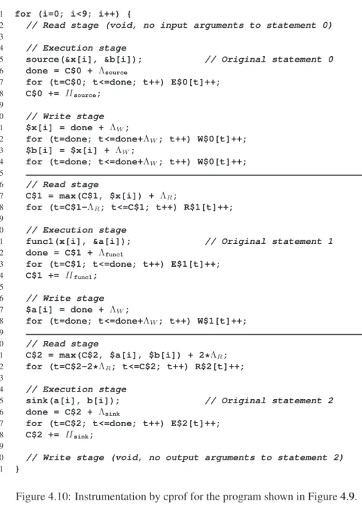
4.6 Sequential Code Profiling . . . 75

4.6.2 Sequential Code Instrumentation of Static Programs . . . . 77

4.6.3 Maximum Degree of Parallelism . . . 84

4.6.4 Absolute Throughput Estimation . . . 85

4.6.5 Case Study . . . 85

4.6.6 Transformation Performance Estimation . . . 90

4.6.7 Instrumentation Overhead . . . 92

4.7 Comparison . . . 94

4.8 Experimental Results . . . 96

4.8.1 Accuracy . . . 97

4.8.2 Running Time . . . 98

5 Application Transformation 101 5.1 Transformations. . . 101

5.1.1 Splitting. . . 101

(10)

Contents ix

5.1.3 Stream Multiplexing . . . 106

5.1.4 Scheduling . . . 109

5.2 Transformation Efficacy Analysis . . . 116

5.2.1 Splitting . . . 116

5.2.2 Merging . . . 120

5.2.3 Stream Multiplexing . . . 121

5.2.4 Scheduling . . . 124

6 Industrial Case Study 129 6.1 Sphere Decoding . . . 129

6.2 Reference Implementation . . . 131

6.3 AutoESL . . . 132

6.3.1 Design Flow . . . 133

6.3.2 Design Entry . . . 134

6.3.3 Design Productivity . . . 138

6.4 Daedalus . . . 140

6.4.1 Design Entry . . . 141

6.4.2 Synthesis . . . 147

6.5 Comparison . . . 148

7 Conclusions 151

Samenvatting 155

Curriculum Vitae 157

Acknowledgments 159

Bibliography 161

(11)

(12)

N

OTATION

| · | Cardinality:|S| ≡the number of elements inS, page20.

[·,·) Interval:[a, b) ={x∈Z|a≤x < b}.

⌈·⌉ Least integer:⌈x⌉=n⇔n∈N∧n−1< x≤n.

· ≺ · Lexicographical order, page18.

Dp Iteration domain of processp, page27.

d(e) Number of initial tokens on edgee, page22.

δc Process reading from channelc, page27.

E The set of channels of a PPN, page27.

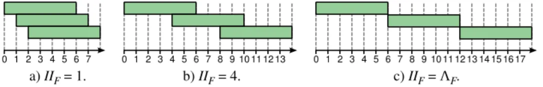
IIF Initiation interval of functionF, page38.

IPDk_i k-th Input Port Domain of processi, page27.

ΛF Latency (input-to-output delay) of functionF, page38.

Mc Channel relation of channelc, page27. N The set of natural numbers, including 0.

N+ The set of positive natural numbers, excluding 0.

OPDk_i k-th Output Port Domain of processi, page27.

P The set of processes of a PPN, page27.

Q The set of rational numbers.

σc Process writing to channelc, page27.

Tp Period of a processp, page55.

t(a) Execution time of data flow nodea, page22.

τp Throughput of a processp, page55.

θ(i) Application of scheduleθto iteration vectori, pages111,112.

(13)

(14)

CHAPTER

1

I

NTRODUCTION

E

LEMENT NUMBER14, or silicon, has been important for many ancient civiliza-tions, albeit mostly as a constituent of sand and rocks. Silicon was essential for the construction of houses, temples, and roads, which together formed the cen-ters of society. In 1954, a new and very different use for silicon was found that would have a dramatic impact on the established centers of society: Gordon Teal and his team produced the first silicon transistor [Che04]. Many electronic devices have become available since then, in which silicon transistors are an essential com-ponent. By miniaturization, more and more transistors could be fit onto a small area, thereby enabling the construction of complex processing systems. Contemporary examples of such processing systems include the special purpose processors found in automotive, mobile communications, medical, industrial, and entertainment ap-plication domains. Many of these processing systems are tightly coupled to their environment and perform a specific task, and are therefore classified asembedded systems[LS11,Mar11,SB00]. Central to this dissertation is the design of the special purpose processors in these embedded systems.

1.1 Problem Context

(15)

2 _{Chapter 1. Introduction}

embedded systems. Such MPSoCs consist of many different components such as programmable processing components, specialized processing components, memory components, and input/output interfaces. By letting multiple components work in parallel, the demand for computational power is met. Unfortunately, the design of an MPSoC is even more challenging than the design of a single-processor system. The challenge for the designer is to distribute computations over different processors of the MPSoC. While doing so, the designer should guarantee functional correctness of the system and at the same time make tradeoffs between orthogonal design aspects such as circuit area and performance [Mar06]. Thus, the shift to multi-processor sys-tems may address the demand for computational power, but this comes at the expense of a further increase in design complexity.

Traditionally, processors have been designed at theRegister Transfer Level(RTL). An RTL specification of a processor consists of registers that are interconnected by signals and combinational logic. RTL design of modern MPSoCs is becoming in-creasingly error-prone and time-consuming because of the abundance of registers, signals, and combinational logic needed for a modern MPSoC’s functionality. To cope with the design complexity of modern MPSoCs, the designer needs to work at a level of abstraction above the RTL. This has led to the emergence of Elec-tronic System-Level(ESL) design methodologies [GAGS09,BM10]. In such a design methodology, the designer first specifies a system at a high level of abstraction. Next, the designer constructs an RTL implementation from the initial specification with the aid of system-level design automation tools.

An example system-level design tool set is the open-source Daedalus tool set which has been developed at the Leiden Embedded Research Center (LERC) [NSD08b,

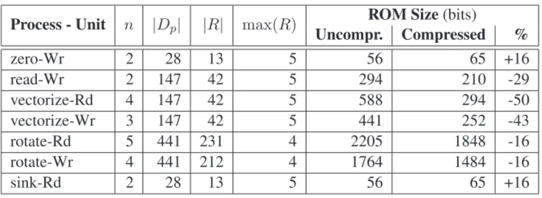
Lei08]. We leverage the Daedalus tool set in this thesis. This means that we want to develop the special purpose processors of an embedded system with Daedalus. An overview of the Daedalus system-level tool flow is depicted in Figure1.1. Daedalus enables a designer to obtain a deployable gate-level specification from a system-level specification in a fully automated way. The functional behavior of the system-level specification is specified as a sequential C program, as shown at the upper right part of Figure 1.1. The elaboration from one specification level to a lower specification level is done in a fully automated way. We discuss the different aspects of Daedalus in the following paragraphs.

(16)

Sec-1.1. Problem Context 3

P µ

P

µ µP

System−level specification specification

Validation / Calibration Gate−level

specification RTL specification Mem Mem HW IP MPSoC connectInter− Functional Mapping spec. in XML Sequential program in C

Library IP components

RTL Models Models High−level

Platform spec.

Automated system−level synthesis: Espam

Platform IP cores

processors

Auxiliary PNgen Parallelization: System−level design space exploration:

Sesame

Manually creating a PPN

Polyhedral Process Network in XML

in VHDL

Application spec. in XML

code for C

netlist files

Low−level synthesis: e.g. Xilinx Platform Studio, XST

Figure 1.1: Daedalus system-level tool flow overview [NSD08b].

ond, an imperative specification assumes shared memory which is likely to become a performance bottleneck on a multi-processor system. A distributed memory model better matches a multi-processor system, but it is not possible in the general case to extract a distributed memory model from an imperative specification.

(17)

Various approaches exist to bridge the specification gap. One approach is to ex-tend a sequential program with library calls or compiler pragma directives to indicate tasks that can execute concurrently. Examples of this approach include pthreads, OpenCL [Khr08], and OpenMP [Ope97]. Another approach is to automatically ex-tract concurrent tasks from a sequential program using a parallelizing compiler such as LooPo [GL97], Polaris [BEF+94], Pluto [BBK+08], or PNGEN[VNS07]. The latter is part of Daedalus to bridge the specification gap. PNGENgenerates a parallel specification from a sequential program written in a subset of the C language. We discuss PNGENin more detail in Section2.3.

A system-level specification lacks many details that are present in the RTL speci-fication because these details are irrelevant at the system level. For example, at the system level the designer reasons about sending data from one processor to another without specifying the registers and logic that implement such communication in the RTL specification. Not exposing the designer to such implementation details allows a designer to better cope with complex systems. However, the omission of imple-mentation details opens up a gap between the system-level specification and the RTL implementation, which is known as theimplementation gap[NSD08b]. To obtain a functional implementation from a system-level specification, the implementation gap needs to be bridged by adding low-level implementation details to the system-level specification. This is done by a level synthesis tool which refines a system-level specification into an RTL specification in a systematic and automated way.

The Daedalus tool set provides the ESPAMtool for automated system-level

synthe-sis. A system-level specification for ESPAMis composed of three individual

specifi-cations: an implementation platform specification describing the number and types of processing and interconnect components of the system; a parallel application specifi-cation consisting of a network of communicating tasks; and a mapping specifispecifi-cation that maps the application tasks onto processing components. The ESPAM tool gen-erates an RTL specification from the three specifications. This RTL specification is then taken through commercial low-level synthesistools that convert the RTL into a gate-level specification. Place-and-route tools take such a gate-level specification and create a layout of the circuit which can be implemented on aField-Programmable Gate Array(FPGA) or provided to anApplication-Specific Integrated Circuit(ASIC) manufacturing process. This last step yields a complete MPSoC implementation.

1.2 Problem Statement

(18)

1.2. Problem Statement 5

a working prototype of a system in only a few hours of time [NSD08b]. However, many different implementations of an application specification are possible that have identical functionality but differ in performance and implementation cost aspects. This presents the designer with another problem: selecting an implementation from a vastdesign spaceof possible implementations. Only a subset of thedesign points in this design space represent implementations that satisfy a set of givendesign con-straintson performance and circuit area. Thus, solely closing the specification and implementation gaps still leaves open the problem of selecting the design point that best matches a set of design constraints.

A Daedalus system-level specification consists of the application, platform, and mapping subspecifications, as described in the previous section and shown in Fig-ure1.1. Each of these subspecifications may be transformed to yield a functionally equivalent implementation that has different performance and resource cost prop-erties, as described by the Y-chart approach [KDWV02]. For example, a designer can transfrom the platform specification by adding or removing processors, or trans-form the mapping specification by moving a task from one processor to another, or transform the application specification by splitting a tasks into smaller subtasks and thereby exposing more parallelism. Many combinations of suchtransformationsare possible and this number grows rapidly as application and platform sizes increase. As a result, the design space for a modern MPSoC is typically very large.

Despite the existence of fully automated system-level synthesis tools, implementing and evaluating all design points is infeasible for modern MPSoC design because of the large design space. Therefore, the design space should be explored in such a way that only the “promising” design points need to be implemented and evaluated. Find-ing the promisFind-ing design points is a non-trivial multi-objective optimization problem. ManyDesign Space Exploration(DSE) techniques have been proposed to efficiently search large design spaces [Gri04]. Daedalus incorporates the SESAMEDSE tool to

explore the design space using an evolutionary algorithm [PEP06]. SESAMErelies on

trace-based simulation to estimate the performance of candidate design points. Al-though SESAME’s simulation is intended for fast performance analysis, conducting many simulations may still take a considerable amount of time [PP12]. This leads to unreasonably long design times.

(19)

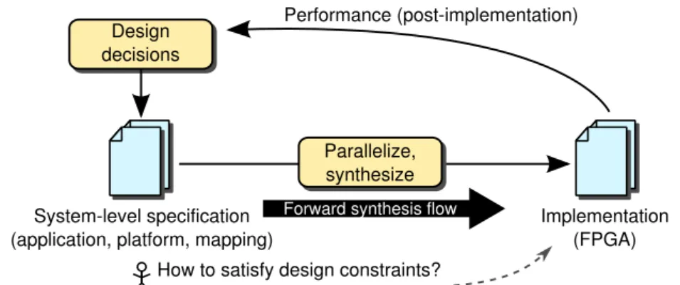
System-level specification (application, platform, mapping)

Implementation (FPGA) Performance (post-implementation) Design

decisions

Parallelize, synthesize

How to satisfy design constraints? Forward synthesis flow

Figure 1.2: Iterative system-level design flow.

implementation gap. If a performance constraint is not satisfied, the system-level specification is transformed based on performance and cost metrics obtained from the prototype implementation. These transformations entail modifying the application by rewriting the C code, modifying the platform by adding processors, or modifying the mapping by assigned tasks to different processors. The designer relies on experience and expertise to come up with transformations that most likely have the desirable effect on performance and cost aspects. Building up this knowledge is referred to as the “acquisition of insight” [Spe97]. However, it is not trivial to predict beforehand if and by how much a certain transformation affects performance and cost aspects. At this moment, the best a designer can do is to perform a new time-consuming synthesis step after transforming the system-level specification. This procedure is repeated un-til an implementation is obtained that satisfies performance constraints. The designer can then proceed with the actual manufacturing of the system.

A naive iterative design flow may appear to be more deterministic than a random-search driven DSE flow. Because the designer iteratively transforms a system-level specification in a pragmatic manner, a system that satisfies all performance con-straints should eventually be the result. However, this only holds if the designer always makes the optimal decisions. This does not always happen in practice, be-cause the designer may for example overlook solutions or ignore solutions that seem counter-intuitive. Another problem with a naive iterative design flow is that evalua-tion of a single specificaevalua-tion may easily take a few hours of time. This reduces the number of iterations a designer can make in a given time frame, increasing time-to-market.

(20)

1.3. Related Work 7

synthesis tools. However, it does not address the following problem: given a perfor-mance constraint, which transformations should the designer apply to obtain an im-plementation that meets this performance constraint? For example, consider the sce-nario in which a designer constructs a video processing system under the constraint that the system should meet a throughput of 20 frames per second. After synthesiz-ing the system-level specification, the designer finds that the system works at only 11 frames per second. This puts a burden on the designer to transform the system-level specification such that the performance constraint of 20 frames per second is met. We therefore argue that solely bridging the specification and implementation gaps is not sufficient to solve a design problem.

In this dissertation, we consider the iterative system-level design flow of Figure1.2

and address a designer’s problem that is currently not addressed. That is, we ask how to modify this design flow to obtain a constraint-satisfying implementation of a system in a short amount of time. This modification is needed as synthesizing a design in the current flow takes too long, keeping the designer in the dark whether the design will satisfy the designer’s constraints. Performance estimation methods are lacking that could provide an early indication of whether a design will satisfy the designer’s constraints at all. After obtaining an implementation not meeting the constraints, there is little guidance to help a designer transform his design in such a way that his performance constraints will be satisfied. In this context, we formulate our three central research problems as follows:

1. Synthesis: How to automatically obtain efficient RTL implementations from a high-level specification that enable application of established transformations such as splitting, merging, stream multiplexing, and scheduling?

2. Performance estimation: How to assess the absolute performance of a de-sign point, possibly in different ways by trading off evaluation speed against accuracy?

3. Optimization: How to obtain an implementation that satisfies a performance constraint while reducing the number of design iterations?

Only after addressing these three problems from a designer’s perspective, Daedalus can become a powerful system-level synthesis tool capable of solving design prob-lems.

1.3 Related Work

(21)

Daedalus methodology addresses the problem of obtaining an efficient FPGA im-plementation from a high-level application specification in a short amount of time. As such, Daedalus provides an important stepping stone to address the three central problems, ultimately leading to an extended Daedalus design flow that also considers performance constraints.

Daedalus is only one of many methodologies to (semi-)automatically obtain special purpose processor implementations from high-level application and system specifi-cations. In this section, we give a brief overview of related approaches to obtain RTL implementations from high-level application specifications. We discuss related high-level synthesis techniques in Section 1.3.1and related electronic system-level synthesis techniques in Section 1.3.2. Related work specific to each of the three central problems is discussed separately in Chapters3,4, and5.

1.3.1 High-Level Synthesis

Automated synthesis of RTL implementations from specifications above the register transfer level, known as High-Level Synthesis (HLS), has been subject of research since the late 1980s [MK88,MPC88,PK89]. Since then, many academic and mercial HLS tools have been developed. In 1994, electronic design automation com-pany Synopsys released its Behavioral Compiler tool that is widely regarded as the first commercial HLS tool [CM08]. This tool took a behavioral description of a de-sign in VHDL or Verilog as input and generated a cycle-accurate VHDL or Verilog description. During synthesis, the tool allowed the designer to trade off throughput against chip area. Since then, many different HLS tools have been released by dif-ferent companies, with varying degrees of commercial success. As of 2013, three of the major commercially available HLS tools are Synopsis SynphonyC [Syn10], Xilinx Vivado HLS [Xil13], and Calypso Catapult [Cal11]. A difference with Be-havioral Compiler is that modern commercial HLS tools have anchored on C, C++_,

or SystemC input specifications instead of input specifications using Hardware De-scription Languages like VHDL or Verilog [Fin10]. Meeus et al. conducted a com-parison between twelve different commercial and open-source high-level synthesis tools [MVBG+12].

(22)

1.3. Related Work 9

interconnect them manually using communication primitives. Advanced compilation techniques such as those employed by Daedalus allow tools to automatically derive such interconnects from a sequential specification. The ROCCC tool takes a subset of the C language as input and generates RTL targeted towards FPGAs [GNB08]. ROCCC requires that loop iterators are used in at most one array dimension. This poses a problem when expressing for example a loop skewing transformation. Such a restriction is not necessary in Daedalus as any affine expression of loop iterators is an-alyzable using the polyhedral model. Other HLS approaches that employ the polyhe-dral model include for example PARO [HRDT08] and MMALPHA[GQR03]. These approaches use functional languages as input, while commercial tools and Daedalus all use an imperative language. Related early work included modeling affine nested loop programs using uniform recurrence equations to generate systolic array imple-mentations [Qui84]. The FCUDA approach takes C code annotated using NVIDIA’s CUDA primitives and generates C code annotated with AutoESL pragmas to obtain an FPGA implementation [PGS+09]. This allows a designer to express parallelism in a single specification and target both GPU and FPGA platforms. Besides the main FPGA backend, Daedalus also includes a GPU backend, allowing a designer to also target both GPU and FPGA platforms. Unlike FCUDA, Daedalus does not require CUDA-like annotations of the C code.

High-level synthesis should not be confused with design entry using a high-level language, because the use of a high-level language does not necessarily imply that the design is specified at a high level of abstraction. For example, Handel-C is a subset of the C language with extensions to describe hardware succinctly [Pag96]. Parallel behavior is expressed using the Communicating Sequential Processes (CSP) model of computation [Hoa85]. Similar to RTL design, the designer should per-form scheduling and pipelining manually, whereas this is perper-formed automatically in an HLS flow. Cobble is a language similar to Handel-C [TCL05] with support for custom compilation schemes. This allows a designer to define how a particular pattern in the source program should be mapped to hardware. Cobble is compiled into Pebble, which is a simplified hardware description language supporting design parameterization and run-time reconfiguration [LM98]. MyHDL allows a designer to specify hardware in the Python language [Dec03]. MyHDL still requires the designer to specify the behavior of the hardware at the register-transfer level using constructs provided by the MyHDL Python package.

(23)

the data path [NSD08a]. Moreover, Daedalus generates complete heterogeneous MP-SoC implementations, which is a task that is beyond the scope of high-level synthe-sis. Another difference between HLS tools and Daedalus is the model used to rep-resent applications. HLS tools predominantly employ Control Data Flow Graphs (CDFGs) [MPC88,CGMT09], whereas Daedalus employs a process network based model [VNS07].

1.3.2 Electronic System-Level Synthesis

(24)

1.3. Related Work 11

Daedalus, MAPS does not provide an automated way to obtain a parallelized variant of a sequential application. The Multi-Application and Multi-Processor Synthesis (MAMPS) flow maps synchronous dataflow graphs onto homogeneous MPSoCs. In contrast, Daedalus uses the more expressive PPN model and targets heterogeneous MPSoCs. MAMPS on the other hand supports multiple applications at once, whereas the Daedalus version used in this thesis supports only one application at once, al-though the DaedalusRTextension does support multiple applications [BZNS12].

Bluespec SystemVerilog (BSV) is a high-level hardware description language in-tended to describe complete systems [NC10]. In a comparison conducted by Nikolov et al., a C specification of an H.264 video decoder was implemented using both the automated Daedalus flow and as a semi-custom design in BSV [NRD+09]. The Dae-dalus design employed programmable components as processing elements, on which the C specification was mapped. The Bluespec design employed dedicated hardware processing elements, requiring manual conversion of the C specification to BSV. The authors found that the design time for the Daedalus approach was roughly 6 times shorter than the design time for the Bluespec design. This difference was mainly caused by the manual conversion and verification in the BSV design. However, the shorter design time in Daedalus came at the expense of higher resource cost caused by the use of programmable processors. Replacing programmable processors with dedicated RTL cores may reduce the resource cost footprint in the Daedalus flow. Such cores can be obtained automatically from C using HLS tools. We discuss the integration of HLS in Daedalus in Chapter3.

Several ESL tools focus on graphical entry of a system-level design. For example, a system is specified in Koski using Unified Modeling Language (UML) [KKO+06]. Xilinx System Generator provides a block-based design environment [Xil02]. A Sys-tem Generator design can be compiled into a netlist, which can then be synthesized onto an FPGA. The latest Vivado design suite from Xilinx integrates System Gener-ator, AutoESL, and RTL synthesis into a single ESL design environment.

(25)

anal-12 _{Chapter 1. Introduction}

ysis techniques such as Banerjee’s test [Ban88]. But as a result of the approximate nature, tools may need to conservatively assume a data dependence exists between statements, possibly preventing any parallel execution. Such false data dependences can be circumvented using tool-specific compiler pragmas that need to be inserted by the designer. Daedalus requires that the application is specified as a SANLP (cf. Section2.3) for which exact data dependence analysis is always feasible. This elim-inates the need for conservative data dependence assumptions, freeing the designer from having to manually analyze data dependences.

1.4 Contributions and Outline

In Section 1.2, we identified three central problems in an iterative system-level de-sign flow. We solve these three problems in this dissertation in the context of the Daedalus methodology [NSD08b], which we discuss in more detail in Chapter 2. The Daedalus methodology is the result of many dissertations in the LERC group [Rij02,Ste04,Tur07,ZI08,Nik09,Mei10,Nad12,Bal13]. We want to build further upon the contributions made in these dissertations. The research conducted in this thesis has led to the following four contributions:

Contribution I[HK09,NHS+11,HK12]: As a solution to the synthesis problem, we add extensions to the Daedalus methodology. These extensions enable us to obtain FPGA implementations from C programs which were already accepted by Daedalus, but for which an FPGA implementation was not yet feasible. With these extensions, we are now able to obtain complete FPGA implementations for industrially relevant applications, like the sphere decoder application discussed in Chapter 6. We have shown that we can characterize and integrate functional kernels (IP cores) from a broad set of conventional HLS tools like the industrial tools Vivado HLS and Syn-phony C, and the academic tool DWARV. Our extensions to the Daedalus methodol-ogy provide an enabling step to realize the complete conventional “forward” system-level synthesis flow for FPGAs in the flow shown in Figure1.3. The position of these extensions is indicated by the➊_{in Figure}_1.3_{and are discussed in}_Chapter₃_.

(26)

an-1.4. Contributions and Outline 13

System-level specification (application, platform, mapping)

Implementation (FPGA) Performance (post-implementation) Design

decisions

Parallelize, synthesize

How to satisfy design constraints? Forward synthesis flow

1 2

3

Performance Heuristics

Extensions

Figure 1.3: Contributions positioned in the iterative design flow.

other contribution of this thesis iscprof, which is a novel profiling based approach that completely bypasses the forward synthesis flow. The approach is robust as it relies only on an ordinary C++_{compiler to obtain accurate performance estimates of}

PPNs. Moreover, the approach allows for early estimation of the effects of transfor-mations. The approach provides the designer with an upper bound on the degree of parallelism in an application specification. This allows a designer to assess at a very early stage in the design flow whether he can meet his constraints. The position of the alternative performance estimation techniques in the overall design flow is indicated by the➋_{in Figure}_1.3_{and is discussed in}_Chapter₄_.

Contribution III[HK12]: As a solution to the optimization problem, we provide heuristics to optimize a design by leveraging the insight gained from the performance estimation techniques discussed in Chapter4. The heuristics provide a concrete set of criteria that guide the designer in selecting standard transformations such as split-ting, merging, stream multiplexing, and scheduling. This position of the heuristics is indicated by the➌_{in Figure}_1.3_{and is discussed in}_Chapter₅_.

Contribution IV[HNVK11, NNH+10, NNH+11]: We have shown that we can apply the extended forward system-level synthesis flow depicted in Figure1.3on an industrially relevant application. This case study also shows that PPNs are a feasible alternative to conventional CDFG-based C-to-RTL flows. Using the heuristics from Chapter 5, in particular merging, we were able to transform the design to obtain a new pareto design point that was not achievable with a state-of-the-art industrial HLS tool. The use of the profiling-based cprof performance estimation technique presented in Chapter4was essential to gain insight in the application performance and the optimization opportunities. The case study is discussed inChapter6.

(27)

(28)

CHAPTER

2

B

ACKGROUND

In this chapter, we introduce concepts and notations that are used throughout this thesis. In Section2.1, we introduce the polyhedral model which we employ for anal-ysis of programs. In Section2.2, we review various models of computation that are widely employed to represent applications. We focus on the polyhedral process net-work model of computation employed by Daedalus and review in Section2.3 how such networks can be derived from a particular class of sequential programs. In Section2.4, we review how processes of polyhedral process networks can be imple-mented in hardware.

2.1 Polyhedral Model

(29)

16 _{Chapter 2. Background}

0 1 2 3 4 5

Upper half-space

Lower half-space

Figure 2.1: A 1-dimensional hyperplane (i.e., a line) H1 = {(j, i) ∈ Q2 | i = 3}

dividing a 2-dimensional space.

in the polyhedral model. A polyhedron can be defined using hyperplanes.

Definition 2.1(Hyperplane).

AhyperplaneHis a subspace of dimensiond−1inside ad-dimensional space, that is,

H ={x∈Qd|aTx=c},

whereais a non-zero vector of sizedandcis a constant [Rij02].

A hyperplane is a generalization of a conventional 2-dimensional plane to n ∈ N

dimensions. A 1-dimensional hyperplane dividing a 2-dimensional space is shown in Figure 2.1. A hyperplane divides a space into an upper and a lower half-space. We distinguishopen half-spaceswhich do not include the dividing hyperplane itself, andclosed half-spaceswhich include the dividing hyperplane. We use hyperplanes to define subspaces ofQd, known as rational polyhedra:

Definition 2.2(Rational Polyhedron).

A rational polyhedronP is a subspace ofQd that is bounded by a finite set of m

hyperplanes, that is,

P ={x∈Qd|Ax≥c},

whereAis an integralm×dmatrix andcis an integral vector of sizem[Ver10].

(30)

2.1. Polyhedral Model 17

a) Rational polyhedron. b) Rational polytope.

0 1 2 3 4 5

e) Statement with modulo guard. for (j=2;j<=5;j++) { for (i=1;i<=6-j;i++) { F(...);

} }

c) Loop nest represented by b).

for (j=2;j<=5;j++) { for (i=1;i<=6-j;i++) { if (i%2 == 0) F(...); }

}

for (j=2;j<=N;j++) { for (i=1;i<=6-j;i++) { F(...);

} }

d) Loop with parametric bound.

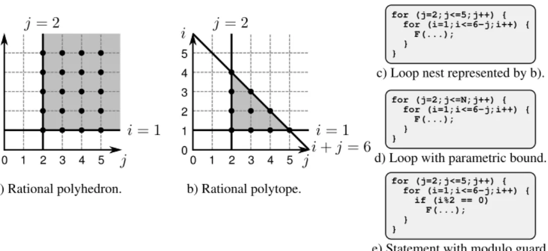
Figure 2.2: a) A 2-dimensional rational polyhedron; b) a 2-dimensional rational poly-tope; c) a loop nest of depth two that can be represented by the 2-dimensional ratio-nal polytope given in b); d) a loop nest where the outer loop has a parametric upper bound; and e) a statement with a modulo guard.

Definition 2.3(Parametric Rational Polyhedron).

Aparametric rational polyhedronP(s)is a family of rational polyhedra inQdthat is parametrized by parameterss∈Qn:

s7→ P(s) ={x∈Qd|Ax+Bs≥c},

whereA is an integral m ×dmatrix, B is an integral m×nmatrix, and c is an integral vector of sizem[Ver10].

A parametric rational polyhedron can represent a loop nest that iterates over a finite, possibly parameterized set of iterations. By assuming that the iterators of such a loop nest are integers, we can represent a loop nest as a set of integral points in a (parametric) rational polyhedron. For example, the loop nest shown in Figure2.2c can be represented by the rational polytope shown in Figure2.2b. Each iteration of the loop nest has a corresponding point in the rational polytope. The loop nest shown in Figure2.2d can be represented by a parametric rational polytope.

When for example a statement is guarded with an expression containing a modulo operator, we are interested in only a subset of the points of a parametric rational polyhedron. In the example shown in Figure2.2d, functionFis called only for even values of iteratori. We define the polyhedral set to represent a subset of points in a

(31)

3 4 5

0 1 2 3 4 5

6 7 8 9 10

S =

(

(j, i)∈Z2_{| ∃} e∈Z:



   

−1 0

1 0

0 1

−1 −2

     · j i +      2 −2 0 0 0     

·(e)≥      0 0 4 1 −12      )

= {(j, i)∈Z2

| ∃e∈Z: 2e=j∧j≥4∧i≥1∧

2i+j≤12}

Figure 2.3: Example polyhedral set.

Definition 2.4(Polyhedral Set).

Apolyhedral setSis a finite union of basic integer sets,S = S

iSi, of typeQn →

2Qd

, where each basic integer setSiis defined as

Si =s7→ Si(s) ={x∈Zd| ∃z∈Ze:Ax+Bs+Dz≥c},

whereAis an integralm×dmatrix,Bis an integralm×nmatrix,Dis an integral

m×ematrix, andc is an integral vector of sizem. The parameter domain ofS,

{s∈Zn_{| S}₍_s₎₆₌_∅}_{, is a polyhedral set containing all parameter values}_s_{for which}

S is non-empty. A polyhedral set with an empty parameter domain (i.e., n = 0) is called a non-parametric polyhedral set, and denoted with “s 7→” omitted. The parameter domain of a polyhedral set is always non-parametric [Ver10].

The polyhedral set depicted in Figure 2.3 contains only a subset of the integral points of its bounding rational polytope. In particular, it only contains the integral points for even values of j, which can be expressed as “j mod2 = 0”. Such con-straints are enforced using the existentially quantified variables zin Definition 2.4. For example, the constraint “jmod2 = 0” is represented by a condition2e=jand the requirement thateis integral.

To allow reasoning about the execution order of different iterations of a program, we define the lexicographic order on the points of a polyhedral set:

Definition 2.5(Lexicographic Order).

(32)

2.1. Polyhedral Model 19

ai < bifor the first dimensioniin which both elements differ, or, equivalently,

a≺b≡

n

_

i=1



ai< bi∧ i−1

^

j=1

aj =bj



.

For example, an elementa= (2,3,5)is lexicographically smaller than an element

b = (2,4,0), because the first difference between both elements is in the second dimension, and the value 3 in the second dimension ofais less than the value 4 in the second dimension ofb.

Loop optimizations such as skewing transform iteration domains that we represent using polyhedral sets. A transformation of a polyhedral set can be expressed as a relation between the original polyhedral set and the transformed polyhedral set. We define the polyhedral map to express such relations:

Definition 2.6(Polyhedral Map).

Apolyhedral mapMis a finite union of basic polyhedral maps,M = S

iMi, of

typeQn→2Qd1 +d2

, where each basic polyhedral map is defined as

Mi=s7→ Mi(S)

={(x1,x2)∈Zd1 ×Zd2 | ∃z∈Ze :A₁x1+A₂x2+Bs+Dz≥c},

whereA1 is an integral m×d1 matrix, A2 is an integral m×d2 matrix, B is an

integralm×nmatrix,Dis an integralm×ematrix, andcis an integral vector of sizem[Ver10].

The polyhedral set

s7→ {x1 ∈Zd1 | ∃x2 ∈Zd2 : (x1,x2)∈M(s)}

is thedomainof a polyhedral mapM. The polyhedral set

s7→ {x2 ∈Zd2 | ∃x1 ∈Zd1 : (x1,x2)∈M(s)}

is therangeof a polyhedral mapM. In this thesis, we denote polyhedral maps as

M=s7→ {x1 →x2 |. . .}.

An example polyhedral map consisting of only one basic polyhedral map is

M1 ={(j1, i1)→(j2, i2)|j2 = 2j1∧i2 =i1}. (2.1)

(33)

polyhedral map. For example, applyingM1to a point(2,1)yields(4,1), denoted as

M1(2,1) = (4,1).

If we apply this polyhedral map to the polyhedral set of Figure 2.2b, that is, if we computeM1(S1), we obtain the polyhedral set depicted in Figure2.3. The points in

this new polyhedral set result from application ofM1 to each point in the original

polyhedral setS1.

We sometimes need to know the size of a polyhedral set or map, for example to judge whether a certain transformation is beneficial to a given program. The number of elements in a polyhedral set or polyhedral map is given by the cardinality:

Definition 2.7(Cardinality).

The cardinalityof a polyhedral setS, denoted as|S|, represents the number of ele-ments inS.

The cardinality of a polyhedral mapM, denoted as|M|, represents the number of elements in the range ofMassociated to any element in the domain ofM.

We use thebarvinoklibrary to analytically determine the cardinality of polyhe-dral sets and maps [VSB+07, Ver03a]. The cardinality is expressed as a piecewise quasipolynomial. A piecewise quasipolynomial consists of one or more quasipoly-nomials:

Definition 2.8(Quasipolynomial).

Aquasipolynomialq(x)is a polynomial expression in greatest integer parts of affine expressions of variables in x. The coefficient of each term may include a constant integer division [Ver10].

Definition 2.9(Piecewise Quasipolynomial).

Apiecewise quasipolynomialq(x)consists of one or more quasipolynomials. Each quasipolynomialqi(x)is defined only for a disjoint piece Di of a domainD. For a

given pointx∈ D, the piecewise quasipolynomial evaluates to

q(x) =

(

qi(x) ifx∈ Di,

0 otherwise [Ver10].

For example, the cardinality of the polyhedral setS2of Figure2.3is expressed using

the piecewise quasipolynomial

|S2|=

n

10 if1≥0.

The cardinality of S2 is constant because all bounding hyperplanes are constant.

(34)

con-2.2. Models of Computation 21

sists of only one piece that is selected using the tautology1≥ 0. The quasipolyno-mial has a constant value of 10, asS2consists of 10 points.

The cardinality of the polyhedral mapM1of Equation (2.1) is expressed using the

piecewise quasipolynomial

|M1|(j1, i1) =

(

1 if(j1, i1)∈Z2,

0 otherwise.

This means that applyingM1to any point(j1, i1)that is inZ2always yields exactly

one new point(j2, i2).

2.2 Models of Computation

Designers specify the behavior of a system in a structured way using a Model of Computation (MoC). To facilitate programming of multi-processor systems, a par-allel MoC is needed such that the tasks for each processor and the communication and synchronization mechanisms can be specified. Different MoCs have been pro-posed and evaluated for their use in design automation in literature [LSV98,JS05]. For example, HDL simulators often employ a timed discrete-event MoC in which all events are ordered globally in time. A global ordering is often not desired for a multi-processor system because different parts of the system may execute in parallel. Our interest is in untimed dataflow process network based MoCs such as Kahn Pro-cess Networks (KPNs) defined by Kahn [Kah74]. The dataflow-based MoCs that we consider in this thesis have several properties that make them attractive for specifica-tion of multi-processor systems [SZT+04]. One desirable property is deterministic behavior, such that a given input sequence always results in the same output sequence regardless of variations in computation or communication times. Another desirable property is that each task behaves autonomously, such that each processor of a multi-processor system can be considered in isolation. This allows designers to better cope with complex multi-processor systems.

(35)

HSDF SDF KPN

CSDF

Expressiveness, succinctness

Analyzability

PPN

Figure 2.4: Different models and their expressiveness and analyzability.

throughput. In Figure2.4, we depict five different models and compare their expres-siveness and analyzability. For example, many applications can be expressed in the KPN MoC, but due to the genericity of the model, the compile-time analyzability is limited. In contrast, the HSDF model has a lower expressiveness but this allows for full analyzability. We now review four dataflow-based models that we use in the remainder of this thesis for specification and analysis of MPSoCs: the HSDF, SDF, CSDF, and PPN models of computation.

2.2.1 Homogeneous Synchronous Dataflow

The most restricted model of computation that we consider in this thesis is the homo-geneous synchronous dataflow model, which is also known as the single-rate dataflow model [GGS+06]. The more generic models that we discuss later extend the homo-geneous synchronous dataflow model. We use the following definition, in line with the notation used by e.g. Moreira et al. [MBGS10]

Definition 2.10(Homogeneous Synchronous Dataflow Graph).

AHomogeneous Synchronous Data Flow(HSDF) graph is a directed graph defined by a tuple(V, E, t, d), where

• V is a set of vertices representing computationnodes,

• E is a set ofedgesrepresenting communication channels that carrytokens,

• t(i), i∈V represents the time needed for a single execution of nodei, and

• d(e), e∈E represents the number ofinitial tokenson edgee, also referred to as thedelayof edgee.

(36)

2.2. Models of Computation 23

a2

8

b

2

c

2

a1

8

Figure 2.5: An HSDF graph.

example, nodeb has an execution timet(b) = 2time units. Initial tokensd(e)for each edge are shown as dots on the edges. For example, the edge connecting nodec toa2contains one initial token, that is,d(c→ a2) = 1. For clarity reasons, we may visualize multiple initial tokens by a single dot and a number above or below the dot. Edges transfer units of data referred to astokens. A node is said to beenabledif each of its incoming edges contains at least one token. An enabled node is said to firewhen it consumes a token from each incoming edge, performs a computation on these tokens, and then produces a token on each of its outgoing edges. If none of the nodes is enabled, then the graph is in adeadlockstate. If all nodes of a graph can fire infinitely often, then the graph islive. An HSDF graph is said to be consistent if every token written to an edge is eventually consumed, such that the graph can be executed under bounded memory conditions. Aniterationof an HSDF graph is defined as each node executing exactly once.

Different firings of a node may start at the same time, such that overlapped execution between firings of the same node occurs. For example, if edgec→a1in Figure2.5

would contain two initial tokens, then two firings ofa1can start simultaneously. Such overlapped execution of firings of the same node is referred to asauto-concurrency. By adding an edge from a node to itself, referred to as a selfloop, we can regulate auto-concurrency of a node. The number of initial tokens on that selfloop limits the number of parallel firings. By putting one initial token on the selfloop, auto-concurrency is fully prevented. In such a case, the node consumes the initial token from the selfloop at the first firing, and only produces a new token on the edge once it finishes its firing. The node is not enabled for any subsequent firings until the first firing has finished, meaning no overlap between firings occurs.

2.2.2 Synchronous Dataflow

(37)

24 _{Chapter 2. Background} a 8 b 2 c 2 1 1 2 1 1 1 2 1 Γ =    

1 −2 0

0 1 −1

0 −1 1

−1 0 2



  

Figure 2.6: An SDF graph and its topology matrixΓ.

Definition 2.11(Synchronous Dataflow Graph).

ASynchronous Data Flow(SDF) graph is a directed graph defined by a tuple

(V, E, t, d, p, c), where

• V,E,t, anddfollow those in Definition2.10,

• p(e), e∈Erepresents the number of tokens placed on edgeewhen the corre-sponding source node fires, referred to as theproduction rate, and

• c(e), e∈E represents the number of tokens consumed from edgeewhen the corresponding destination node fires, referred to as theconsumption rate.

An SDF graph consisting of three nodes and four edges is shown in Figure 2.6. The numbers depicted at the location where edges connect to nodes represent the production and consumption rates. For example, when node c fires it consumes

c(b → c) = 1token from edge b → c, and it producesp(c → b) = 1token on edgec→bandp(c→a) = 2tokens on edgec→a.

The structure and production and consumption rates of an SDF graph are com-pactly represented by atopology matrixΓ. The columns ofΓrepresent the nodes and the rows ofΓ represent the edges. A positive entryΓ(i, j) means that nodej pro-ducesΓ(i, j)tokens on edgei. A negative entryΓ(i, j)means that nodejconsumes

−Γ(i, j) tokens from edgei. A zero entryΓ(i, j) means that nodej does not read or write to edgei. A selfloop can be represented inΓby the net difference between production and consumption [LM87, p. 27].

An SDF graph can be converted into an equivalent HSDF graph [SB00, Chapter 3]. However, such a conversion may cause an exponential increase in the number of nodes in the worst case. The HSDF graph of Figure 2.5is the result of converting the SDF graph of Figure 2.6. Aniterationof an SDF graph is defined as each node of the equivalent HSDF graph executing exactly once. If an SDF graph is consistent, then arepetition vectorqexists which contains for every node the number of times the node has to fire to return the SDF graph to its initial state. The repetition vector is the smallest non-trivial positive integer vector that is a valid solution to thebalance equationΓ·q=0.

(38)

fires once, and nodecfires once, then the number of initial tokens on each edge is the same as before the execution of these four firings.

An SDF node always consumes tokens from all input edges and produces tokens on all output edges during a firing. Consequently, the SDF model cannot describe a node that for example reads from different input ports during different firings. This means that applications in which such behavior occurs cannot be modeled as an SDF graph.

2.2.3 Cyclo-Static Dataflow

An extension to the SDF model that allows such behavior is the cyclo-static dataflow model [BELP96]. This model allows a compact representation of applications with a cyclically changing, but predefined behavior.

Definition 2.12(Cyclo-Static Dataflow Graph).

A Cyclo-Static Data Flow (CSDF) graph is a directed graph defined by a tuple

(V, E,f,t, d,p,c), where

• V,E, anddfollow those in Definition2.10,

• fj, j∈V represents the function repertoire for nodej, which is a sequence of

functions[fj(0), fj(1),· · ·, fj(Sj−1)]ofphase lengthSj,

• tj(i), j∈V represents the time needed for an execution of functioniinfj,

• pe(i), e∈E is a sequence of integers representing the number of tokens

pro-duced on edgeeaftere’s source node fires itsi-th function, and

• ce(i), e∈E is a sequence of integers representing the number of tokens

con-sumed from edgeebeforee’s destination node fires itsi-th function.

Each node in a CSDF graph executes the functions in its function repertoire in a cyclic fashion. At the start of the n-th firing of node j, ce(nmodSj) tokens are

consumed from incoming edgee. Then, functionfj(nmodSj) is executed which

takestj(nmodSj)time units. After the function finishes execution,pe(nmodSj)

tokens are produced on outgoing edgee.

Similar to the topology matrix of an SDF graph, we can define atopology matrixΓ

for a CSDF graph. A positive entryΓ(i, j)means that nodejproduces in totalΓ(i, j)

tokens on edgeifor a complete execution sequence, that is,Γ(i, j) =PSj−1

k=0 pi(k).

A negative entry Γ(i, j) means that node j consumes in totalΓ(i, j) tokens from edge ifor a complete execution sequence, that is, Γ(i, j) = −PSj−1

k=0 ci(k). All

(39)

26 _{Chapter 2. Background} a [8] b c [4,6,5] [1]

[0 1 1 1 1 1 1 1 1]

[1 1 1 1 1 1 1 1 1] [2,0,1] [1 1 1 1 1 1 1 1 0]

[1 0 0 0 0 0 0 0 0]

[2 2 2 2 2 2 2 2 2]

Γ =





1 -1 0

0 0 0

0 9 -3 



S =





1 0 0

0 9 0

0 0 3





Figure 2.7: A CSDF graph, its topology matrixΓ, and its phase matrixS.

To obtain the repetition vector of a CSDF graph, one first solves thebalance equa-tionΓ·r=0. The repetition vector then equals

q=S·r, whereS(i, j) =

(

Sj ifi=j,

0 otherwise. (2.2)

MatrixSin Equation (2.2), whose diagonal contains the phase lengths of all nodes, is referred to as thephase matrix.

A CSDF graph consisting of three nodes and three edges is shown in Figure 2.7. The function repertoire of nodeccontains three functions with latencies 4, 6, and 5, as shown in the bottom part of the node. Thus, the phase length of node cSc = 3.

Node chas one incoming edge b → c. In the 0 (mod 3)-th execution of node c, two tokens are consumed from this edge; in the1 (mod 3)-th execution of nodec, no tokens are consumed; and in the2 (mod 3)-th execution of nodec, one token is consumed from this edge.

The topology matrix of the CSDF graph is shown in the upper right part of Fig-ure 2.7. Since the CSDF graph contains a selfloop, the second row of Γ consists entirely of zeros. The phase matrix of the CSDF graph is shown in the lower right part of Figure2.7. For example, the lower right element of this matrix equals node c’s phase lengthSc = 3. The smallest non-trivial solution to the balance equation is

r= [1,1,3]T_{. Hence, the repetition vector of the CSDF graph}_q_{= [1}_,₉_,_9]T_.

(40)

2.2.4 Polyhedral Process Networks

The Daedalus system-level design tool set that was introduced in Section 1.1 (cf. Figure1.1) employs polyhedral process networks as its application model. The poly-hedral process network model was first coined by Meijer et al. [MNS10] and was later formally defined by Verdoolaege [Ver10]. The definition of Verdoolaege dif-fers from the classical definitions employed by the Compaan and Daedalus tools, as presented by for example Turjan [Tur07], Nikolov et al. [NSD08b], and Rijp-kema [Rij02]. Throughout this thesis, we use the definition of the latter references. A conversion from the definition of Verdoolaege to the definition used by Daedalus is possible and is extensively used in the Daedalus tool flow [Ver03b].

Definition 2.13(Polyhedral Process Network).

APolyhedral Process Network(PPN) is a directed graph(P,E)whereP is a set of vertices representing processes andE is a set of edges representing communication channels. Each processpi ∈ Pis characterized by:

• a functionFi,

• a process dimensionalitydi,

• a polyhedral setDi ⊆Zdi defining the process’ domain.

• a set ofinput ports IPi, where thek-th input port IPki is bound to an input

argument ofFi and has an associatedInput Port Domain(IPD)IPDki ⊆ Di,

and

• a set ofoutput portsOPi, where thek-th output portOPki is bound to an output

argument ofFi and has an associatedOutput Port Domain (OPD) OPDki ⊆

Di.

Each channelci∈ E is characterized by:

• a source processσi ∈ P,

• a destination processδi ∈ P,

• a source process’ output portOPj_δ i, • a destination process’ input portIPk_σ_i,

• a polyhedral mapMi ⊆ Dσi ×Dδi mapping iterations from the destination

process domain back to the source process domain.

• a channel type Ti, which is FIFO, sticky FIFO, or out-of-order (cf.

Sec-tion2.3.1), and

• a piecewise quasipolynomialSi representing the buffer size.

(41)

MCH3={ifunc→ifunc−1}

MCH1= {ifunc→0}

MCH2= {isink →ifunc}

func sink

source CH1 CH2

CH3

IP1

IP2 OP2

OP1

OP1 IP1

1

Dsource={i|i= 0}

OPD1_source₌_{i|i= 0}

Dfunc={i|1≤i≤9}

IPD1_func={i|i= 1}

IPD2_func₌_{i|2≤i≤9}

OPD1_func₌_{i|1≤i≤9}

OPD2_func₌_{i|1≤i≤8}

Dsink ={i|1≤i≤9}

IPD1_sink ₌_{i|1≤i≤9}

Figure 2.8: A polyhedral process network.

also includesdynamicparameters is the Parameterized Polyhedral Process Network (P3N) model [ZNS11]. Such dynamic parameters enable the P3N model to cope with applications that adapt their behavior at runtime. Another related model is the Approximated Dependence Graph (ADG) [SD03]. The ADG model supports the class of weakly dynamic programs, which is more generic than the class of static affine nested loop programs that we consider in this thesis.

In this thesis, we are dealing with instances of PPNs for which all static parameters have known fixed values. We replace the static parameters by their fixed values, thereby removing the paramters, for the sake of simplicity.

An example PPN consisting of three processes and three channels is depicted in Figure2.8. In this thesis, we only consider PPNs that consist of exactly oneconnected component. That is, if one replaces all directed edges in the graph by undirected edges, then a path from utovexists for every pair of verticesu, v. The PPNs that we consider may contain zero or more strongly connected components. A strongly connected component is a subgraph in which a path from any vertex in the subgraph to any other vertex in the subgraph exists.

If a process does not have any input ports, that is, IPi = ∅, then the process is

called asource process. Likewise, if a process does not have any output ports, that is,

OPi =∅, then the process is called asink process. The function of a process should

(42)

source and sink processes.

In the PPN of Figure2.8,sourceis a source process with one output port andsink is a sink process with one input port. The ports of a process are depicted by the dots on the border of each process. The output argument of thesource function is connected to the output port of the process. Similarly, the input port of the sink process is connected to the input argument of the function. Thefuncprocess has two input ports and two output ports. Thefuncfunction has one input argument and one output argument. Both input ports connect to the same input argument and the output argument is connected to both output ports. Port multiplexing and demultiplexing is performed at run-time, as computations are distributed as a result of data flow analysis. Input and output tokens of a process need to be communicated from and to different processes at different iterations through process input and output ports.

The process and port domains are depicted below the processes in Figure2.8. For example, the domain of thesinkprocess consists of the integral points from 1 to 9. The IPD of its input port is identical to the process domain, which means that in every iteration a token is read from this input port.

The channels in the PPN of Figure2.8are shown as rectangles. All channels in this PPN are FIFO channels of size one, as denoted by the number above each channel. The map for each channel is shown above the channel sizes. ChannelCH1maps an iteration of thefuncprocess to iterationi= 0of thesourceprocess. ChannelCH2 maps iterations of thesink process to iterations of the funcprocess. Channel CH3 maps iterations of thefuncprocess to its previous iteration. In the remainder of this thesis, we depict channels in a more compact way as a single arrow with a number specifying the buffer size.

Operational Semantics

(43)

A process traverses the points in its iteration domainDiin the lexicographical order,

in a sequential fashion. Thus, two iterations cannot start at the same time.

2.3 Derivation of PPNs from Sequential Programs

Polyhedral process networks can be derived automatically from sequential programs known as static affine nested loop programs [RDK00,VNS07].

Definition 2.14(Static Affine Nested Loop Program).

Astatic affine nested loop program(SANLP) is a program consisting of statements enclosed by zero or more loops, where:

• all loops have a constant integral stride,

• loop bounds, if-conditions, and array index expressions are affine combinations of constants and enclosing loop iterators, and

• communication between statements is explicit, that is, statements do not ex-change data through hidden variables.

The SANLP for the example of Figure2.8is shown in Figure2.10. This PPN can be derived from the SANLP using thec2pdg,pn, andpn2adgtools from theisatool set [Ver03b]. The tool flow is depicted in Figure2.9. First, thec2pdgtool converts the SANLP into a Polyhedral Dependence Graph (PDG). This PDG contains the state-ments of the SANLP, the iteration domain of each statement, and the variable and array accesses performed by each statement. Thepntool extends the PDG with de-pendence information [VNS07] obtained using exact dataflow analysis [Fea91]. The

pn2adg tool converts the extended PDG into an Approximated Dependence Graph

(ADG). The PPN model that we introduced in Section2.2.4is a subset of this ADG model, as we do not handle dynamic parameters. We therefore consider the output of

pn2adgas the actual PPN, assuming the input C code does not result in an ADG that lies beyond our PPN model. In this thesis, we refer to the consecutive execution of thec2pdg,pn, andpn2adgtools as PNGEN.

For each of the three function calls in the SANLP of Figure2.10, PNGENconstructs a process. The domain of each process is derived from the for-loops and if-statements

PDG

+dep PDG

C c2pdg pn pn2adg PPN

(44)

2.3. Derivation of PPNs from Sequential Programs 31

surrounding the function call. For function calls not enclosed in any for-loop, such assource, a 1-dimensional domain containing a single point is constructed.

PNGENdetermines which processes should be interconnected by channels using

exact dataflow analysis [Fea91] which is based on parametric integer programming techniques [Fea88]. For each read operation of a variable or array element, exact dataflow analysis reports the latest write operation that wrote the variable or array element. For example, at line 3 of Figure2.10we read array elementa[0] during iterationi= 1. This array element is written in line 1. Therefore, PNGENadds chan-nelCH1to the PPN which connects the write operation (that is, thesourceprocess) to the read operation (that is, thefunc process). As another example, consider the read operations of array elements a[1] toa[8] at line 3. The read operations are

performed during iterations2 ≤ i ≤ 9. Exact dataflow analysis reports that these array elements are written in line 3 during iterations1≤ i≤8. Therefore, PNGEN

adds channelCH3to the PPN which connects thefuncprocess to itself. The corre-sponding OPD contains the iterations1≤i≤8during which the array elements are written. The corresponding IPD contains the iterations2 ≤i≤ 9during which the array elements are read. This corresponds to the domains shown in Figure2.8.

2.3.1 Channel Type Determination

Channels in a PPN are not all FIFOs, but need to be further classified [TKD07]. Each channel is either of type FIFO, sticky FIFO, or out-of-order, as defined in Defin-tion2.13. To distinguish between out-of-order and (sticky) FIFO channel types,

PN-GEN first verifies if the values written to a channel are read in the same order as

the order in which they were written. That is, communication over a channel is in-orderif for any pair of write operations(w1,w2), the corresponding read operations (r1,r2)execute in the same order. If a pair of write operations exists for which the

corresponding read operations occur in the opposite order, then the channel is marked asout-of-order.

1 source(&a[0]);

2 for (i=1; i<=9; i++) { 3 func(a[i-1], &a[i]); 4 }

5 for (i=1; i<=9; i++) {

6 sink(a[i]);

7 }

(45)

In the example of Figure2.10, all array elements are written and read exactly once. All communication is in-order, which causes the channels to be classified as FIFOs. If we would surround the for-loop containing the sink function call by another for-loop, then the elements of arraybare written once and read multiple times. PNGEN

employs areuse detectiontechnique to identify channels from which a single token is read multiple times. Reuse detection results in the construction of a data reuse channel pair, consisting of two FIFO channels. The first FIFO channel propagates data from the write operation to the first read operation. The second FIFO channel is a selfloop which propagates data from a read operation to a later read operation by the same process. If the same token is used by multiple subsequent iterations, then the reuse channel pair can be optimized further into a sticky FIFO. This means the selfloop is replaced by a register. We refer to Section 3.3 for an example of reuse detection, and we refer to Section3.4for an example of a sticky FIFO.

2.3.2 Buffer Size Computation

Each channel of a PPN has an associated buffer size specifying the number of tokens that can be stored. The buffer size has to be chosen under the following constraints. Choosing a buffer size that is too small results in anartificial deadlock, a condition in which none of the process can make progress because one or more processes are blocked on a write operation. Choosing an arbitrary large buffer size prevents arti-ficial deadlocks, but increases memory cost. Therefore, careful selection of buffer sizes is required.

The buffer size computation performed by PNGENconsists of the following steps. First, PNGEN computes a global schedule for all processes. That is, it determines a single execution sequence containing all iterations of all processes. PNGEN en-sures that the schedule is valid, meaning that each value is always written before it is read. Next, for each channel a buffer size is determined for the computed sched-ule. The schedule specifies a relative order on any pair of iterations from the same or a different process. Therefore, for a read iterationr(i.e., an iteration performing a read operation), the number of read iterations nR(r)and the number of iterations performing a write iterationnW(r)precedingris known. The buffer size is then the maximal value ofnW(r)−nR(r)over all read iterationsr. For the non-parametric PPNs that we consider, this maximal value can be computed symbolically or obtained using simulation. The symbolic approach works by computing an upper bound on a quasi-polynomial [CFGV09]. The simulation-based approach works by simulating the write and read iterations according to the schedule and tracking the maximal amount of tokens stored in the channel.