Lecture7

Lecture 7

Numerical characteristics of random variables

Plan of the lecture:

1. Discrete random variables: expectation, mean and variance

2. Continuous random variables: expectation, mean and variance

3. Mode and median of random variable

3.1 Mode (mode of a probability distribution)

3.2 Median

3.3 Comparison of mean, median and mode

4. Moments

4.1 Significance of the moments

4.2 Skewness

4.3 Kurtosis

1 Discrete random variables: expectation, mean and variance

The PMF of a random variable 𝑋 provides us with several numbers, the probabilities of

all the possible values of 𝑋. It would be desirable to summarize this information in a single

representative number. This is accomplished by the expectation of 𝑋, which is a weighted (in

proportion to probabilities) average of the possible values of 𝑋.

As motivation, suppose you spin a wheel of fortune many times. At each spin, one of the

numbers 𝑚₁, 𝑚₂, . . . , 𝑚_𝑛 comes up with corresponding probability 𝑝₁, 𝑝₂, . . . , 𝑝_𝑛, and this is

your monetary reward from that spin. What is the amount of money that you “expect” to get “per

spin”? The terms “expect” and “per spin” are a little ambiguous, but here is a reasonable

interpretation.

Suppose that you spin the wheel 𝑘 times, and that 𝑘_𝑖 is the number of times that the

outcome is 𝑚_𝑖. Then, the total amount received is 𝑚₁𝑘₁+ 𝑚₂𝑘₂+ ⋯ + 𝑚_𝑛𝑘_𝑛. The amount received per spin is

𝑀 = 𝑚1𝑘1+𝑚2𝑘2+⋯+𝑚𝑛𝑘𝑛

𝑘 .

If the number of spins 𝑘 is very large, and if we are willing to interpret probabilities as

relative frequencies, it is reasonable to anticipate that 𝑚_𝑖 comes up a fraction of times that is roughly equal to 𝑝_𝑖:

𝑝_𝑖 ≈ 𝑘𝑖

𝑘, 𝑖 = 1, … , 𝑛.

Thus, the amount of money per spin that you “expect” to receive is

𝑀 = 𝑚1𝑘1+𝑚2𝑘2+⋯+𝑚𝑛𝑘𝑛

𝑘 ≈ 𝑚1𝑝1+ 𝑚2𝑝2+ ⋯ + 𝑚𝑛𝑝𝑛.

Motivated by this example, we introduce an important definition.

Expectation

We define the expected value (also called the expectation or the mean) of a random

variable 𝑋, with PMF 𝑝_𝑋(𝑥), by

It is useful to view the mean of 𝑋as a “representative” value of 𝑋, which lies somewhere

in the middle of its range. We can make this statement more precise, by viewing the mean as the

center of gravity of the PMF, in the sense explained in Fig. 1.

Figure 1: Interpretation of the mean as a center of gravity. Given a bar with a weight 𝑝_𝑋(𝑥)

placed at each point 𝑥with 𝑝_𝑋(𝑥) > 0, the center of gravity 𝑐 is the point at which the sum of

the torques from the weights to its left are equal to the sum of the torques from the weights to its

right, that is,

(𝑥 − 𝑐)𝑝_{𝑥 𝑋}(𝑥)= 0, or 𝑐 = 𝑥𝑝_{𝑥 𝑋}(𝑥),

and the center of gravity is equal to the mean 𝐸[𝑋].

There are many other quantities that can be associated with a random variable and its

PMF. For example, we define the 2nd moment of the random variable 𝑋 as the expected value

of the random variable 𝑋2. More generally, we define the nth moment as 𝐸[𝑋𝑛], the expected

value of the random variable 𝑋𝑛. With this terminology, the 1st moment of 𝑋is just the mean. The most important quantity associated with a random variable 𝑋, other than the mean, is

its variance, which is denoted by var(𝑋) and is defined as the expected value of the random

variable 𝑋 − 𝐸[𝑋] 2, i.e.,

var(𝑋) = 𝐸 𝑋 − 𝐸[𝑋] 2 _.

Since 𝑋 − 𝐸[𝑋] 2 can only take nonnegative values, the variance is always nonnegative.

The variance provides a measure of dispersion of 𝑋around its mean. Another measure of

dispersion is the standard deviation of 𝑋, which is defined as the square root of the variance

and is denoted by 𝜎_𝑋:

The standard deviation is often easier to interpret, because it has the same units as 𝑋. For

example, if 𝑋measures length in meters, the units of variance are square meters, while the units

of the standard deviation are meters.

One way to calculate var(𝑋), is to use the definition of expected value, after calculating

the PMF of the random variable 𝑋 − 𝐸[𝑋] 2.

It turns out that there is an easier method to calculate var(𝑋), which uses the PMF of 𝑋

but does not require the PMF of 𝑋 − 𝐸[𝑋] 2. This method is based on the following rule.

Expected Value Rule for Functions of Random Variables

Let 𝑋be a random variable with PMF 𝑝_𝑋(𝑥), and let 𝑔(𝑋) be a real-valued function of 𝑋.

Then, the expected value of the random variable 𝑔(𝑋) is given by

𝐸 𝑔(𝑋) = 𝑔(𝑥)𝑝𝑥 𝑋(𝑥).

Using the expected value rule, we can write the variance of 𝑋as

var 𝑋 = 𝐸 𝑋 − 𝐸 𝑋 2 _{= 𝑥 − 𝐸 𝑋} 2_𝑝 𝑋(𝑥)

𝑥 .

Similarly, the 𝒏th moment is given by

𝐸 𝑋𝑛 _{= 𝑥}𝑛_𝑝 𝑋(𝑥)

𝑥 ,

and there is no need to calculate the PMF of 𝑿𝒏.

As we have noted earlier, the variance is always nonnegative, but could it be zero? Since

every term in the formula 𝑥 − 𝐸 𝑋 _𝑥 2𝑝_𝑋(𝑥) for the variance is nonnegative, the sum is zero

if and only if 𝑥 − 𝐸 𝑋 2𝑝_𝑋 𝑥 = 0 for every 𝑥. This condition implies that for any 𝑥 with 𝑝_𝑋 𝑥 > 0, we must have 𝑥 = 𝐸[𝑋] and the random variable 𝑋 is not really “random”: its

experimental value is equal to the mean 𝐸[𝑋], with probability 1.

Variance

The variance var(𝑋) of a random variable 𝑋is defined by

var 𝑋 = 𝐸 𝑋 − 𝐸 𝑋 2

var 𝑋 = 𝑥 − 𝐸 𝑋 2_𝑝 𝑋(𝑥)

𝑥 .

It is always nonnegative. Its square root is denoted by 𝜎𝑋 and is called the standard deviation.

Mean and Variance of a Linear Function of a Random Variable

Let 𝑋be a random variable and let

𝑌 = 𝑎𝑋 + 𝑏,

where 𝑎and 𝑏are given scalars. Then,

𝐸[𝑌] = 𝑎𝐸[𝑋] + 𝑏, var(𝑌) = 𝑎2_var(𝑋).

Let us also give a convenient formula for the variance of a random variable 𝑋with given

PMF.

Variance in Terms of Moments Expression

var 𝑋 = 𝐸 𝑋2 _{− 𝐸[𝑋]} 2_.

This expression is verified as follows:

var 𝑋 = 𝑥 − 𝐸 𝑋 2_𝑝 𝑋 𝑥 𝑥

= 𝑥2 _{− 2𝑥𝐸 𝑋 + 𝐸 𝑋} 2 _𝑝 𝑋 𝑥 𝑥

= 𝑥2_𝑝 𝑋 𝑥 𝑥

− 2𝐸 𝑋 𝑥𝑝𝑋 𝑥 𝑥

+ 𝐸 𝑋 2 _𝑝 𝑋 𝑥 𝑥

= 𝐸 𝑋2 _{− 2 𝐸 𝑋} 2_{+ 𝐸 𝑋} 2

= 𝐸 𝑋2 _{− 𝐸 𝑋} 2_.

Properties of Expectation:

 If 𝑋 ≥ 0, than 𝐸[𝑋] ≥ 0.

 𝐸 𝐶 = 𝐶, where 𝐶 constant.

 𝐸 𝑋 + 𝑌 = 𝐸 𝑋 + 𝐸 𝑌 .

 If 𝑋 ≥ 𝑌, than 𝐸[𝑋] ≥ 𝐸[𝑌].

 𝐸 𝑋 ≤ 𝐸 𝑋 .

 If random variables 𝑋 and 𝑌 are independent, than 𝐸 𝑋𝑌 = 𝐸 𝑋 𝐸 𝑌 .

Properties of Variance:

 var 𝐶 = 0, where 𝐶 constant.

 var 𝐶𝑋 = 𝐶2_{var 𝑋 , where 𝐶 constant.}

 var 𝑋 + 𝑌 = var 𝑋 + var 𝑌 .

 var 𝑋 + 𝐶 = var 𝑋 , where 𝐶 constant.

 var 𝑋 − 𝑌 = var 𝑋 + var 𝑌 .

2 Continuous random variables: expectation, mean and variance

The expected value or mean of a continuous random variable 𝑋is defined by

𝐸[𝑋] = 𝑥𝑓_−∞∞ 𝑋(𝑥)𝑑𝑥.

This is similar to the discrete case except that the PMF is replaced by the PDF, and

summation is replaced by integration. As earlier, 𝐸[𝑋] can be interpreted as the “center of

gravity” of the probability law and, also, as the anticipated average value of X in a large number

of independent repetitions of the experiment. Its mathematical properties are similar to the

discrete case – after all, an integral is just a limiting form of a sum.

If 𝑋is a continuous random variable with given PDF, any real-valued function 𝑌 = 𝑔(𝑋)

of 𝑋 is also a random variable. Note that 𝑌 can be a continuous random variable: for example,

consider the trivial case where 𝑌 = 𝑔(𝑋) = 𝑋. But 𝑌 can also turn out to be discrete. For

example, suppose that 𝑔(𝑥) = 1 for 𝑥 > 0, and 𝑔(𝑥) = 0, otherwise. Then 𝑌 = 𝑔(𝑋) is a

discrete random variable. In either case, the mean of 𝑔(𝑋) satisfies the expected value rule

𝐸 𝑔(𝑋) = 𝑔(𝑥)𝑓_−∞∞ 𝑋(𝑥)𝑑𝑥,

in complete analogy with the discrete case.

The 𝑛th moment of a continuous random variable 𝑋 is defined as 𝐸[𝑋𝑛], the expected value of the random variable 𝑋𝑛. The variance, denoted by var(𝑋), is defined as the expected

We now summarize this discussion and list a number of additional facts that are

practically identical to their discrete counterparts.

Expectation of a Continuous Random Variable and its Properties

Let 𝑋be a continuous random variable with PDF 𝑓_𝑋.

 The expectation of 𝑋is defined by

𝐸[𝑋] = 𝑥𝑓_−∞∞ 𝑋(𝑥)𝑑𝑥.

 The expected value rule for a function 𝑔(𝑋) has the form

𝐸 𝑔(𝑋) = 𝑔(𝑥)𝑓_−∞∞ 𝑋(𝑥)𝑑𝑥.

 The variance of X is defined by

var 𝑋 = 𝐸 𝑋 − 𝐸 𝑋 2 _{= 𝑋 − 𝐸 𝑋} 2_𝑓

𝑋(𝑥)𝑑𝑥 ∞

−∞ .

 We have

0 ≤ var(𝑋) = 𝐸 𝑋2 _{− 𝐸 𝑋} 2_.

 If 𝑌 = 𝑎𝑋 + 𝑏, where 𝑎and 𝑏are given scalars, then 𝐸[𝑌] = 𝑎𝐸[𝑋] + 𝑏, var(𝑌) = 𝑎2var(𝑋).

3 Mode and median of random variable

3.1 Mode (mode of a probability distribution)

The mode of a discrete probability distribution is the value 𝑥 at which its probability

mass function takes its maximum value. In other words, it is the value that is most likely to be

sampled.

The mode of a continuous probability distribution is the value 𝑥 at which its

probability density function attains its maximum value, so, informally speaking, the mode is at

The mode is not necessarily unique, since the probability mass function or probability

density function may achieve its maximum value at several points 𝑥1, 𝑥2, etc.

The above definition tells us that only global maxima are modes. Slightly confusingly,

when a probability density function has multiple local maxima it is common to refer to all of the

local maxima as modes of the distribution. Such a continuous distribution is called multimodal

(as opposed to unimodal).

In symmetric unimodal distributions, such as the normal (or Gaussian) distribution (the

distribution whose density function, when graphed, gives the famous "bell curve"), the mean (if

defined), median and mode all coincide. For samples, if it is known that they are drawn from a

symmetric distribution, the sample mean can be used as an estimate of the population mode.

3.2 Median

In probability theory and statistics, a median is described as the numeric value separating

the higher half of a sample, a population, or a probability distribution, from the lower half. The

median of a finite list of numbers can be found by arranging all the observations from lowest

value to highest value and picking the middle one. If there is an even number of observations,

then there is no single middle value, so one often takes the mean of the two middle values.

In a sample of data, or a finite population, there may be no member of the sample whose

value is identical to the median (in the case of an even sample size) and, if there is such a

member, there may be more than one so that the median may not uniquely identify a sample

member. Nonetheless the value of the median is uniquely determined with the usual definition,

The median can be used as a measure of location when a distribution is skewed, when

end values are not known, or when one requires reduced importance to be attached to outliers,

e.g. because they may be measurement errors. A disadvantage of the median is the difficulty of

handling it theoretically.

The median of some variable 𝑋 is denoted as 𝑋 or as 𝜇1 2(𝑋).

For any probability distribution on the real line with cumulative distribution function 𝐹𝑋,

regardless of whether it is any kind of continuous probability distribution, in particular an

absolutely continuous distribution (and therefore has a probability density function), or a discrete

probability distribution, a median 𝑚 satisfies the inequalities

𝑃 𝑋 ≤ 𝑚 ≥1

or

𝑑𝐹_𝑋(𝑥)

𝑚

−∞

≥1

2 𝑎𝑛𝑑 𝑑𝐹𝑋(𝑥)

∞

𝑚

≥1 2

in which a Lebesgue–Stieltjes integral is used. For an absolutely continuous probability

distribution with probability density function ƒ𝑋, we have

𝑃 𝑋 ≤ 𝑚 = 𝑃 𝑋 ≥ 𝑚 = ƒ_−∞𝑚 𝑋(𝑥)𝑑𝑥 = 1₂.

Medians of particular distributions. The medians of certain types of distributions can be

easily calculated from their parameters. The median of a normal distribution with mean 𝜇 and

variance 𝜎2 is 𝜇. In fact, for a normal distribution, 𝑚𝑒𝑎𝑛 = 𝑚𝑒𝑑𝑖𝑎𝑛 = 𝑚𝑜𝑑𝑒. The median of a

uniform distribution in the interval [𝑎, 𝑏] is (𝑎 + 𝑏)/2, which is also the mean. The median of a

Cauchy distribution with location parameter 𝑥₀ and scale parameter 𝑦 is 𝑥₀, the location

parameter. The median of an exponential distribution with rate parameter 𝜆 is the natural

logarithm of 2 divided by the rate parameter: 𝜆−1ln2. The median of a Weibull distribution with

shape parameter 𝑘 and scale parameter 𝜆 is 𝜆(ln2)1/𝑘.

3.3 Comparison of mean, median and mode

Comparison of common averages

Type Description Equation Example Result

Arithmetic

mean

Total sum divided

by quantity of

integers

𝑥 =1 𝑛 𝑥𝑖

𝑛

𝑖=1

= 1

𝑛 𝑥1+ ⋯ + 𝑥𝑛

(1+2+2+3+4+7+9)

/ 7 4

Median

Middle value that

separates the greater

and lesser halves of

a data set

Mode Most frequent

number in a data set 1, 2, 2, 3, 4, 7, 9 2

4 Moments

4.1 Significance of the moments

The moments describe the nature of the distribution. Any distribution can be

characterized by a number of features such as the mean, the variance, the skewness, etc. The

first moment about zero, if it exists, is the expectation of 𝑋, i.e. the mean of the probability

distribution of 𝑋, designated 𝜇. In higher orders, the central moments are more interesting than

the moments about zero.

The 𝒏th central moment of the probability distribution of a random variable 𝑋 is

𝜇𝑛 = 𝐸 𝑋 − 𝜇 𝑛 .

The first central moment is thus 0.

The second central moment is the variance, the positive square root of which is the

standard deviation, 𝜎.

The normalized 𝒏th central moment or standardized moment is the 𝑛th central

moment divided by 𝜎𝑛; the normalized 𝑛th central moment of 𝑥 = 𝐸((𝑥 − 𝜇)𝑛)/𝜎𝑛. These

normalized central moments are dimensionless quantities, which represent the distribution

independently of any linear change of scale.

The cumulants 𝜅_𝑛 of a random variable 𝑋 are defined by the cumulant-generating function, the logarithm of the moment-generating function, if it exists:

𝑔 𝑡 = 𝑙𝑜𝑔 𝐸 𝑒𝑡𝑋 _{= 𝜅} 𝑛𝑡

𝑛

𝑛! ∞

𝑛=1 = 𝜇𝑡 + 𝜎2 𝑡

2

2 + ⋯.

The cumulants are then given by derivatives (at zero) of 𝑔(𝑡):

𝜅1 = 𝜇 = 𝑔′(0),

𝜅2 = 𝜎2 = 𝑔"(0),

𝜅_𝑛 = 𝑔(𝑛)_(0).

The cumulants of a distribution are closely related to distribution's moments. If a random

variable 𝑋 admits an expected value 𝜇 = 𝐸(𝑋) and a variance 𝜎2 = 𝐸((𝑋 − 𝜇)2), then these are

the first two cumulants: 𝜅1 = 𝜇 and 𝜅2 = 𝜎2.

4.2 Skewness

In probability theory and statistics, skewness is a measure of the asymmetry of the

probability distribution of a real-valued random variable.

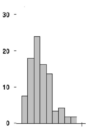
Figure 2. Example of experimental data with non-zero skewness (gravitropic response of wheat

coleoptiles, 1,790)

Consider the distribution on the figure. The bars on the right side of the distribution taper

differently than the bars on the left side. These tapering sides are called tails, and they provide a

visual means for determining which of the two kinds of skewness a distribution has:

 negative skew: The left tail is longer; the mass of the distribution is concentrated on the right of the figure. It has relatively few low values. The distribution is said to be

left-skewed. Example (observations): 1, 1000, 1001, 1002, 1003.

 positive skew: The right tail is longer; the mass of the distribution is concentrated on the left of the figure. It has relatively few high values. The distribution is said to be

right-skewed. Example (observations): 1, 2, 3, 4, 100.

If there is zero skewness (i.e., the distribution is symmetric) then the 𝑚𝑒𝑎𝑛 = 𝑚𝑒𝑑𝑖𝑎𝑛.

(if, in addition, the distribution is unimodal, then the 𝒎𝒆𝒂𝒏 = 𝒎𝒆𝒅𝒊𝒂𝒏 = 𝒎𝒐𝒅𝒆).

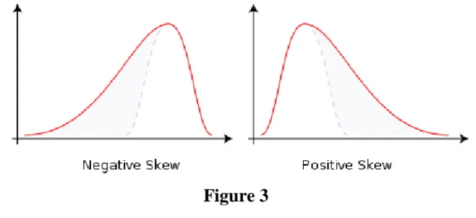
Many textbooks teach a rule of thumb stating that the mean is right of the median under

right skew, and left of the median under left skew. This rule fails with surprising frequency. It

heavy. Most commonly, though, the rule fails in discrete distributions where the areas to the left

and right of the median are not equal. Such distributions not only contradict the textbook

relationship between mean, median, and skew, they also contradict the textbook interpretation of

the median.

Figure 3

Definition

The skewness or the third standardized moment of a random variable 𝑋, is denoted 𝛾₁

and defined as

𝛾₁ = 𝜇3

𝜎3 =

𝐸 𝑋−𝜇 3

𝐸 𝑋−𝜇 23 2,

where 𝜇₃ is the third moment about the mean 𝜇, and 𝜎 is the standard deviation. Equivalently,

skewness can be defined as the ratio of the third cumulant 𝜅₃ and the third power of the square

root of the second cumulant 𝜅2:

𝛾₁ = 𝜅3

𝜅₂3 2.

The skewness of a random variable 𝑋 is sometimes denoted Skew[𝑋].

For a sample of 𝑛 values the sample skewness is

𝑔₁ = 𝑚3

𝑚₂3 2 =

1

𝑛 𝑛𝑖=1 𝑥𝑖−𝑥 3 1

𝑛 𝑛𝑖=1 𝑥𝑖−𝑥 2 3 2,

where 𝑥_𝑖 is the 𝑖𝑡𝑕 value, 𝑥 is the sample mean, 𝑚₃ is the sample third central moment, and 𝑚₂

is the sample variance.

If 𝑌 is the sum of 𝑛 independent random variables, all with the same distribution as 𝑋,

4.3 Kurtosis

In probability theory and statistics, kurtosis (from the Greek word κσρτός, kyrtos or

kurtos, meaning bulging) is a measure of the "peakedness" of the probability distribution of a

real-valued random variable. Higher kurtosis means more of the variance is the result of

infrequent extreme deviations, as opposed to frequent modestly sized deviations.

The fourth standardized moment is defined as

𝜇4

𝜎4,

where 𝜇4 is the fourth moment about the mean and 𝜎 is the standard deviation. This is sometimes

used as the definition of kurtosis in older works, but is not the definition used here.

Kurtosis is more commonly defined as the fourth cumulant divided by the square of the

second cumulant, which is equal to the fourth moment around the mean divided by the square of

the variance of the probability distribution minus 3,

𝛾₂ = 𝜅4

𝜅₂2 =

𝜇4

𝜎4− 3,

which is also known as excess kurtosis. The "minus 3" at the end of this formula is often

explained as a correction to make the kurtosis of the normal distribution equal to zero. Another

reason can be seen by looking at the formula for the kurtosis of the sum of random variables.

Because of the use of the cumulant, if 𝑌 is the sum of 𝑛 independent random variables, all with

the same distribution as 𝑋, then Kurt[𝑌] = Kurt[𝑋]/𝑛, while the formula would be more

complicated if kurtosis were defined as 𝜇_𝜎4

4.

More generally, if 𝑋₁, ..., 𝑋_𝑛 are independent random variables all having the same

variance, then

Kurt 𝑛𝑖=1𝑋𝑖 =_𝑛12 𝑛𝑖=1Kurt 𝑋𝑖 ,

whereas this identity would not hold if the definition did not include the subtraction of 3.

The fourth standardized moment must be at least 1, so the excess kurtosis must be −2 or

more (the lower bound is realized by the Bernoulli distribution with 𝑝 = ½, or "coin toss"); there

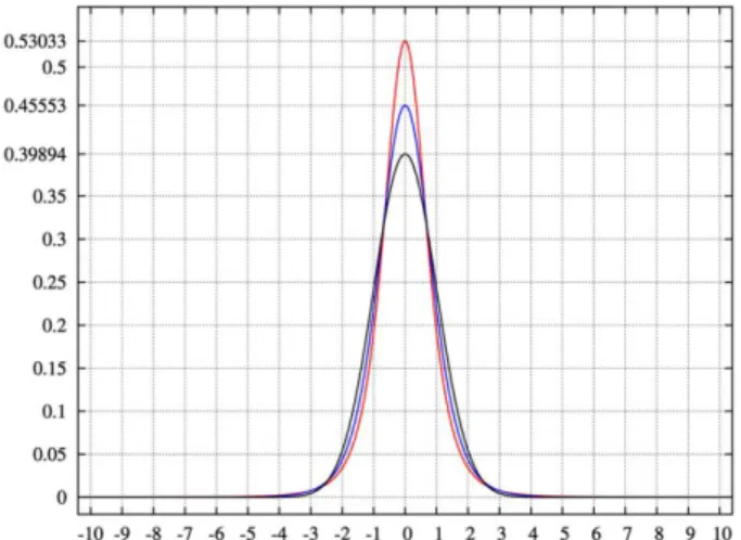
Figure 4.pdf for the Pearson type VII distribution with kurtosis of infinity (red); 2 (blue); and 0

(black)

Figure 5. Kurtosis of well-known distributions

In this example we compare several well-known distributions from different parametric

families. All densities considered here are unimodal and symmetric. Each has a mean and

skewness of zero. Parameters were chosen to result in a variance of unity in each case.

D: Laplace distribution, a.k.a. double exponential distribution, red curve, excess kurtosis

= 3

S: hyperbolic secant distribution, orange curve, excess kurtosis = 2

L: logistic distribution, green curve, excess kurtosis = 1.2

N: normal distribution, black curve, excess kurtosis = 0

C: raised cosine distribution, cyan curve, excess kurtosis = −0.593762...

W: Wigner semicircle distribution, blue curve, excess kurtosis = −1

U: uniform distribution, magenta curve, excess kurtosis = −1.2.

Note that in these cases the platykurtic densities have bounded support, whereas the

There exist platykurtic densities with infinite support, e.g., exponential power

distributions with sufficiently large shape parameter b, and there exist leptokurtic densities with

finite support, e.g., a distribution that is uniform between −3 and −0.3, between −0.3 and 0.3, and