Wang_unc_0153D_19354.pdf

T

I

G

C

M

C

, D

,

L

O

Ray Wang

A dissertation submitted to the faculty of the University of North Carolina at Chapel Hill in par-tial fulfillment of the requirements for the degree of Doctor of Philosophy in the Department of

Economics.

Chapel Hill 2020

Approved by:

Luca Flabbi

Donna Gilleskie

Andr´es Hincapi´e

Fei Li

c

2020 Ray Wang

ABSTRACT

Ray Wang: The Impact of Grades on College Major Choice, Dropout, and Labor Outcomes. (Under the direction of Luca Flabbi)

I develop a dynamic model of education and labor supply decisions that seeks to explain student

demand elasiticities to the grading standards in their courses, and the high rate of dropout from

STEM majors. The positive correlation in the data between wages and terminal GPA suggests

that firms offer a wage premium to students with higher grades, even after controlling for major.

College students consider these returns to grades when making education decisions: dropout or

major switching can be induced by grade shocks. I estimate a structural model using the NLSY97,

and find that a difference in grades by 1.0 GPA points can impact the net present value of a college

degree by as much as 20 percent at the time of graduation. If STEM and non-STEM course

grading standards were adjusted to be in line with each other, there would be a 4.7 percent increase

in the total number of STEM major graduates, a comparable effect to a $2,200 STEM tuition

subsidy. Finally, a key observation of the model is that due to imperfect sorting across majors and

occupations, large changes in the number of STEM degrees translate into smaller changes in the

ACKNOWLEDGMENTS

There are many people I must thank for their invaluable help in the dissertation process, and in

obtaining a Ph.D. in general.

First, I would like to thank my parents for supporting me and my pursuits. My Ph.D. is a

culmination of three decades of sacrifice, support, and patience on their parts, and I would not

be the person I am today without them. I would also like to thank my extended family for their

encouragement and support. I hope to make you proud.

I must also thank my advisor, Luca Flabbi, for his guidance and feedback during the

disserta-tion process. He had a major role in coalescing my unfocused research interests around my final

dissertation topic. Looking back, I can see how he helped steer me around various pitfalls, and

directed my work towards the most promising areas. His guidance has left an indelible mark on

my dissertation.

The rest of my dissertation committee - Donna Gilleskie, Andr´es Hincapi´e, Fei Li, and Ted

To - also had a key role in my research. They read various early drafts of my research, listened to

countless presentations, and took many hours of their time to offer advice and feedback. The major

improvements that my job market paper underwent, especially over the past year, are entirely due

to the helpful input of everyone on my committee.

I would also like to thank my fellow graduate students, both within the economics program

and without, for their support, feedback, and encouragement. The participants in the applied

mi-croeconomics seminar provided lots of helpful feedback and comments that helped my paper and

presentation immensely. While I cannot thank everyone by name (and for that I apologize), I would

like to express my gratitude in particular to Serge Severenchuk, Serge Korepin, and David Leather.

The two Serge’s have been excellent to me, inviting me to social events, training together, and just

making my time in graduate school much more enjoyable. David has been very supportive and

that was going through the same things I was. Thank you all for your friendship.

I would like to thank everyone at Chapel Hill Gracie Jiu Jitsu and the Carolina Judo Club.

While I may not have done much research on the mats, my time training was time well spent.

Martial arts provided me with a much needed change of pace from graduate research, and helped

me grow as a person. One of the most important lessons I learned was that while careful analysis

certainly has value, there are times when it is best to commit to decisive action. I am particularly

grateful for the patience and guidance of my many instructors: Mazi Heydary, Tim Hufford, Eric

Anderson, Nick Palmisciano, Shawn Madden, and Bill Cabrera.

Lastly, I would like to express my appreciation to everyone else who provided mentorship,

inspiration, and shared in my victories and my defeats. There are far too many to name, but I

would like to acknowledge Teymoor A., Hirohiko A., Kevin K., Aleksandar M., Jacques P., Arya

TABLE OF CONTENTS

LIST OF TABLES . . . ix

LIST OF FIGURES . . . xi

1 The Impact of Grades on College Major Choice, Dropout, and Labor Outcomes . . 1

1.1 Introduction . . . 1

1.2 Data . . . 6

1.2.1 Data Construction . . . 6

1.2.2 Data Descriptives . . . 8

1.3 Model . . . 11

1.3.1 Overview . . . 11

1.3.2 Agent Endowments . . . 12

1.3.3 Labor Market Sector . . . 12

1.3.4 Educational Sector . . . 16

1.3.5 Agent Problem and Model Summary . . . 19

1.4 Identification . . . 21

1.5 Estimation . . . 22

1.5.1 Overview . . . 22

1.5.2 The E-M Algorithm and Sequential Estimation . . . 23

1.6 Estimation Results and Discussion . . . 25

1.6.1 Labor Market . . . 25

1.7 Counterfactual Experiments . . . 45

1.7.1 Changes in the STEM Return on the Labor Market . . . 46

1.7.2 Changing Grading Policies and Major-Specific Subsidies . . . 47

1.8 Conclusion . . . 50

A Appendix . . . 52

A.1 Tables and Figures Appendix . . . 52

A.2 Data Appendix . . . 53

A.2.1 Labor Market Sector Data Construction . . . 54

A.2.2 Educational Sector Data Construction . . . 57

A.2.3 Educational Sector Structural Restrictions . . . 60

A.3 Likelihood Expression and Simulation . . . 64

A.3.1 Ex-Ante Value Function . . . 64

A.3.2 Individual Likelihood . . . 65

A.3.3 Likelihood Simulation . . . 71

A.4 Bootstrap Procedure . . . 72

LIST OF TABLES

1.1 Observed Log-Wage Regression Results . . . 9

1.2 Average SAT/HS GPA and Grade Outcomes, by Major Choice and Year in School . 10 1.3 Labor Market Characteristics by Occupational Sector . . . 10

1.4 Skilled Labor Market Parameter Estimates by Occupational Sector . . . 26

1.5 Unskilled Labor Market Parameter Estimates by Dropout Year . . . 27

1.6 Yearly Occupational Transition Matrix for College Graduates . . . 29

1.7 Yearly Employment Transition Matrix for College Dropouts . . . 30

1.8 Occupational Choice Probabilities for College Graduates, by Years Since Graduation 30 1.9 Occupational Choice Probabilities for All Dropouts, by Time . . . 31

1.10 Relative Net Present Values of Graduation or Dropout by Agent Type, Major, GPA, and College Quality . . . 37

1.11 Estimated Education Parameters, by Major . . . 39

1.12 Graduation Rate by University Type . . . 41

1.13 Choice Probabilities Among Students Still in College . . . 41

1.14 Average SAT/HS GPA and Grade Outcomes of Students, by Major Choice and Time 42 1.15 Average Grade Outcome by Current Period Decision and Next Period Decision . . 42

1.16 Average Grade in First Year, by Major Choice and Eventual College Outcome . . . 43

1.17 Mean Model-Generated Grade Shock andt+ 1Choice . . . 44

1.18 Effect of a 0.10 Log-Wage STEM Major Return Increase on Education and Labor Outcomes . . . 46

1.19 Effects of Changes in Grading Policies on Education and Labor Outcomes . . . 49

A.1 Major Classifications . . . 52

A.3 Occupational Classifications . . . 53

A.4 Characteristics of Students, by Highest Degree Obtained . . . 56

A.5 Average Yearly Earnings Within Three Years of Bachelor’s, by Highest Degree and Major . . . 57

A.6 Mapping Between NLSY97 Numeric Grades and Values Used in Paper . . . 59

A.7 Estimation Sample Construction and Mean Covariates . . . 62

A.8 Total Years of Schooling for Male College Graduates with Transcripts in NLSY97 . 63

A.9 Yearly Labor Choice Transition Matrix for College Graduates, Out-Sample . . . . 73

LIST OF FIGURES

1.1 Wage Profile for College Graduates, by Major and GPA . . . 32

1.2 Wage Profile for College Graduates, by Major and Occupational Sector . . . 32

1.3 Wage Profile for College Dropouts, by Year of Dropout . . . 33

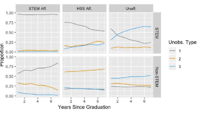
1.4 Type Distribution of Workers Over Time, by Occupational Choice and Major . . . 34

A.1 Wage Profile for College Graduates, by Terminal Major, GPA, and Occupational Sector . . . 54

A.2 Wage Profile for College Graduates, by Terminal GPA and Occupational Sector . . 55

A.3 Wage Profile for Out-Sample, by Major and GPA . . . 75

A.4 Wage Profile for Out-Sample, by Major and Occupational Sector . . . 75

CHAPTER 1

THE IMPACT OF GRADES ON COLLEGE MAJOR CHOICE, DROPOUT, AND LABOR OUTCOMES

1.1 Introduction

A key policy concern in US higher education is the high rate of attrition from college, as well as

the high rate of attrition from STEM majors (Science, Technology, Engineering, and Mathematics).

Only 60 percent of students who started a bachelor’s program in 2008 obtained a degree by 2014,

and only half of the students who started out interested in STEM courses1 _{persisted through their}

sophomore year, instead switching majors or dropping out entirely (Griffith, 2010).2 _{STEM majors}

made up only 18 percent of all bachelor’s degrees awarded in the US in 2016 (NCES, 2019).

This behavior occurs despite the large differences in earnings between STEM majors, non-STEM

majors, and college dropouts: median lifetime earnings in the US are $1.44 million for mathematics

and statistics majors, $0.99 million for English majors, and $0.72 million for college dropouts

(2014 dollars) (Hamilton Project, 2014).3 Policymakers seeking to increase the number of STEM

workers must first understand the underlying mechanism that drives the proportionally low number

of STEM majors.4

What explains the high rate of attrition from STEM majors, and their overall low

representa-tion? One possibility is the grades a student receives in college have an impact on their earnings

post-graduation. The correlation between grades and earnings is well-documented in the literature,

1_{‘Interest in STEM’ defined as students directly stating an interest in majoring in STEM, or taking at least half of}

their first-year courses in STEM.

2_{There is no significant compensating transition of non-STEM majors to STEM majors: less than 15 percent of}

students initially interested in non-STEM eventually graduate with a STEM degree.

3_{Values are from the American Community Survey, a representative sample of US workers conducted by the US}

Census Bureau.

4_{For example, in 2012 the President’s Council of Advisors in Science and Technology stated a need for one million}

with wage regressions estimating a 6-10 percent return to yearly earnings per GPA point (Finnie

et al., 2016; Jones and Jackson, 1990).5 Furthermore, at Duke University, average grades in STEM

courses were lower than those in other majors by ∼ 0.3GPA points, despite students in STEM majors having higher average SAT scores (Arcidiacono et al., 2012). These grading differences

between STEM and non-STEM majors are also observed at other universities such as Princeton

University, Wellesley College, and the University of Michigan (Princeton ODC, 2017; Butcher

et al. 2014; Achen and Courant 2009). Thus, students choosing between STEM and non-STEM

majors may be considering the monetary payoffs both to major, and also to the grades that they

expect to receive in that major.

Perhaps the strongest evidence that students care about grading standards is their responses to

university grade deflation policies. Grade deflation policies are meant to counteract grade

infla-tion, the upward trend in historical grades awarded to students: in 1960, the average grade among

all universities in the US was a 2.4; by 2013, the average was over 3.1 (Rojstaczer and Healy,

2010; Rojstaczer, 2016). Given that grades are a useful source of information both to students

and employers, administrators at universities such as Wellesley and Princeton implemented grade

deflation policies: Wellesley placed a cap on the average grade at introductory courses at a 3.33;

Princeton aimed to have at most 35 percent of grades awarded by each department be A’s or A-’s

(Butcher et al. 2014; Princeton Ad Hoc Comm., 2014).6 These policies did not affect all

depart-ments equally: STEM departdepart-ments were generally already ‘in compliance’, and the affected (i.e.

the ‘policy-treated’) courses or majors were primarily in the humanities and social sciences,

ex-cluding economics. Student response to these policies was strongly negative: ‘treated’ departments

at Wellesley saw a reduction in majors by 30 percent (∼ 8students), and 59 percent of Princeton students surveyed in 2014 reported a ‘negative’ or ‘strong negative’ impact of the grade deflation

policy on their college experience.

5_{The earnings differences between graduates with high and low GPAs, controlling for field of study, do not}

signif-icantly widen or shrink over the life cycle.

6_{These guidelines allowed for instructor discretion in grading, but in practice were effective in achieving their}

To rationalize this strong student response to grades, I propose a dynamic model of educational

and occupational choice where grades show up directly in the expected productivity of workers,

from the perspective of firms. There is evidence that employers use unweighted GPA as one of

the summary statistics of a student’s academic performance (Princeton Ad Hoc Comm., 2014),

and that employers are less likely to interview or hire applicants with low GPAs (Koeppel, 2006;

Piopiunik et al., 2018). There is also evidence that higher grades translate directly into wages:

Khoo and Ost (2018) find that Latin honors, which are awarded for a GPA above a certain numeric

cutoff, command a wage premium. In my model, I allow for a linear log-wage premium associated

with grades and assume that it is constant over experience7; students thus care about the levels of

their grades while in college, since these grades will directly affect lifetime earnings. I am agnostic

about the foundations of the returns to grades (e.g. it may result from employers using grades as

a signal of productivity) and do not explicitly model their origin, although the structure of wage

dynamics that I use is broadly consistent with other findings in the literature, such as Arcidiacono

et al. (2010), which I will discuss in further detail in the model specification section.

My model, based on the dynamic occupational choice framework of Keane and Wolpin (1997),

adds grades to the wage equation for college graduates, and imposes additional structure to the

educational sector. Each year, college students have the option to continue their education by

choosing to focus on STEM or non-STEM, or to drop out. In addition to the preference and wage

shocks standard to these types of dynamic structural models (e.g., Sullivan 2010), students are also

subject to grade shocks: while they know what the distribution of their potential grades is, they

are uncertain about their realized grade. Negative grade shocks can affect a student’s future labor

market earnings, reducing their expected discounted value of graduating and causing them to drop

out instead of trying to graduate with a low GPA. Once students finish their education, they enter

the labor market. I allow the returns to major and grade to vary by occupational sector, since the

literature has found that working in an occupation related to one’s major commands a significant

wage premium (Kinsler and Pavan, 2015; Robst, 2007), and because not all STEM majors work

in STEM occupations, and vice versa. By taking a structural approach, I am also able to account

for unobserved agent heterogeneity in nonpecuniary preferences for occupation and major, as well

as academic ability and labor market productivity, two factors which complicate estimation of the

wage returns to major via reduced-form methods such as instrumental variables (Altonji et al.,

2016). By modeling the decisions of agents through college and into the labor force, I endogenize

the relationship between major and occupation, and am able to distinguish between graduating

with a degree in STEM versus actually working in STEM occupations.

I estimate my model using the National Longitudinal Survey of Youth (1997), which contains

data on both educational decisions (major choice and dropout) and outcomes (grades), as well

as occupational decisions (occupational sector/hours worked) and outcomes (wages). Having

in-formation both pre- and post-graduation is critical to accounting for the selection processes into

major as well as occupation, and allows for structural identification of parameters such as the

re-turns to major and GPA. While I estimate the model using simulated maximum likelihood, I reduce

the computational burden of the estimation by using the sequential E-M algorithm, as outlined in

Arcidiacono and Jones (2003). By using the E-M algorithm, I am able to sequentially estimate

the labor market parameters and then the educational sector parameters while still allowing for

unobserved heterogeneity.

I estimate significant returns to major as well as grades, which vary by occupational sector: in

STEM affiliated occupations, a STEM major (with average grades) commands a 0.29 premium in

log-wages over a non-STEM major; however, for humanities and social-science affiliated

occupa-tions, a non-STEM major has a 0.24 log-wage premium over STEM. I find the returns to grades

are significantly larger when the major and occupation ‘match’: a 1.0 increase in GPA for STEM

majors in STEM occupations corresponds to an increase in log-wages by 0.20, whereas a 1.0

GPA increase for non-STEM majors in humanities and social-science affiliated occupations only

increases log-wages by 0.003 (the converse, at a smaller magnitude, is also true for non-STEM).

Using my estimated parameters, I conduct a series of counterfactual experiments. First, I

look at the impact of an increase in the wage returns to STEM majors, to assess the elasticity

in the literature that STEM courses are graded more stringently than non-STEM courses, I conduct

a series of grading policy counterfactuals, that either deflate non-STEM grades, inflate STEM

grades, or a combination of both. I find that a grading policy that adjusts both STEM grades and

non-STEM grades so that they align (while the grade premium on wages stays constant) increases

the total number of STEM graduates by 4.7 percent relative to baseline, a comparable effect to a

major-specific tuition policy that subsidizes STEM majors by $2,200 yearly and increases tuition

by $660 yearly for non-STEM majors.

Importantly, I find in all of these counterfactuals that the relative increases in STEM major

choice significantly exceed the relative increases in STEM occupation choice: for example, while

the counterfactual grade policy discussed above increased the number of STEM majors by 4.7

percent, the number of STEM workers nine years out increased only by 3.9 percent. The distinction

between STEM majors and STEM workers – which is often glossed over in research that focuses

only on major choice – is an important one, since many educational policies are ultimately more

concerned with the latter rather than the former. For example, while the President’s Council of

Advisors on Science and Technology (2012) cites a ‘need to add to the Americanworkforceover

the next decade approximately 1 million more STEM professionals’, the recommendations are

focused on adding ‘an additional 1 millionSTEM degrees’ (italics mine).

While there is a large literature on major choice and college dropout, most have as their central

mechanism students learning about their own ability over time and making dynamic decisions

as their uncertainty is resolved (Arcidiacono, 2004; Arcidiacono et al., 2016; Stinebrickner and

Stinebrickner, 2013; Stange, 2012). Instead, in my model, students have no uncertainty about their

own ability, only about the grade, preference, and wage shocks in the model. One key difference

of this paper from the existing literature is that, to the best of my knowledge, it is the first to

structurally assess the importance of grading standards themselves on students’ decisions over

major or dropout; grading standards remain fixed in counterfactual analyses in the other papers.

The rest of the paper is organized as follows. Section 2 describes the data as well as the main

stylized moments that motivate the model. Section 3 describes the model. Section 4 discusses

estimation results as well as model goodness of fit along a number of dimensions associated with

student selection, sorting, and dropout while in college. Section 7 contains the results of a series

of counterfactual experiments, including grading policy changes. Section 8 concludes.

1.2 Data

1.2.1 Data Construction

I use the National Longitudinal Survey of Youth, 1997 (NLSY97), coupled with Geocode data,

for estimation. The NLSY97 is a nationally representative sample of 8,984 youths between the

ages of 12 and 16 as of December 31, 1996. The first interview was conducted in 1997, with

annual follow-up interviews until 2011, and biannual interviews afterwards (2013, 2015). Since my

model involves yearly decisions, I only use the data up until 2011. I restrict the estimation sample

to men who attended at least one year of a 4-year college and who have college transcript data

from the Post-Secondary Transcript Study (PSTRAN) part of the NLSY97; the PSTRAN provides

information on a student’s courses taken while in college, as well as the grades he received. I

further restrict the data to students who can be represented as potentially graduating in four years

(if they do not drop out); this sample restriction means that among college graduates, I only include

those who finish in four years or who have four years where they take at least six courses that year,

so that I ‘drop’ the year where they take fewer than six courses. This restriction is primarily

for tractability: modeling an intensive margin of course credits or allowing heterogeneity in the

number of years to graduate would make the model much more complex.8 My final estimation

sample consists of 2,887 observations for 306 men. Details about sample construction and data

classification and cleaning are available in the Data Appendix.

The NLSY97 data contain information on SAT scores and high school GPA, college transcripts

for students in college, and occupational sector and annual wages for students in the labor force.

The Geocode supplement to the NLSY97 provides an IPEDS identifier that allows me to

deter-mine the identity of the college the student attended. I use the 2001 U.S. News & World Report

Best Colleges rankings of universities to classify universities as elite or non-elite, depending on

if they were in the top 50 or not. The IPEDS also reports whether the university is public,

pri-vate religious, pripri-vate non-religious, or for-profit. Lastly, to determine yearly education costs, I

use historical university-published tuition values as collected by Chronicle of Higher Education

(2018), subtracted by the student’s self-reported scholarships, deflated to 1996 dollars using the

BLS ‘College tuition and fees’ index.9

I classify a student as majoring in STEM in a given year if at least half of the courses he

takes are in STEM departments; my classification of STEM majors is given in Table A.1, and

is similar to Arcidiacono et al. (2016). Roughly, ‘STEM’ means natural sciences, engineering,

mathematics. Grades are calculated by taking the average of the reported numeric term grades in

each academic year, or if not reported, by taking an average of grades over all courses taken that

year. I take the student’s highest reported SAT scores, or use their predicted SAT scores given their

Armed Services Vocational Aptitude Battery (CAT-ASVAB) scores, if those are missing; I do not

distinguish between the two measures in estimation. The linear regression that I use to predict SAT

scores is given in Table A.2.

I classify a student as working if he worked on average 20 hours a week for that year, and for

college graduates, I assign him to one of three occupational sectors – STEM affiliated, humanities

and social science (HSS) affiliated, and unaffiliated – using his 2002 Census Occupational

Cate-gory; the mapping is given in Table A.3. I define the three occupation categories based on whether

the occupations directly relate to a student’s coursework and education in the corresponding

ma-jors: ‘STEM affiliated occupations’ are those that require skills directly obtained in a ‘Science,

Technology, Engineering, and Mathematics’ major (e.g., engineers); ‘HSS affiliated occupations’

as those that require coursework in humanities and social sciences (e.g., teachers); and

‘unaffili-ated occupations’ are those that do not clearly require coursework in a particular major, and largely

include ‘blue’ and ‘pink’ collar occupations (e.g. salespeople).10 All working college dropouts are

9_{I assume all students at a public school are charged the in-state tuition value. While students self-report tuition}

values in the NLSY97, I find the data to be unreliable, as a majority of my sample reported receiving financial aid exceeding their reported tuition.

10_{In other words, if a job posting for a typical job in a given occupation requires a student have a bachelor’s degree}

classified as working in a single unskilled sector. Hourly earnings are calculated by taking

re-ported yearly income and weekly hours worked for the year, scaled to an equivalent of 2087 hours

worked over 52 weeks11, and deflated to 1996 dollars.12 I do not consider advanced degrees in

my estimation, so I drop observations for individuals once they start working towards their PhD

or professional degree (DDS, JD, MD), and afterwards. I do not find consistent jumps in earnings

for individuals who obtain a masters degree, across all three occupation types, so I ignore

mas-ters degrees in my wage equation specification and do not drop those observations. Furthermore,

while there is evidence that students that pursue PhDs or professional degrees are stronger

academ-ically, they actually earn less in their first jobs out of college than students that do not eventually

pursue advanced degrees (see Tables A.4 and A.5 and the accompanying discussion in the Data

Appendix), suggesting that my final estimates may actually understate the returns to grades.

Lastly, in the data there are a large number of individuals who have missing data for their

edu-cation outcomes, but that eventually obtain a bachelor’s degree and have labor market observations

(848 observations over 184 men). Since these individuals are observably different from the

indi-viduals for whom I have complete educational and labor data, in particular in the percentage of

them obtaining a STEM degree, I do not use them in my main estimation of the model. However,

I do use these individuals as a part of an out of sample evaluation of goodness of fit of my labor

market parameter estimates.

1.2.2 Data Descriptives

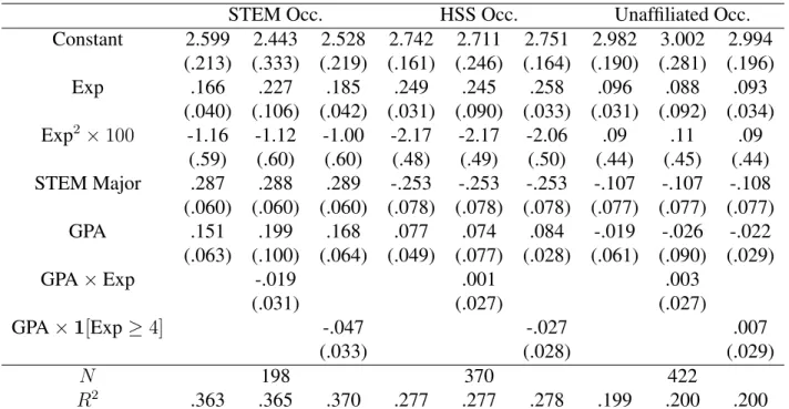
Table 1.1 shows the results of a series of simple wage regressions, split by skilled occupational

sector, controlling for own-sector experience and major, and varying in the form of dependency

on grades. There is a positive and significant coefficient on grades for STEM occupations, a

positive but insignificant coefficient for HSS, and a small and insignificant negative coefficient for

unaffilated, across all three specifications. Notably, when I include the interaction of GPA and

11_{The 2087 yearly hours value is derived from the US Office of Personnel Management.}

12_{The NLSY97 has automatically-calculated hourly wages, but I found these numbers to be unreliable, e.g. with}

Table 1.1: Observed Log-Wage Regression Results

STEM Occ. HSS Occ. Unaffiliated Occ.

Constant 2.599 2.443 2.528 2.742 2.711 2.751 2.982 3.002 2.994

(.213) (.333) (.219) (.161) (.246) (.164) (.190) (.281) (.196)

Exp .166 .227 .185 .249 .245 .258 .096 .088 .093

(.040) (.106) (.042) (.031) (.090) (.033) (.031) (.092) (.034)

Exp2×100 -1.16 -1.12 -1.00 -2.17 -2.17 -2.06 .09 .11 .09

(.59) (.60) (.60) (.48) (.49) (.50) (.44) (.45) (.44)

STEM Major .287 .288 .289 -.253 -.253 -.253 -.107 -.107 -.108

(.060) (.060) (.060) (.078) (.078) (.078) (.077) (.077) (.077)

GPA .151 .199 .168 .077 .074 .084 -.019 -.026 -.022

(.063) (.100) (.064) (.049) (.077) (.028) (.061) (.090) (.029)

GPA×Exp -.019 .001 .003

(.031) (.027) (.027)

GPA×1[Exp≥4] -.047 -.027 .007

(.033) (.028) (.029)

N 198 370 422

R2 _{.363 .365 .370 .277 .277 .278 .199 .200 .200}

Note: Coefficients are for yearly log-earnings, in thousands. Exp. is own-sector experience, not counting other-sector experience, and is measured in years.

experience, I find the coefficient to be very small relative to GPA and insignificant; this finding

suggests that the ‘returns’ to GPA are constant over the experience profile. Lastly, the differences

in the coefficients on majoring in STEM suggest that the return to STEM is heterogeneous in

occupation.

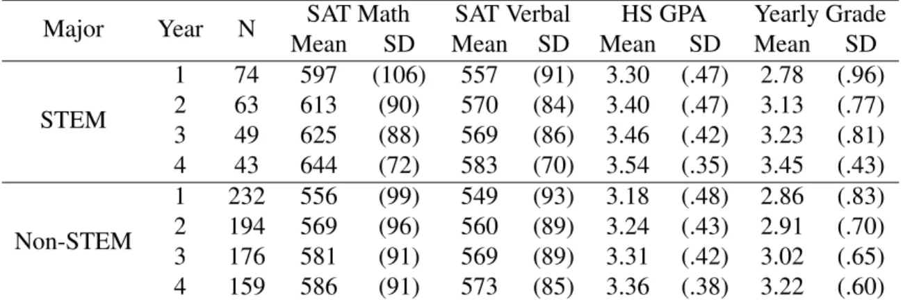
Looking at the characteristics of students who persist in college (Table 1.2), we see that high

school measures of academic ability (SAT scores and high school GPA) and realized college grades

are increasing with tenure for persisters. While the positive trend in high school ability, which

is ‘pre-determined’ prior to college, suggests that students who drop out are less academically

prepared than those who persist, interpreting the increase in realized college grades as evidence of

positive selection on academic ability is complicated by the fact that grading standards may change

by year: courses taken by a student in their fourth year of college may be graded more leniently

than those in their first year. Lastly, there is also evidence of sorting by major: students majoring

Table 1.2: Average SAT/HS GPA and Grade Outcomes, by Major Choice and Year in School

Major Year N SAT Math SAT Verbal HS GPA Yearly Grade

Mean SD Mean SD Mean SD Mean SD

STEM

1 74 597 (106) 557 (91) 3.30 (.47) 2.78 (.96)

2 63 613 (90) 570 (84) 3.40 (.47) 3.13 (.77)

3 49 625 (88) 569 (86) 3.46 (.42) 3.23 (.81)

4 43 644 (72) 583 (70) 3.54 (.35) 3.45 (.43)

Non-STEM

1 232 556 (99) 549 (93) 3.18 (.48) 2.86 (.83)

2 194 569 (96) 560 (89) 3.24 (.43) 2.91 (.70)

3 176 581 (91) 569 (89) 3.31 (.42) 3.02 (.65)

4 159 586 (91) 573 (85) 3.36 (.38) 3.22 (.60)

Note: Yearly grade is the grade received for that year, not cumulative GPA.

Table 1.3: Labor Market Characteristics by Occupational Sector

Occupational Sector: STEM HSS Unaffiliated

Mean SD Mean SD Mean SD

% Workers with STEM Major 62.8 (3.4) 9.6 (1.5) 10.5 (1.5)

Ann. Log-Earnings, STEM Major 3.58 (.35) 3.01 (.39) 2.63 (.41)

Ann. Log-Earnings, Non-STEM Major 2.66 (.46) 3.06 (.55) 2.95 (.57)

N 207 387 445

Note: Annual log-earnings are in thousands of dollars, and are for observed wages 2 years after graduation (there are a large proportion of choices in home production in the first year).

Table 1.3 presents some summary characteristics of workers in each occupational sector.

Re-garding the mapping between major and occupation, there is mixing: some non-STEM majors

work in STEM occupations, and vice versa. Furthermore, although a STEM major earns log-wages

that are on average 0.57 higher in STEM occupations than HSS occupations (and even higher

rel-ative to unaffiliated occupations), approximately 10 percent of the workers in the non-STEM and

unaffiliated sectors have STEM degrees. The reverse is also true for workers in STEM occupations

but with degrees in non-STEM. This statistic suggests the presence of nonpecuniary preferences

for occupation, since the variation in occupational choice is not fully explained by variation in

wages.

My model explains two stylized facts: college GPA is positively correlated with labor market

earnings, and students who persist in college are progressively stronger in pre-college

I include nonpecuniary preferences for occupation in my model; this feature will prove important

when measuring the ‘pass-through’ rate of changes in numbers of STEM majors to changes in

STEM workers, as well as accounting for selection into major and occupation. My model also

replicates a number of other moments of the data, such as the general wage profile and choice

patterns of education and occupation. Finally, when considering policy experiments, I show that

my counterfactual results replicate the negative student choice response to grade deflation policies,

as observed in the literature.

1.3 Model

1.3.1 Overview

I now describe the key characteristics of the model. After graduating from high school and

being accepted to a particular university, agents make yearly decisions over education or labor

alternatives. For those students who have not yet dropped out or graduated, they can either take

courses in STEM or non-STEM majors (subject to a few choice restrictions to be outlined later), or

choose to drop out of college and engage in either unskilled labor or home production. Dropping

out of college is absorbing: there is no re-entry. For agents who have dropped out of college, they

receive wage offers from a single unskilled labor sector, and can choose to work or engage in home

production. For agents who successfully graduate from college, they receive three wage offers from

the three types of skilled occupational sectors (STEM affiliated, HSS affiliated, and unaffiliated),

and can choose to work in any one of the three sectors, or engage in home production. There

is complete labor market separation between graduates and dropouts: graduates do not have the

option to work in the unskilled sector, and dropouts do not have the option to work in any of the

skilled sectors. There is no option for graduate school or further education, and agents have a finite

horizon decision problem ending at some terminal retirement age.

Agents are forward-looking and choose a sequence of actions that yields the highest expected

lifetime utility. Per-period utility derives from wages as well as a flow utility for each

alterna-tive (psychic/nonpecuniary cost or consumption value of working/education). Agents are

uncer-tain over grade shocks, wage shocks, and preference shocks; however, they know perfectly their

perfectly the structural parameters that dictate the grade generating process as well as wage offer

process (i.e. technology).

1.3.2 Agent Endowments

Agents are heterogeneous in both observed and unobserved (to the researcher) dimensions.

Observed characteristics for agent iare denoted by the vector XHS

i and include the agent’s SAT

Math and Verbal scores, as well as their high school GPA. In the style of Heckman and Singer

(1984), I also use a finite mixture approach for agent-specific unobserved heterogeneity: agents

are one of three researcher-unobserved types, and these types differ in the dimensions of academic

ability and preferences, and productivity and preferences by occupational sector. Agents know

their type perfectly. Denote the three types by{θ1, θ2, θ3}with corresponding population

propor-tions {π1, π2, π3}. I do not assume any particular form of correlation between agent observable

characteristics and unobserved type.

1.3.3 Labor Market Sector

The labor market sector consists of two broad types of sectors, the skilled and unskilled sectors,

which are completely separate. Since my dissertation is focused on the margin of major switching

among students who intend to graduate, I further divide the skilled sector into three occupational

types, while treating the unskilled sector as a single ‘occupational type’. College graduates make

their labor decisions over 30 periods following their graduation, up to a terminal period oft = 34; college dropouts can make labor decisions starting as soon as they drop out untilt= 34.13

The skilled sector consists of STEM affiliated, HSS affiliated, or unaffiliated occupational

sec-tors. A college graduate can choose to work in any of these three skilled occupational sectors

j = 1,2,3or engage in home productionj = H, regardless of his major; however, his expected productivity may differ for each sector. Within each of the occupational sectors, firms are identical:

the agent thus makes decisions over occupational sectors for each year. These sectors are

compet-itive between firms, and firms have the same information: thus firms offer the agent his expected

13_{There is no additional terminal payoff att = 34, e.g. a retirement payoff that depends on some state variables.}

productivity given the firm’s information. An agent that works in a particular sectorj receives that particular wage offer, and also accumulates one unit of experience in sectorj.

I assume that log-productivity in skilled occupational sector j can be expressed as the sum of a deterministic component of productivity that depends on the rental rate of labor in that sector,

agent endowments in that sector, a student’s terminal major and GPA, and human capital from

the vector of accumulated work experience; as well as an idiosyncratic productivity shock (i.e. a

period-specific match quality or some fleeting productivity shock that is common to the sector).

I allow all of these components to vary by occupational sector j. In particular, I assume the log-productivity of the worker from the perspective of the firm is shifted by an indicator for whether

the student’s terminal major was in STEM, and linearly with respect to their GPA, with the returns

to GPA allowed to differ by major; these returns to major and GPA do not change with work

experience (see Eqn. 1.1). This specification is consistent with the results of my reduced form

wage regression (Table 1.1) as well as other empirical findings in the literature. Finnie et al.

(2016) find that, after controlling for field of study, there is a log-wage premium for having higher

grades and the time-grade interaction term is not significantly different from zero for most fields of

study.14 Arcidiacono et al. (2010) apply an employer-learning model (i.e., the model of Altonji and

Pierret 2001) to the NLSY79 and find that while underlying productivity, as measured by AFQT

scores, is initially hidden from employers and revealed over time for high school graduates, it is

essentially revealed immediately for college graduates; empirically, this is shown by estimating

the AFQT-experience interaction term to be zero for college graduates. If grades were one useful

predictor of productivity and there was no additional employer learning after an individual starts

working, then one would expect the grade-experience interaction coefficient to be zero as well, as

in my model’s specification. That being said, my model is a partial equilibrium model that focuses

on agent responses to returns on grades and major; I do not take a stand on the precise mechanism

14_{They obtain a negative estimate of the time-grade interaction for males in engineering (significant at 5 percent}

generating the returns to grades and major.15

In the skilled sector, the agent i of type n has an expected log-productivity in sector j that depends on the skill rental rate rj₀, his type-specific skill endowment in that sectorr_endn,j, an indi-cator for university qualityQi, an indicator for whether his terminal major was in STEMMi, his

unweighted terminal GPAGi(and the interaction with his major), his vector of accumulated

expe-rience in all 3 sectors(x1

it, x2it, x3it)and an i.i.d. productivity shockWijt ∼ N(0, σ2j).16 There is no

correlation between the technology shocks across sectors or across time. The functional form of the

log-productivity is a quadratic in own-sector experience and linear in other-sector experience, with

an additional first-year experience effect. Finally, I impose a constraint that the own-experience

component of log-productivity cannot be decreasing in experience:

χn,j_it =

r₀j +r_endn,j +rj_q·Qi +r_Mj ·Mi+rj_G·Gi+rj_{M G}·(Mi×Gi)+ r₁j·x1_it+r₂j ·x2_it+rj₃·x3_it+rj_sq·(xj_it)2+r_onej ·1{xj_it >0}+W_ijt

, ifxj_it≤ − r j j 2rjsq

(1.1)

However, ifxj_it >− r

j j

2rsqj , I set the log-wage contribution from the own-sector experience

xj_itto be the maximum of the quadratic: for example, for sectorj = 1,

χn,_it1 =

r₀1+r_endn,1 +r1_q·Qi+r1M ·Mi+r1G·Gi+r1M G·(Mi ×Gi)+ r₂1·x2_it+r₃1·x3_it+r1_one·1{x1

it >0} − (r1

1)2

4r1

sq

+W_i1t

, ifx1_it >− r

1 1

2r1

sq

(1.2)

The constraint that the experience profile in own-sector cannot be decreasing is added to stabilize

the estimation procedure: the discounted future payoffs are very sensitive to the magnitude of the

quadratic term, which has poor empirical identification.17

15_{Later, when discussing specific counterfactual policies, I argue that the conclusions of my partial equilibrium}

model are likely to be close to reality even in a general equilibrium setting.

16_{The only relevant characteristic of the university itself in the labor market is its dummy for quality. I observe other}

characteristics of the university such as whether it is public/private, which are relevant in the educational decisions but not in the labor market productivity.

There is only one occupational sector available to dropouts: the unskilled sector. The agent’s

log-productivity is a non-decreasing quadratic in unskilled experiencexU_it. There is no heterogene-ity in the skill endowments by unobserved type n. Because unskilled workers by definition do not have a college degree, there is no dependency on grades, major, or college quality; however,

I do allow the log-productivity intercept and first-year experience effect to vary if the individual

dropped out or failed out at year four (y = 4) vs. earlier (y < 4).18 _{The returns to experience} outside of the first-year experience effect are constrained to be the same for all dropouts. The

log-productivity specification in the unskilled sectorU is:

χU,y_it =r₀U,y+r₁U ·xU_it+rU_sq·(x_itU)2+r_oneU ·1[x_itU,y >0] +W_{iU t}, ifxU_it ≤ −r U sq 2rU

1

(1.3)

χU,y_it =r₀U,y− (r U

1)2

4rU sq

+r_oneU ·1[xU_it >0] +W_{iU t}, ifxU_it >− r U sq 2rU

1

(1.4)

For each skilled occupational alternativej, the agent’s per-period flow utility is a linear function of his wage offerWj(sn_it)(i.e., the productivity including the shock) multiplied byγp; a nonpecu-niary psychic costγj(sn_it)which depends on his unobserved typen; his history of choices, college outcomes, and shocks up to and including timet, denoted bysn

it; and a Type I extreme value

pref-erence shockP

ijt(technicallyPijt is included insnit). The per-period utility of occupational sector

alternativej is:

uj(snit) =γ j

(sn_it) +γp·Wj(s_itn) +P_ijt, j ∈ {U,1,2,3} (1.5)

γj_(sn

it)consists of a constant termγconsn,j which depends on the occupation and agent type, but also

two additional nonpecuniary terms: an ‘entry cost’ γ_entryj that applies if the agent has no prior experience in the specific occupational sector, a ‘switching cost’ γ_switchj that applies if the agent

wage growth. According to the American Community Survey, yearly wages for full-time workers with a college degree peak and start to decrease at around 20-25 years in the workforce (Hamilton Project, 2014).

did not work in sectorj in the prior periodt−1, and a sector-specific shifterγ_{f irst}j that applies for the first year out of college (t= 5):

γ_ijtn =γj(sn_it) =γ_consn,j +γ_entryj ·1[xj_it= 0] +γ_switchj ·1[di,t−1 6=j] +γf irstj ·1[t= 5], j ∈ {1,2,3}

(1.6)

The entry cost, first year out of college, and switching costs do not vary by unobserved typen. For the unskilled sector, the functional form of the nonpecuniary flows is analogous, but

with-out the first-year with-out of college costs. I also allow the per-period flow utility and switching cost to

vary if the student dropped out/failed out in year 4 (y= 4) vs. otherwise (y <4):

γ_{iU t}y =γU,y(sn_it) =γ_consU,y +γ_entryU ·1[xU_it = 0] +γ_switchU,y ·1[di,t−1 6=U] (1.7)

Students who drop out or fail out in their fourth year differ from those that drop out earlier in

their level and first-year effect of unskilled wage offers, as well as their per-period flow utility and

nonpecuniary switching costs with unskilled labor; the other parameters are the same. There is no

heterogeneity in the unskilled labor market by typen.

Lastly, if the agent engages in home production, I assume it does not generate any income, and

I normalize the per-period flow utility from home production to zero, so that the per-period flow

utility is given by the Type I extreme value preference shock.

uH(snit) = P

iHt (1.8)

1.3.4 Educational Sector

As is apparent in the wage equations (Eqns. 1.1, 1.2), a student’s performance while in college

as well as his choice of major affects his labor market earnings. Students must therefore take

into account the impact of his uncertain educational outcomes on his later lifetime earnings when

individuals who are observed to attend at least one year of college. Thus, the quality q of the college as well as the type of college (public, private religious, private non-religious, or for-profit)

is fixed for the agent. While in college, agents have up to four alternatives: take a course load

specializing in STEM or non-STEM, or engaging in home production or working in the unskilled

labor market. The latter two options are available at any time while in college, and are considered

dropout: the student is only be able to work in the unskilled sector or engage in home production

for the rest of their lifetime if they drop out.

Agents receive a nonpecuniary flow utility from choosing STEM S or non-STEM N for that year, which varies by his unobserved typen, the type of universitys the student attends (public, private religious, private non-religious, or for-profit), the cost of tuition minus grants/scholarships

ctuit

i , and a Type I extreme value preference shock.19 I also include a switching cost for each major

for every year past the first year. The full functional form of the per-period utility is given by:

uj,s(snit) =γ n,s ijt −γ

p_·ctuit

i +Pijt, j ∈ {S, N} (1.9)

where

γ_ijtn,s =γ_consn,j +γ_switchj ·1{di,t−1 6=j andt≥2}+γs,j, j ∈ {S, N} (1.10)

γ_ijtn,s, j ∈ {S, N}can be thought of as the psychic cost/consumption benefit of attending college and specializing in majorj, which varies through the individual’s type viaγn,j

cons (the type has varying

preferences for major) and university type viaγs,j_{(majors differ in their consumption values across}

different university typess), andP

ijtis a Type I extreme value preference shock. This flow utility

does not change over the four years of college. Note that the flow utility of college does not

depend on the student’s academic ability or grades. The flow utilities for home production and the

unskilled sector are the same as in the labor market. Lastly, if the student successfully graduates

19_{School quality does not affect the nonpecuniary flow utility of college. The net cost of education is assumed to be}

from college, then they receive a one-time nonpecuniary payoffγgradat the start of the next period,

t= 5, which is the same across student typesnand university typess.

After enrolling in a major, the agent receives a single grade that represents the average of all

their grades for that year.20 In each year, after deciding to enroll in STEM or non-STEM, the agent

of type n at university of quality q receives a grade Gn,q_ijt in major j which depends on his high school characteristicsXHS

i (SAT scores and high school GPA) throughλHSj , the year and quality

of the university throughλq_j,t, his type-specific major abilityAn

j, and an idiosyncratic grade shock G_iqjt ∼N(0, σ_qjt2 )which has a variance that depends on the quality of the university, the major, and whether the student is an under- (t= 1,2) or upper-classman (t= 3,4):

Gn,q_ijt =X_iHSλHS_j +

4 X

s=1

(1{t=s} ·λq_jt) +An_j +G_iqjt, j ∈ {S, N}, t∈ {1,2,3,4} (1.11)

Thus, between elite and non-elite universities, grades in the same major have the same returns to

SAT scores and high school GPAλHS_j , but the levels of the gradesλq_jt as well as the variances of the grade shocksσ2

qjt may differ. To identify the levels of the grade parameters, I normalize the

major-specific ability termAn

j to be zero for typen = 1individuals, for both majors.

Importantly, grades are revealed after the individual chooses a major. The agent must take

expectations over their grade outcomes: he knows all of the parameters in the grade generating

process, so he can perfectly forecast his potential distribution of grades for both majors, but not

the precise outcome. These grade shocks will be a major driver of the decision to switch or drop

majors.

Lastly, I introduce a series of choice restrictions while in college which are meant to capture

some aspects of the ‘switching costs’ between majors. They are:

1. Major declaration at year 3: The student’s choice of major at timet= 4must be the same as his choice of major att= 3, unless he dropped out.

20_{In reality, students do not face a binary choice between STEM and non-STEM, but rather an intensive choice of}

2. STEM major pre-requisite: To choose STEM att = 3, the student must have chosen STEM in at least one of the two prior years,t= 1,2.

3. Deterministic graduation and failout. After four years in college, the student’s unweighted

cumulative GPAGi, the simple average of their four yearly grades, is calculated. IfGi <2.0,

the student fails out of college and can only work in the unskilled sector. Otherwise, he enters

the skilled sector in the next period with his terminal major corresponding to the major choice

att = 4, and terminal GPAGi.

As is shown in the Data Appendix, the first two restrictions are largely borne out by the data; the

largest restriction is actually the condition that students graduate within four years.

1.3.5 Agent Problem and Model Summary

To summarize, the model timing and sequential decision process is as follows:

1. Agentiof typenenters periodtwith his historysn_it.

2. Each eligible firm forms a match-specific productivity shock with the individualW

ijtand

sub-mits a wage offer. When in college or in the unskilled workforce, the agent only receives

wage offers for the unskilled sectorj =U. When in the skilled workforce, he observes wage offers for each skilled sectorj ∈ {1,2,3}. Wage offers depend on his college performance, accumulated experience, and the productivity shock. Unskilled productivity shocks are

dis-tributedN(0, σ2

U), and skilled productivity shocks are distributedN(0, σj2), j ∈ {1,2,3}.

3. Preference shocksP_ijtare also revealed for all employment and education alternatives avail-able to the agent.

4. Each period, The agent evaluates each alternativedit(snit,{Pijt, Wijt}j)in his feasible set, and

its corresponding flow utility u(dit(sn_it), sn_it). He chooses the alternative that maximizes his expected discounted lifetime utility at timet.

5. Grades Gn,q_ijt = Gj_it are then revealed if the student chose major j ∈ {N, S}. The agent receives a diploma if he successfully graduated, along with a corresponding graduation flow

6. If the agent has not yet graduated or dropped out, he can continue taking courses by choosing

N orS. Otherwise, he continues receiving wage and preference shocks over his employment alternatives in each period, and makes choices over those employment alternatives.

As is standard in the dynamic discrete choice literature, I assume agents are forward-looking and

choose the sequence of decisions{dit}tthat maximize their expected discounted lifetime utility21:

max

{dit}t

T

X

t=1

E[βt−1X j

{1[dit =j]·uj(snit)}|s n

i,t−1] (1.12)

Note thatuj(snit)includes the wage and preference shocks for individualiat timet. DefineV(snit)

to be the value of lifetime utility at time t, conditional on knowing all state variables. It is given by:

V(sn_it) = max dit

E[ T

X

τ=t

βτ−tX j

{1[dit =j]·uj(snit)}] (1.13)

where, similarly to before, the expectation is taken prior to unrealized wage, preference, and grade

shocks. We then have the standard recursive Bellman equation at an arbitrary periodt:

V(sn_it) = max dit

[uj(snit) +βEt[V(sni,t+1)|s

n

it, dit =j]] (1.14)

To solve the dynamic discrete choice problem, the agents solve backwards from the terminal period

T (with the continuation valueV(sn

i,T+1)defined to be zero), taking expectations of the discounted

future values of their occupational choices by integrating over preference and wage shocks. Note

that when I solve the model, I will calculate the ex-ante value functionsEt[V(sni,t+1)|snit, dit =j],

where the expectation is computed by integrating over the wage and preference shocks att+ 1. These value functions are solved back to when the agent is making educational decisions, where

both the value of graduating with a particular major and GPA combination (given the agent’s type)

as well as the values of dropping out of college are defined.

1.4 Identification

In this section I discuss the intuition for identification of the model. The model can be split

into two parts: the labor market and the educational sector. In the labor market, the model strongly

resembles Sullivan (2010) in that there are wage shocks as well as preference shocks, so the

iden-tification arguments are similar. Wages are observed, providing information about all of the wage

parameters(rj₎j_{. It should be noted that the type-specific endowmentr}n,j

end and the rental rater j

0

are not separately identified without a normalization: I, instead, estimate their sum, which acts as

a sector-type-specific log-wage intercept.

The wage observations are subject to standard selection bias: wages are only observed for the

agent’s chosen occupation. In a similar manner to the static sample selection case, conditional on

my distributional assumption (log-normal wages), I estimate a selection-corrected wage equation

for each sector by maximizing the joint choice and wage likelihood. In particular, in the final

decision period prior toT, the problem is static, and the selection rules are generated by the non-pecuniary flowsγn

ijtassociated with each occupational sector; for periodst < T, the continuation

values from the dynamic discrete choice model provide the selection rules. This also provides

identification of the discount factor β, since the continuation values (and hence choice behavior) depend directly on the discount factor. The values of the non-pecuniary flow utilitiesγ_ijtn are iden-tified by variation in the agent’s observed choices that are not explained by observables, namely

occupation-specific wages. A strong source of identification of the non-pecuniary flows for each

occupation comes from the choice frequency of home production since, by assumption, home

pro-duction generates no income and has flow utility normalized to zero. Similarly, the rate of change

in frequency of the decision to engage in home production as wages increase over the life-cycle

identifies the relative preference for moneyγp_{: for example, if as an agent accumulated experience}

and potential wages rose, the frequency of home production stayed relatively constant, that would

suggest a small value ofγp.

A similar identification argument applies for the estimation of the education sector’s

for the chosen major, I must jointly estimate the grade equations with the choice likelihoods,

con-sidering the selection rule generated by the agent’s optimization problem over the expected payoffs

of each terminal educational outcome (graduation with a particular grade in a particular major, or

dropping out), in an analagous manner to the labor market case. To separately identify the

unob-served heterogeneity in ability and preferences, I use the model’s assumption that an agent’s choice

of major only depends on ability through their impact on grades.22

Unobserved heterogeneity occurs through the permanent researcher-unobserved types n, and affects grades and wages received, as well as the likelihood of making particular occupational

and educational choices. Students with similar grades and the same major who choose different

occupations and earn different amounts would be predicted to be of differing types, with those

dif-ferences unexplained by major, GPA, and experience identifying the wage and preference

compo-nents of unobserved heterogeneity. Similarly, students who choose non-STEM majors over STEM

majors when their observable SAT scores and high school GPA would predict a strong STEM

performance would be predicted to have strong preferences for non-STEM courses; their actual

performance in their chosen field would identify their academic abilityAn_j. The link between labor and educational unobserved heterogeneity within type n is captured by observing both types of outcomes for the same individual.

1.5 Estimation

1.5.1 Overview

I estimate the model via simulated maximum likelihood, where the likelihoods are derived from

the observed choices and outcomes, and the simulations occur when I integrate over unobserved

wage shocks; to do so, I discretize the distribution of the relevant shocks and take an average of the

choice probabilities conditional on the shock. The likelihood expressions as well as the specific

implementation of the integration are discussed in the Appendix. I show that in the case without

unobserved type heterogeneity, the log-likelihood is additively separable, allowing for sequential

estimation; adding unobserved heterogeneity destroys the additive separability, which I restore by

22_{If an agent derived utility from grades, academic ability would impact flow utility both directly through grades}

using the sequential E-M algorithm, as outlined in Arcidiacono and Jones (2003).

While he is in the labor market sector, the agent’s experience, major, and GPA are observed,

with unobserved heterogeneity factoring into the sector-specific productivity endowments as well

as preferences for each alternative. Integrating over the potential wage shocks allows for the

con-struction of the ex-ante value functions, which can then be used to calculate the alternative-specific

value functions in the agent’s decision problem, which in turn are necessary to compute the choice

likelihoods.

1.5.2 The E-M Algorithm and Sequential Estimation

In the case of no unobserved heterogeneity, the model can be sequentially estimated: first

the labor market coefficients, then the educational sector coefficients. When in the labor market,

agents are identical conditional on their terminal major, GPA, and school type: the likelihood no

longer depends on the agent’s choices and outcomes while in college. This can also be seen by

direct inspection of the likelihood contributions for labor observations (in the Appendix): they

do not depend on the grade parameters conditional on the final GPA. Thus, I first estimate the

wage coefficients(rj)j, the components of the non-pecuniary flows for each occupational choice

γijt, and the relative preference for moneyγp. I then solve the agent’s dynamic discrete choice

problem backwards to the time of first entry into the labor market, establishing the terminal payoffs

for each educational outcome. Finally, I estimate the education parameters, namely the grade

coefficientsλHS j andλ

q

jt, the variances of the grade shocksσqjt2 , and the non-pecuniary flows for

the educational alternatives γs

j. As shown in Arcidiacono and Jones (2003), these estimates are

consistent, although statistically less efficient than jointly maximizing the full likelihood. The

main advantage is computational: the maximization problem over the entire parameter space is

now split into two smaller maximization problems over subsets of the parameter space.

The addition of unobserved heterogeneity via unobserved types destroys the additive

separa-bility of the log-likelihoods of observations in the labor and educational markets, since they both

depend on the unobserved typen, and prevents sequential estimation. However, the E-M algorithm allows for sequential estimation.

ΘL and educational parametersΘE, with unobserved types (θn)n and corresponding proportions

(πn)n, the total likelihood expression is given by:

X

n

πnf(θn, xi; Θ) =

X

n

πnfL(θn, xi; ΘL)fE(θn, xi; ΘE,ΘL) (1.15)

wheref(θn, xi; Θ)is the likelihood of a series of observations xi conditional on them being type n, and fL_{(·), f}E_{(·)are the corresponding expressions for the labor and education likelihood}

con-tributions. Instead of maximizing the expression in Eqn. 1.15 directly, the E-M algorithm solves:

ˆ

Θ =argmax_ΘX

i

X

n

P(n|xi; ˆΘ,π)ˆ ·ln(f(θn, xi; Θ)) (1.16)

where P(n|xi; ˆΘ,π)ˆ is the posterior probability that individual i is type n, given observations xi. Importantly, with this formulation, f(θn, xi; Θ) can be decomposed into fL(θn, xi; ΘL) · fE(θn, xi; ΘE,ΘL)and the sequential estimator is given by:

˜

ΘL =argmax_ΘL X

i

X

n

P(n|xi; ˜Θ,π)˜ ·ln(fL(θn, xi; ΘL)) (1.17)

˜

ΘE =argmax_ΘE X

i

X

n

P(n|xi; ˜Θ,π)˜ ·ln(fE(θn, xi; ˜ΘL,ΘE)) (1.18)

whereΘ˜ andπ˜ are the current estimated model parameters and type proportions. The sequential estimation procedure proceeds by using some initial estimates of all of the parameters and type

proportions to calculate the posterior probabilitiesP(n|xi; ˜Θ,π)˜ for each individual, maximizing the labor likelihood component with respect to the labor parametersΘLto obtainΘ˜L, then taking

those estimated labor parameters Θ˜L _{as given in order to obtain estimates Θ}˜E_{of the education}

parameters. The population proportions are then updated by taking an average of the posterior

˜

π0_n=X i

P(n|xi; ˜Θ,π)˜ (1.19)

and then the algorithm repeats until some convergence criterion is met, which I take to be if the

posterior type proportionsπ˜0_nbecome sufficiently close between iterations.

1.6 Estimation Results and Discussion

Although in principle the discount factorβ and the relative preference for moneyγp _are

iden-tified from the data, the empirical identification is not strong. As a result of examining goodness

of fit at various values, I fixed β = 0.90and γp _{= 0.045, and estimate the other parameters. In}

order for the estimation to be feasible, I discretize the terminal GPA of students to the nearest .2

GPA points, ranging from 2.0 to 4.0, for a total of21×2×2 = 84calculations of ex-ante value functions over both STEM and non-STEM terminal majors and elite/non-elite university quality; I

interpolate between these outcomes to approximate the value function integration over grade

out-comes for students in their fourth year of college. I place a few restrictions on the parameter values

for the labor market: the return to experience in every sector is constrained to be non-negative,

the quadratic term in own-experience is negative, and the entry costs are constrained to be

non-negative.23 _{However, I do not constrain the returns on GPA to be non-negative: it is possible that}

the returns to grades are negative for particular sector-major combinations.

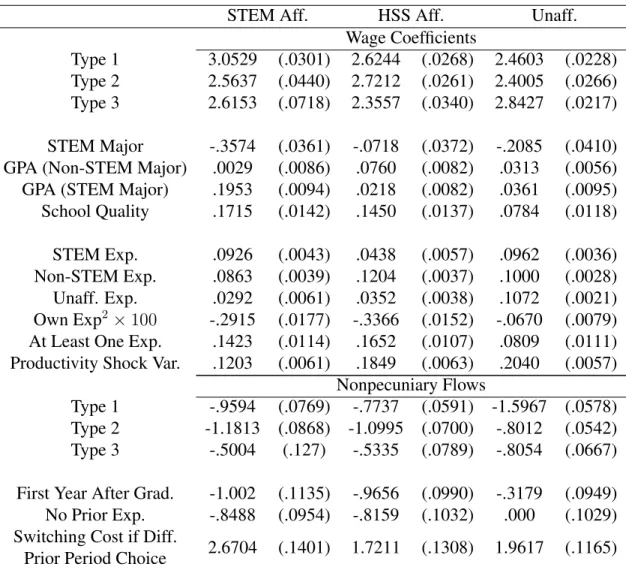
1.6.1 Labor Market

My estimates of the labor market coefficients are given in Table 1.4 for the skilled labor market

and Table 1.5 for the unskilled labor market. First note that the unobserved types of individuals

(θ1, θ2, θ3) each have a comparative productivity advantage for a particular labor sector (STEM,

HSS, unaffiliated, respectively). There is a strong degree of comparative advantage, especially for

type 1 in the STEM affiliated sector over other types, on the order of 0.45 log-wage units. There are

smaller but qualitatively similar productivity advantages for the other two types in their respective

23_{Given the high degree of persistence in occupation, empirical identification of returns to off-sector experience is}

Table 1.4: Skilled Labor Market Parameter Estimates by Occupational Sector

STEM Aff. HSS Aff. Unaff.

Wage Coefficients

Type 1 3.0529 (.0301) 2.6244 (.0268) 2.4603 (.0228)

Type 2 2.5637 (.0440) 2.7212 (.0261) 2.4005 (.0266)

Type 3 2.6153 (.0718) 2.3557 (.0340) 2.8427 (.0217)

STEM Major -.3574 (.0361) -.0718 (.0372) -.2085 (.0410)

GPA (Non-STEM Major) .0029 (.0086) .0760 (.0082) .0313 (.0056)

GPA (STEM Major) .1953 (.0094) .0218 (.0082) .0361 (.0095)

School Quality .1715 (.0142) .1450 (.0137) .0784 (.0118)

STEM Exp. .0926 (.0043) .0438 (.0057) .0962 (.0036)

Non-STEM Exp. .0863 (.0039) .1204 (.0037) .1000 (.0028)

Unaff. Exp. .0292 (.0061) .0352 (.0038) .1072 (.0021)

Own Exp2×100 -.2915 (.0177) -.3366 (.0152) -.0670 (.0079)

At Least One Exp. .1423 (.0114) .1652 (.0107) .0809 (.0111)

Productivity Shock Var. .1203 (.0061) .1849 (.0063) .2040 (.0057) Nonpecuniary Flows

Type 1 -.9594 (.0769) -.7737 (.0591) -1.5967 (.0578)

Type 2 -1.1813 (.0868) -1.0995 (.0700) -.8012 (.0542)

Type 3 -.5004 (.127) -.5335 (.0789) -.8054 (.0667)

First Year After Grad. -1.002 (.1135) -.9656 (.0990) -.3179 (.0949)

No Prior Exp. -.8488 (.0954) -.8159 (.1032) .000 (.1029)

Switching Cost if Diff.

2.6704 (.1401) 1.7211 (.1308) 1.9617 (.1165) Prior Period Choice

Note: Wage coefficients are reported in log-units of yearly thousands of dollars. Bootstrap standard errors are in parentheses.

sectors.

For each occupational sector, the returns to GPA are significantly higher if the major matches

the occupation: a 1.0 increase in GPA for STEM majors working in the STEM sector results in an

increase in wages by 0.195 log-units, while only 0.003 log-units for non-STEM majors working

in the STEM sector. A similar effect occurs for non-STEM majors in HSS occupations, while

in the unaffiliated sector the returns to GPA are similar and small for both majors. Considering

that the average terminal GPA of graduates in my sample is 3.38 for STEM and 3.15 for