M
ARKET-
TIMING ANDA
GENCYC
OSTS:
E
VIDENCE FROMP
RIVATEE
QUITYOleg Gredil
A dissertation submitted to the faculty of the University of North Carolina at Chapel Hill in partial fulfillment of the requirements for the degree of Doctor of Philosophy in the Department of Finance.
Chapel Hill 2015
Approved by:
Gregory W. Brown
Nickolay Gantchev
Eric Ghysels
Chotibhak (Pab) Jotikasthira
c 2015 Oleg Gredil
ALL RIGHTS RESERVED
ABSTRACT
OLEG GREDIL: Market-timing and Agency Costs: Evidence from Private Equity.
(Under the direction of Gregory W. Brown)
Private equity (PE) funds operate at the interface of private and public capital markets. This
paper investigates whether PE fund managers have private information about the valuations of
publicly traded securities. Using a dataset of cash flows from 941 buyout and venture funds,
I show that PE funds’ distribution patterns predict returns of public securities in the industries
of the funds’ specialization, but fund managers tend to sell at the market peaks only when they
have performance fees to harvest. I find that the cost of this agency tension increases in the
manager’s survival risk and that the managers’ knowledge pertains to the public firms’ future
earnings rather than the discount-rates. My tests distinguish market-timing from reactions to
the variation in risk premia and spillover effects of PE activity on public firms. The results help
better understand PE performance and have strong implications for PE manager selection. It
To my loving wife and children: Ekaterina, Vasilisa and Mark. Thank you for your continuing inspiration and support!
ACKNOWLEDGMENTS
I would like to especially thank Gregory Brown for his support and guidance. I am grateful
to my Dissertation Committee Members: Gregory Brown, Pab Jotikasthira, Nickolay Gantchev,
Eric Ghysels, and Christian Lundblad. Helpful comments and suggestions were provided by
Nicholas Crain, Victoria Ivashina, Steven Kaplan, Stas Khrapov, Cami Kuhnen, Paige Ouimet,
Urs Peyer, Adam Reed, Merih Sevilir, Morten Sørensen, Geoffrey Tate, William Waller and
seminar participants at the 2013 Global Private Investing Conference. I am grateful to Burgiss
for data access and to Wendy Hu for providing research assistance. This research has benefited
from the support of the Private Equity Research Consortium (PERC) and the UAI Foundation.
TABLE OF CONTENTS
1 INTRODUCTION . . . 1
2 DATA . . . 7
3 A SIMPLE MEASURE OF GPS’ MARKET TIMING . . . 12
4 HYPOTHESES AND METHODS . . . 19
4.1 Related Literature . . . 19
4.1.1 Pseudo-timing. . . 20
4.1.2 Footprints of PE Activity . . . 21
4.2 Hypotheses . . . 22
4.2.1 Are non-IPO Exits Informative? . . . 22
4.2.2 Exploring Agency Costs for Identification . . . 22
4.2.3 When Do Exits Convey Less Information? . . . 23
4.2.4 Potential Power Drains . . . 24
4.2.5 Combining Thoughts . . . 25
4.3 Research Design. . . 27
4.3.1 Identification Strategy . . . 28
4.3.2 Alternative Control Group . . . 30
5 MAIN RESULTS AND ANALYSIS . . . 33
5.1 Informed Exits Versus Uninformed . . . 33
5.1.1 Does Rush Hurt Holding Period Returns? . . . 39
5.2 Informed Rush versus Random . . . 43
5.2.1 Auxiliary Model . . . 46
5.2.2 Refining Base Estimates . . . 48
5.2.3 Evidence of Informed Stays . . . 50
5.3 What Are GPs Informed about: Cash-flows or Discount-rates? . . . 56
6 CONCLUSION . . . 60
A.1 Additional Data and Discussion of the Institutional Background. . . 62
A.2 Simulation-related Supplements and Discussions . . . 72
A.2.1 Recap and Robustness . . . 72
A.2.2 Alternative Approaches . . . 77
LIST OF TABLES
2.1 Summary Statistics . . . 9
3.1 Timing Track Record: Associations and Persistence . . . 17
5.1 Informed Rushversus Uninformed . . . 37
5.1 DoesInformed RushSacrifice Holding Period Returns? . . . 41
5.2 ActualRushversus Random . . . 49
5.3 Risk-shifting Evidence . . . 54
5.4 What Are PE Managers Informed About: Cash Flows or Discount Factor . . . 58
A.1 TTR Cross-Section: Robustness and Placebo . . . 69
A.2 Do Exits Cause Downturns? . . . 70
A.3 The Model of Fund Fixed Effects . . . 71
LIST OF FIGURES
2.1 Private Equity Fund Cash-flows: Cross-Section . . . 11
3.1 Timing Track Records: Sample Funds . . . 16
5.1 Informed RushandIndustry returns: Event Studies . . . 34
A.1 Private Information Cycle . . . 64
A.2 Timing Track Records: Examples . . . 65
A.3 Industry Returns and Fund Inceptions . . . 66
A.4 Timer’s Rush and Industry Returns: Additional Event Studies . . . 67
A.5 Timer’s Rush and Industry Returns: Quarterly Portfolios . . . 68
A.6 Actual Exits versus Simulated . . . 78
A.7 Robustness . . . 79
1 INTRODUCTION
Although by their nature private equity (PE) funds invest in private companies, their
per-formance often depends crucially on the interface with public capital markets. Whether or not
the fund’s exit (or entry) involves a public transaction, comparable public market valuations
affect the price. Prior research shows that PE managers are causing changes in policies of
the investee companies as well as the industries in which these companies operate in, while
being highly responsive to conditions in capital markets.1 Yet, there is little evidence of how
informed PE managers are about the valuations of public equities and what role this
informa-tion plays in their investment outcomes. In this paper, I examine whether PE managers can
really buy low and sell high. I rely on the agency of PE intermediation to identify a private
information-based market-timing from the alternative explanations. Since the counterfactual
with market-timing actions is relatively observable, I am also able to quantify some agency
costs of delegated money management. My results suggest that expected flows from future
funds restrain managers from “destroying value” (consistent with the theoretical framework of
Chung et al., 2011), but they fall short of inducing enough incentives.
Participation in private equity funds requires the investors (the limited partners, or LPs) to
provide a pre-specified amount of cash over a multi-year period on short notice. The schedule
of these outlays isex-anteunknown and determined by the managers of the funds (the general
partners, or GPs). In addition to fixed fees, GPs receive performance fees (carried-interest),
a fraction of the fund life-time profits, and decide when to return capital to LPs.2 Such a
near-absence of control over the timing of investments and divestments on the part of investors
distinguishes the private equity funds from other forms of delegated asset management. The
ceding of contribution and distribution timing to PE managers is commonly viewed as
nec-essary given that PE funds hold non-traded assets. Yet, the delegation of these rights is also
perceived as a source of liquidity risk for LPs. Recent studies have shown that GPs may be
extracting agency benefits from these control rights over the fund cash-flow schedule.3
Less understood is the potential benefit to LPs of ceding these cash-flow timing rights.4 GPs
specialize in certain types of businesses, know as much as the companies’ management and,
at the same time, have a first-hand read on the portfolio demands of financial and corporate
investors.5 Consequently, in this analysis I empirically focus on two closely-related issues.
First, I examine if PE managers have an informational advantage relative to public market
prices. I show that PE managers do appear to learn valuable private information about the
valuation of certain public equities and that the potential gains to LPs of delegating
cash-flow timing decisions to GPs can outweigh illiquidity costs. The economic magnitude of the
effect is large. An inter-quartile increase in the rate of funds’ distributions to investors predicts
approximately 6% lower 12-month returns for the fund’s primary S&P500 sector.
Second, I examine the effects of the agency relationship between LPs and GPs. I show that
unless GPs have “skin-in-the-game” via positive performance fees to harvest, they appear to
not be using their private information to exit the fund investments near the market peaks while
2Despite a large degree of flexibility, distributions are subject to contractual limits on the fund life which are typically 10 to 13 years since inception. While the period of possible capital outlays from investors is largely limited to the first 5 years since fund inception.
3See Robinson and Sensoy (2013), Phalippou (2009), Degeorge, Martin, and Phalippou (2013).
4PE fund managers oversee operations of dozens of companies. In comparison to most investors in public companies, PE managers are relatively unrestricted in information sharing with the companies’ managers.
not delivering better holding-period abnormal returns either.6 I also show that GPs with a good
market-timing track record, but nonetheless facing a particularly high survival risk (beyond the
current fund term), are more likely to delay distributions to LPs when industry return volatility
is about to rise.7 In these situations, GPs may decrease distributions because they own
out-of-the-money options on the current and future funds’ assets, and increasing industry volatility
makes these options more valuable. These results contribute to the growing literature on private
equity governance and, more broadly, on optimal contracting.8
I conduct my analysis using a sample of 941 U.S.-focused buyout and venture funds
in-cepted between 1979 and 2006. The data comes from the Burgiss database of private equity
funds that previous studies have found to be representative of the universe that has been
avail-able for institutional investors.9 Besides the precise amounts and dates of capital calls and
distributions for each fund, I observe quarterly net asset values as well as various
characteris-tics including GP-affiliation and the industry of specialization. My research design examines
public market return (mean and variance) predictability as a function of the relative size and
timing of PE fund distributions while accounting for the time-varying supply of mature funds
(i.e., those with portfolio companies that are ready for exits). Using difference-in-difference
tests, I disentangle the industry timing skills of GPs from alternative explanations such as
time-varying exit conditions or causal effects of PE activity on the public companies.
The key identifying assumption is that alternative explanations to the timing skill (or the
6Normally, performance fees in PE are subject to a claw-back if the fund’s remaining assets value decreases. Meanwhile, early exits may reduce the amount of asset management and monitoring fees that GPs collect from the fund, and also forgo a chance to improve the performance rank amongst peer-funds.
7These results obtain through the simulation-based estimation which controls for vintage-X-industry variation as well as other GP-specific and fund-specific attributes.
8For example, Barrot (2012) finds that remaining fund life determines the type of venture fund investments which can run counter to LPs’ objectives. Degeorge, Martin and Phalippou (2013) find evidence consistent with GPs “going-for-broke” with secondary buyout investments. On the other hand, the results in Fang, Ivashina, and Lerner (2014) suggest that GPs intermediation might not be as costly. The authors find essentially no outper-formance of private investments implemented by LPs directly while the co-investments run by GPs significantly underperform.
9See Harris, Jenkinson, and Kaplan (2013).
existence relevant private information) do not depend on the changes in a GP’s own wealth
exposure to the industry valuations. I verify this assumption via a series of placebo tests and
event studies. Consistent with the private information hypothesis, returns predictability from
fund cash flows vanishes outside of the industries in which the GPs specialize and relates
to the industry aggregate earnings news. I develop a new metric of GP’s cash-flow Timing
Track Record that contains valuable information about a fund’s future propensity to sell close
to industry highs and buy around lows. Consistent with the predictability being related to
GP skill, these market-timing track records appear to be just as important a signal as financial
incentives. To examine the robustness of my results and remove potentially confounding effects
in my primary tests, I conduct simulations that allow for a better control for variation in exit
conditions (e.g., time-varying expected returns by industry). The inference is robust to errors
clustered in calendar-time, as well as to exclusions of particularly dramatic market episodes
and certain fund groups.
While this paper is the first to directly examine the relation between PE manager private
information and public market returns, there exists anecdotal and indirect evidence consistent
with market-timing ability of PE managers (or, at least, efforts thereof).10 In a survey of 79
buyout firms by Gompers, Kaplan and Mukharlyamov (2014), “facilitating a high value exit”
is among the top three ways buyout funds seek to create value. Recently, prominent private
eq-uity firms have launched actively managed mutual funds citing their private investing expertise
as a managerial advantage.11 Yet, to-date there is no direct evidence supporting the PE
pri-vate information-based market-timing hypothesis, clear of the alternative explanations which
notably confound the economic implications of the results.12
10Anecdotal evidence of positive informational spillovers from investing in private companies includes exam-ples of successful public “stock pickers” that heavily invest in private companies: Warren Buffet of Berkshire Hathaway, Charles Coleman of Tiger Global, among many others.
11For example, see “Following KKR, Blackstone Chases Retail With Mutual Fund”, Forbes, 07/16/2013.
My findings suggest that an LP’s choice of a fund manager should incorporate a GP’s
market-timing track record since the expected gains persist across funds by the same GP and
are of the same order of magnitude as private equity illiquidity costs.13 However, to the extent
a given GP is at risk of not raising a next fund (e.g., due to lack of a long-term reputation),
the expected gains from market-timing decreases and may turn negative as the probability of
the aforementioned “asset-hoarding” increases. Provided that some GPs’ market-timing skill
would therefore require lower (or higher) liquidity premium for the funds they manage, my
analysis speaks to a few important questions in the investments literature: (i) why investors
choose to allocate to PE, (ii) how they select GPs, and (iii) what contract they have with a
particular GP.
As per Harris, Jenkinson and Kaplan (2013), the data indicate that in large samples, both
buyout and venture funds on average outperform public markets (on the holding period basis).
My findings suggest that the portfolio abnormal performance attributable to PE is likely even
better in aggregate, given the additional value from market-timing.14 However, the returns on
a strategy of picking the best PE managers from the past might be diminishing as suggested
by Harris, Jenkinson, Kaplan and Stucke (2013) as well as by Sensoy, Wang, and Weisbach
(2013). Both studies find less persistence in holding period returns by GPs and LPs than in
earlier samples.15 Thus, I contribute to the understanding of why LPs may still prefer PE fund
managers with the best past track records even if holding periods returns of their funds are not
much different from those run by less established competitors.16
13Franzoni, Nowak, and Phalippou (2012) and Sørensen, Wang, and Yang (2014) using very different ap-proaches estimate the illiquidity costs for PE to be 2-3% per annum. However, neither of the studies consider the cash-flow timing dimension of fund returns. Similarly in Ang, Chen, Goetzmann and Phalippou (2013), pri-vate equity time-varying abnormal returns capture only the portfolio company selection and nurturing effects (i., holding period returns).
14Even without active management on the part of an LP, private equity fund distributions near industry peaks induces fluctuations in portfolio weights that result in higher Sharpe-ratios for the LP. Meanwhile, LPs may also consider optimizing allocations in their public equity portfolio based on the signals from the private equity part.
15See Kaplan and Schoar (2005), and Lerner, Schoar, and Wang (2007).
16For example, LPs may do so because (1) they learn more market-timing signals from such GPs; (2) this
The results in this paper also imply broader roles for private equity in the modern
capi-tal markets. In settings such as Grossman and Stiglitz (1980), GPs’ learning through private
investing constitutes a “costly arbitrage” that improves the informational efficiency of public
markets. For example, the tech-bubble of the late 1990s might have gotten greater if not for
the flood of private equity exits trying to preempt (the GPs’ carried interest being hit by) the
bust. Specifically, venture funds incepted between 1995 and 1998 have divested considerably
more than invested during the later stage of the NASDAQ boom. Even for the funds with not
fully drawn capital commitments as of the beginning of 1999, the ratio of total distributions to
capital calls during the following 12 months was 7-to-1.17 This fact is hard to reconcile with a
popular wisdom that venture capitalists’ activity tends to amplify the valuation cycle.18
The dissertation proceeds as follows. Section 2 describes the data. Section 3 provides
pre-liminary evidence of the market-timing skill presence among private equity GPs and motivates
the hypotheses development and methods choice in Section 4 which also reviews the related
literature. Section 5 reports main results. Section 6 concludes. Additional details, robustness
and placebo tests are in the Appendix.
reduces the ex-ante probability of their GPs having difficulty with raising a follow-on fund and, thus, the afore-mentioned risk-shifting incentives.
17While the same ratio for the funds specializing inInternet Technologywas in excess of 9-to-1.
2 DATA
Private equity data for this study come from Burgiss, a leading provider of portfolio
man-agement software, services, and analytics to private capital investors. The dataset is sourced
exclusively from about 300 investors in private capital funds (LPs) that collectively have made
over 20,000 fund commitments, and includes the complete cash flow and valuation history with
these funds1 The underlying LP universe consists of approximately 60% pension funds (a mix
of public and private), 20% endowments and 20% other investors (such as sovereign wealth
funds and funds-of funds).2 Harris, Jenkinson, and Kaplan (2013) compare several private
eq-uity datasets and conclude that the Burgiss dataset is representative of the buyout and venture
funds investable universe.
I limit the sample to U.S.-focused buyout and venture funds with more than25and10
mil-lion in capital commitments (respectively) incepted between 1979-2006. In total, the sample
includes 349 (592) buyout (venture) funds of which 126 (169) continue operations as of March
2013. For each fund I observe: (1) the primary industry sector according to Global
Indus-try Classification Standard (henceforthindustry); (2) the amount of capital committed; (3) the
strategy description; (4) the dated amounts of cash inflows and outflows as well as Net Asset
Values (NAVs) reported quarterly.3
Panel A of Table 2.1 reports basic summary statistics for buyout and venture subsamples.
1Thus, the sample does not include co-investments or direct private investments studied in Fung et al.(2014).
2The dataset maintains confidentiality by removing all names and identifications.
The results suggest high within-type variation in fund life duration, size, and returns.4 85%
of funds are affiliated with a private equity firm (GPs) with multiple funds. For these funds, I
observe the fund’s chronological order (by inception date) within GP and GP-industry.5 Thus,
the median fund in the dataset is the second by a GP and within a given industry while about
a quarter of funds are fourth or higher in a sequence. Mature venture GPs are somewhat less
likely to operate in multiple industries, unlike those specializing in buyouts.
4Returns are as of the last cash flow or valuation date in the sample.
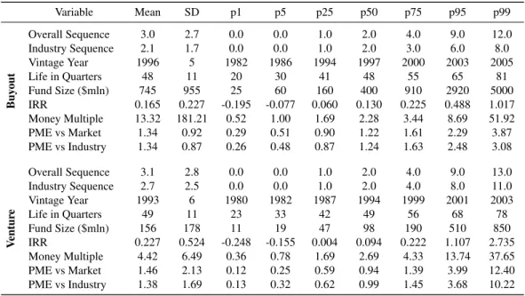
Table 2.1:
Summary Statistics
This table reports summary statistics for the data used in this study. Panel A reports sequence order, vintage year, life since inception, size, and the last-most performance statistics for 349 (592) U.S.-focused buyout (venture) funds of which 126 (169) continue operations as of March 2013. OverallandIndustry Sequencereport the fund chronological order of the inception date within GP and GP-industry respectively or zeros when fund’s GP data is not available ( 15% of sample funds). IRR stands for internal rate of return. PME vs Market (Industry) denotes Kaplan and Schoar (2005) Public Market Equivalent Index versus broad market (S&P500 subindex corresponding to the GICS Industry Sector of the fund specialty). Panel B reports statistics for monthly returns, price-to-earning-and book-to-market-ratios of these subindexes for the period from January 1989 through October 2013. Panel C reports statistics for the rest of the variables as described in Section 4.2.
Panel A:Private Equity Funds
Variable Mean SD p1 p5 p25 p50 p75 p95 p99
Buy
out
Overall Sequence 3.0 2.7 0.0 0.0 1.0 2.0 4.0 9.0 12.0
Industry Sequence 2.1 1.7 0.0 0.0 1.0 2.0 3.0 6.0 8.0
Vintage Year 1996 5 1982 1986 1994 1997 2000 2003 2005
Life in Quarters 48 11 20 30 41 48 55 65 81
Fund Size ($mln) 745 955 25 60 160 400 910 2920 5000
IRR 0.165 0.227 -0.195 -0.077 0.060 0.130 0.225 0.488 1.017
Money Multiple 13.32 181.21 0.52 1.00 1.69 2.28 3.44 8.69 51.92
PME vs Market 1.34 0.92 0.29 0.51 0.90 1.22 1.61 2.29 3.87
PME vs Industry 1.34 0.87 0.26 0.48 0.87 1.24 1.63 2.48 3.08
V
entur
e
Overall Sequence 3.1 2.8 0.0 0.0 1.0 2.0 4.0 9.0 13.0
Industry Sequence 2.7 2.5 0.0 0.0 1.0 2.0 4.0 8.0 11.0
Vintage Year 1993 6 1980 1982 1987 1994 1999 2001 2003
Life in Quarters 49 11 23 33 42 49 56 68 78
Fund Size ($mln) 156 178 11 19 47 98 190 510 850
IRR 0.227 0.524 -0.248 -0.155 0.004 0.094 0.222 1.107 2.735
Money Multiple 4.42 6.49 0.36 0.78 1.69 2.69 4.33 13.74 37.65
PME vs Market 1.46 2.13 0.12 0.25 0.59 0.94 1.39 3.99 12.40
PME vs Industry 1.38 1.69 0.13 0.32 0.62 0.99 1.45 3.68 10.22
Panel B:Industry Benchmarks
GICS Sector Returns Book-to-Market Price-to-Earnings
Mean SD Skew Mean p25 p75 Mean p25 p75
Consumer Discre-tionary
0.009 0.052 -0.737 0.379 0.319 0.438 27.0 15.7 22.9 Consumer Staples 0.009 0.040 -1.047 0.238 0.178 0.291 20.1 15.9 21.1 Energy 0.010 0.053 -0.397 0.438 0.358 0.521 17.6 12.4 19.4 Financials 0.007 0.065 -0.984 0.629 0.467 0.840 24.6 12.8 17.7 Healthcare 0.010 0.047 -0.461 0.247 0.165 0.320 20.0 15.9 21.3 Industrials 0.009 0.046 -1.107 0.323 0.283 0.369 23.3 16.7 27.2 Internet Technology 0.008 0.072 -0.796 0.327 0.224 0.451 27.5 15.2 35.6 Materials 0.008 0.057 -0.627 0.424 0.359 0.460 23.6 14.8 28.4 Telecommunications 0.007 0.055 -0.402 0.406 0.280 0.509 21.0 15.6 23.0 Utilities 0.008 0.044 -0.616 0.554 0.484 0.678 15.2 12.3 16.7
Panel C:Other Variables
Variable Mean SD p1 p5 p25 p50 p75 p95 p99
Market Return (*100) 0.92 4.58 -10.22 -7.60 -1.74 1.52 3.93 7.66 10.20 CAY Ratio (*100) 0.26 2.28 -3.35 -3.13 -2.04 0.52 2.25 3.46 3.96 CBOE VIX 20.7 7.8 11.1 11.8 15.3 19.4 24.1 35.1 46.4 BBB-AAA spread 0.99 0.40 0.55 0.60 0.75 0.91 1.16 1.46 3.00 AAA-UST spread 1.32 0.48 0.49 0.71 0.90 1.24 1.69 2.12 2.53 10-year yield (*100) 5.55 2.01 1.68 1.98 4.10 5.50 7.17 8.86 9.26 3-month yield (*100) 3.69 2.41 0.02 0.05 1.33 4.34 5.40 7.69 8.43
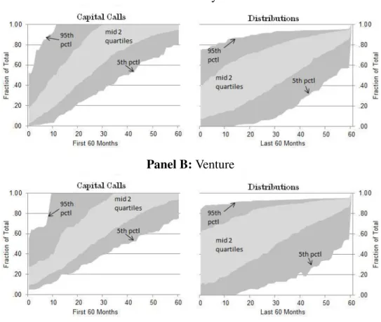
Figure 2.1 demonstrates high variation in fund cash-flow schedules for both buyout and
venture funds. As shown in Panel A, a quarter of buyout funds call 61% or less of committed
capital by the 30th month since inception while another quarter are fully invested by that time.
Distributions from buyout funds are even more variable. Among buyout funds, a quarter had
40% of total distributions completed 30 months prior to resolution whereas another quarter
had over 80% distributed.6 Panel B reports similar charts for venture funds and indicates even
wider variation in both contributions and distributions.
I utilize the CRSP value-weighted index as a proxy for public market equity returns. For
equity industry returns, I use returns on S&P500 industry sectors because these map directly
to the classification in the Burgiss data and represent widely-followed benchmarks by
practi-tioners.7 The list of industries and summary statistics for monthly total returns, price-earnings
and book-to-market ratios from January 1989 through September 2013 are reported in Panel B
of Table 2.1. Panel A of Table 2.1 also reports the PME measure of market-adjusted fund
per-formance as described by Kaplan and Schoar (2005), as well as a similar indicator calculated
against the industry benchmarkPME vs. Industry.8 Summary statistics for other variables of
6I define “resolution” as funds older than 5 years since inception with remainingN AV ≤1%of fund size. 7Results are similar if I use industry subindexes of the S&P600 (small capitalization stocks).
Figure 2.1:
Private Equity Fund Cash-flows: Cross-Section
This figure reports the 5th, 25th, 75th, and 95thpercentiles for the fraction of to-date capital calls (distributions) in the total amount eventually to be called (distributed) by each fund during the first (last) 60 months of its operation. Panel A plots results for the buyout subsample. For example, according to the left-chart, a quarter of buyout funds by the 30th month since inception would call 61% of its capital or less while another quarter would be fully invested by that time. From the right-chart we learn that among almost fully resolved buyout funds, a quarter had about 40% of total distributions completed 30 months before last while another quarter had over 80% already distributed. Panel B reports this analysis for the venture subsample.
Panel A:Buyout
Panel B:Venture
interest are reported in Table 2.1 Panel C.CAY Ratiois the cointegrated consumption-wealth
ratio from Lettau and Ludvigson (2001). VIX is the CBOE volatility index for the S&P500.
BBB-AAA spreadandAAA-UST spreadare, respectively, difference between Moody’s Baa and
Aaa yields, and Aaa yield and 10-year constant maturity U.S. Treasury yield, 10-year yield.
3-month yieldis the U.S. Treasury bill rate.
3 A SIMPLE MEASURE OF GPS’ MARKET TIMING
The information that a GP obtains through the investment cycle and public markets
valu-ations are closely related.1 Public markets prices reflect cash flow expectations and investor
preferences while also affecting the fund’s investment entry and exit prices, regardless of the
deal sourcing and exit route. As an example, consider an exit through a sale to a public
corpora-tion. Bargaining over price would normally evolve around an assortment of valuation ratios of
comparable publicly traded firms as indications of a fair price, even though the business
char-acteristics might not exactly match those of the target company. Thus, GPs may be able to take
advantage of superior knowledge of industry trends even when the fund portfolio companies
have, in fact, relatively small exposures to these trends.
The ability of GPs to act on company-specific information advantage is likely to be
lim-ited by adverse-selection concerns of the prospective buyers. A need to make concessions
with regards to idiosyncratic returns would be consistent with buyout- and venture-backed
IPO outperformance, particularly against characteristics-matched portfolios, as documented in
Brav and Gompers (1997), Cao and Lerner (2006), and Harford and Kolasinski (2013).
How-ever, this adverse selection is much less relevant with regards to industry-wide risk realizations
since those who typically buy from (sell to) private equity funds care more about the relative
performance of the asset, not absolute performance as do private equity GPs.2 In general, GPs
informational advantage should dissipate beyond the industry of specialization.
I begin my analysis with suggestive evidence that GP access to information relevant to
1A detailed discussion of the institutional details supporting this statement is provided in Appendix A.1.
industry valuations manifests in PE fund cash flows. To analyze the timing track records and
obtain a proxy for a presence of such a skill, I propose a measure of a gross return over a
fund’s life-time due to selling at market highs and buying at market lows. Computationally it
is very similar to the Public Market Equivalent (PME) of Kaplan and Schoar (2005). However,
the Timing Track Record (henceforth TTR) measures the timing component of a fund’s total
returns thatPMEexplicitly disregards. Specifically, I define,
T T R
=
P M E
P M E
=
PT
t=1Dte
r1,T·(1−t/T)
/
PT1 Cte
r1,T·(1−t/T)
PT
t=1Dtert,T
/
PT1 Ctert,T
(3.1)
where rt,T is the market return from the cash flow date (t) until the fund’s resolution (T),
while Dt(Ct) denotes the fund’s distributions (capital calls). In essence, TTR is a ratio of
two profitability indexes with different discount rates. The discount rates in the denominator
reflectinvestment periodsopportunity costs while the discount rates in the numerator reflects
thecommitment periodopportunity costs. Thus, aTTRvalue above one indicates that the NPV
is greater if measured against the fund commitment period opportunity cost. In other words, a
TTR greater than one is consistent with value-added from the market-timing by GP.3 Just as
PME,TTRcan be computed on a to-date basis by assuming the respective period to be the last
and the NAV at that date to be a liquidating distribution. See Brown, Gredil, and Kaplan (2013)
for to-date-PME definitions. Importantly, the mean market return forP M E computation will
also be last date specific.
To better understand the intuition behind TTR, consider the following stylized example.
Two funds, A and B, start at the same time with $30 in committed capital and have to 2 years
to invest. Both funds liquidate at year 4. For simplicity we assume that neither fund has
portfolio company selection skill and so earns the market rate of return on investments, thus
3Also,ln(T T R)/F undDurationcan be viewed as the annual rate of timing alpha.
PME=1.0 for both funds by definition. However, fund A chooses to draw capital in equal
installments over 3 years whereas fund B, correctly anticipating a market downturn, draws less
capital initially.
Entry Timing Example
Year rmkt Fund ACash Flow Fund BCash Flow Fund ANAVs
0 - -10 -5 10
1 5.0% -10 -5 20.50=10·1.05+10
2 -13.6% -10 -20 27.71
3 5.0% 0 0 29.09
4 5.0% 30.55 31.81 0
P M E 1.00 1.00
P M E 1.02 =30.55/30 1.06 =31.81/30 T T R
T T R
T T R=P M E/P M E 1.02=1.02/1.00 1.06=1.06/1.00
While both funds havePMEequal to one, fund B creates more value for its LPs than fund
A: 1.81 versus 0.55. This added value is reflected in a higher P M E for fund B and thus a
higherTTR for fund B. In this way TTRmeasures the market timing ability of the managers
of fund B. Appendix A.2 provides examples with more realistic cash flows and market returns
that show howTTRcaptures the timing of exits as well.
The money-multiple (i.e., ratio of nominal distributions to contributions) is an absolute
per-formance measure widely utilized by practitioners and would reflect the difference in returns
to LPs from funds A and B. In fact, the money-multiples of A and B are 1.02 and 1.06,
respec-tively. In this specific case, they are the same asTTRs because the cumulative market return
is zero and the PME of each fund is 1.0. However, in practice money-multiples also reflect
differences in market returns over fund lives, as well as differences in fund holding period
ab-normal returns. Thus, Equation (3.1) essentially strips-out the prevailing market trend from the
money-multiple and deflates it by the gross life-time return due to portfolio companies’
to risk misspecification by virtue of its relation toPME. 4 Specifically, risk-related errors will
tend to cancel out in TTR because P M E will have beta-related estimation errors positively
correlated with those in PME.
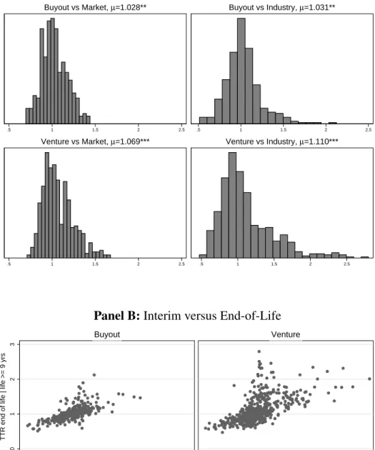
Panel A of Figure 3.1 plots distributions of end-of-lifeTTRs for the sample funds against
the broad market and the respective fund industry, separately for buyout and venture
subsam-ples. First, the dispersion of TTR is comparable with that of PME, suggesting that TTR is
indeed a potentially important dimension of fund performance. Second, the means are
statis-tically different from one and are larger for the industry benchmark case albeit the distances
are economically small, corresponding to average industry timing alpha of about 1% per year
since inception.5 Nonetheless, almost a third of funds in both subsamples have aTTRof 1.18 or
higher which exceeds the 2% per year “break-even” alpha estimates in Sørensen et al.(2013).
Panel B of Figure 3.1 plots to-date TTRsas of the 5th anniversary against the end-of-life
TTRs(for funds that exist at least 9 years). By the 5th yearTTRwould tend to reflect mostly the
entry timing. Examples in Figure A.2 suggest that bad exit timing can offset the effect of the
entry and vice versa. Nonetheless, from Panel B it appears that funds that have a good timing
track record as of mid-life normally continue to do so through the remainder of their lives and,
thus, tend to exhibit good exit timing.
Panel A of Table 3.1 reports associations of industry TTRs with GP characteristics that
proxy for institutional quality.6 Fund size (size-squared) is positively (negatively) related to
end-of-lifeTTR. However, the size effect is insignificant when temporal variation is controlled
for through vintage year fixed effects. Fund sequence is positively related to TTRcomputed
using industry returns indicating that funds raised by GPs with more experience in a given
industry are likely to better navigate industry peaks and troughs. These results are not present
4See Korteweg and Nagel (2013) and Sørensen and Jagannathan (2013) for details. Robinson and Sensoy (2011) provide empirical assessment of the question by examining sensitivity of cross-sectional meanPMEto different beta/benchmark assumption).
5SinceTTRis limited by the benchmark volatility over the period, Sharpe-ratios may be more comparable across time and industries.
6See, for example, Kaplan and Schoar (2005), Robinson and Sensoy (2011).
Figure 3.1:
Timing Track Records: Sample Funds
This figure plotsTiming Track Record(TTR) values for the sample private equity funds.TTRis defined in Section 3 and measures the gross-return due to selling near the market peaks during the fund life-time and buying near the troughs. Panel A plots univariate distributions. Top-left (right) chart showsTTRsagainst the broad market index for the buyout (venture) funds, while bottom-left (right) charts showsTTRsfor the respective subsample against (S&P500 subindex of) GICS industry sector that the respective fund specializes in (Industry TTRs). Panel B compares end-of-5th-year and finalIndustry TTRsvalues for the buyout (venture) subsamples of funds that were for at least 9 years old.
Panel A:End-of-Life Values
.5 1 1.5 2 2.5
Buyout vs Market, m=1.028**
.5 1 1.5 2 2.5
Buyout vs Industry, m=1.031**
.5 1 1.5 2 2.5
Venture vs Market, m=1.069***
.5 1 1.5 2 2.5
Venture vs Industry, m=1.110***
Panel B:Interim versus End-of-Life
0
1
2
3
.5 1 1.5 2 .5 1 1.5 2
Buyout Venture
TTR end of life | life >= 9 yrs
for broad market returns reported in Panel B.
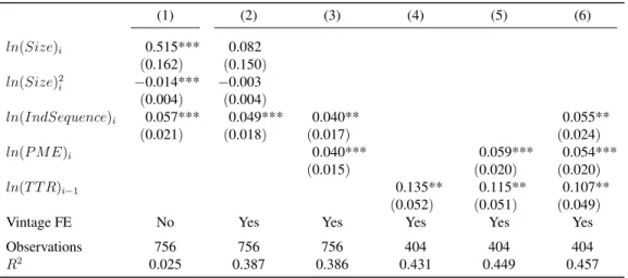
Table 3.1:
Timing Track Record: Associations and Persistence
This table reports linear regression model estimates of the log of funds’ end-lifeTTRs.TTRis defined in Section 3 and measures the gross-return due to selling near the market peaks during the fund life-time and buying near the troughs. The explanatory variables are: ln(Size)i (ln(Size)2i) - log (log-squared) of the fund $ capital
committed; ln(Sequence)i - chronological order of the fund inception date by given GPs (the private equity
management firm); ln(P M E)i- log of the fund’s Kaplan and Schoar (2005) Public Market Equivalent Index; ln(T T R)i−1- log of the GP’s previous fundTTR. In Panel ATTR,ln(Sequence)iandPMEare measured with
respect to the GICS Industry Sector of the fund specialty while in Panel B - versus the broad market/ all funds by given GPs. Specifications (2) through (6) include fund vintage-year fixed effects. Standard errors in parentheses are clustered by GPs, */**/*** denote significance at 10/5/1% confidence level.
Panel A:TTR versus Industry
(1) (2) (3) (4) (5) (6)
ln(Size)i 0.515*** 0.082
(0.162) (0.150)
ln(Size)2
i −0.014*** −0.003
(0.004) (0.004)
ln(IndSequence)i 0.057*** 0.049*** 0.040** 0.055**
(0.021) (0.018) (0.017) (0.024)
ln(P M E)i 0.040*** 0.059*** 0.054***
(0.015) (0.020) (0.020)
ln(T T R)i−1 0.135** 0.115** 0.107**
(0.052) (0.051) (0.049)
Vintage FE No Yes Yes Yes Yes Yes
Observations 756 756 756 404 404 404
R2 0.025 0.387 0.386 0.431 0.449 0.457
Panel B:TTR versus Broad Market
(1) (2) (3) (4) (5) (6)
ln(Size)i 0.164* 0.002
(0.085) (0.072)
ln(Size)2
i −0.005** −0.001
(0.002) (0.002)
ln(Sequence)i 0.048*** 0.034*** 0.015* 0.011
(0.009) (0.008) (0.009) (0.014)
ln(P M E)i 0.037*** 0.044*** 0.043***
(0.007) (0.010) (0.010)
ln(T T R)i−1 0.108** 0.093* 0.093*
(0.055) (0.049) (0.050)
Vintage FE No Yes Yes Yes Yes Yes
Observations 756 756 756 404 404 404
R2 0.035 0.468 0.482 0.470 0.516 0.517
One may suspect that market-timing is a substitute for GP skills required to select and
nurture fund portfolio companies. The positive coefficients forPME in specifications (3), (5)
and (6) suggest the opposite: funds with good “selection and nurturing” skills, as measured
byPME, tend to also be better at timing the industry cycles. Specifications (4) through (6) in
Table 3.1 show a positive relation between a GP’s previous fund’sTTRand the current fund’s
TTR. This is evidence that timing ability is persistent at the GP level. The fact that all of these
relations are uniformly weaker when timing is measured against the broad market benchmark
(Panel B of Table 3.1) is consistent with greater timing ability by GPs at the industry level. 7
In summary, this section has developed a simple but potentially powerful measure of GP
market timing ability. Timing ability appears to have significant positive value to LPs.
Further-more, it appears more related to industry returns than to market returns and is persistent at the
GP level. I now turn to a more detailed discussion of hypotheses, development of empirical
tests, and a discussion of results.
4 HYPOTHESES AND METHODS
4.1 Related Literature
The question of market timing by private owners connects to a large body of literature on
initial public offerings (IPOs) and mergers and acquisition (M&A) waves in the context of
either adverse selection (signalling) problems or some form of investor irrationality.1
How-ever, there are few studies of market timing track records of institutional money managers that
specialize in investing in private companies with an explicit horizon for exit.
Lerner (1994) examines the choices of venture-backed biotech firms to raise capital by
IPO or through private financing during 1978-92. He concludes that venture capitalists can
time the market by issuing before the sector declines and that experienced VCs appear more
skilled in this way. More recently, Ball, Chiu, and Smith (2011) argue that the biotech
sample-period of Lerner (1994) was anomalous. Using data on 3,477 IPOs and 4,486 acquisitions
of venture-backed companies over 1978-2009, they find evidence consistent with firms
react-ing to favorable exit conditions (“pseudo-timreact-ing”) rather than attemptreact-ing to take advantage of
investor over-optimism. This conclusion is based on the lack of evidence that IPOs precede
negative market/sector return as well as IPO returns being statistically lower than those after
exits through M&A. Kaplan and Str¨omberg (2008) summarize empirical evidence consistent
with buyout GPs taking advantage of market timing, including the relative (mis)pricing
be-tween debt and equity. Combining the results of Kaplan and Stein (1993), Axelson et al.(2010)
and Guo et al.(2011), the authors report expansion of the industry capital-to-cash-flow ratios
as an important driver of the mean absolute returns for the sample of buyout deals undertaken
in 1980-2006. Kaplan and Str¨omberg (2008) also elaborate on much higher responsiveness of
buyout leverage to the credit market conditions as opposed to that of public corporations which
may point to GPs’ ability to capitalize on apparent debt mispricing.2
4.1.1 Pseudo-timing
There are two alternative explanations to the market timing skill of GPs that are also
con-sistent with PE fundsTTR exceeding one and persisting (as per Section 3). First, GPs do not
have any superior information but a rush-to-exit reflects the variation in broad market and
in-dustry condition for exits, consistent with rational (yet uninformed) behavior models of Schultz
(2003) and Pastor and Veronesi (2005).3 Following Ball et al.(2011), I refer to this alternative
asPseudo-timing.4 Simply put, a “sell after market run-ups” trading rule can be implemented
without the costly help of the agent.
In fact, such investment timing by GPs may even generate utility losses to LPs since asset
valuations may reflect time-varying risk premia. One way to conceptualize this possibility is
with the notion of cash flow liquidity risks that LPs have to bear (e.g., with regards to yet
undrawn commitments that may not be offset by the distributions from other funds in the
portfolio). The cash squeeze that many endowments and pension funds endured in the 2008
financial crisis has sparked a research interest in liquidity premia appropriate for private equity
investing.5
It is important to realize that gains from Pseudo-timing do not provide a compensation
2Recently, Ang, Chen, Goetzmann and Phalippou (2013) reconfirm this capital market segmentation hypoth-esis having extracted the private equity time-varying excess return from pools of fund cash-flows via a Bayesian MCMC estimation.
3Schultz (2003) demonstrates that mean-reversion coupled with a decision rule of issuing after market run-ups would be observationally similar to informed trading. Pastor and Veronesi (2005) develop a model of “rational IPO waves” where issuance volume varies endogenously as a function of market conditions without any overreactions by investors or differences in cash-flow signal precisions.
4Although we adjust theTTRnumerator for the fund lifetime mean market return, it generally does not equal the expected market return in each period.
for these risks. To see this, consider an extension of the Merton portfolio choice framework
that encompasses liquid and illiquid risky assets as per Ang, Papanikolau, and Westerfield
(2011).6 The authors model illiquidity as the stochastic arrival of trading opportunities so
that immediate consumption can only be financed with liquid wealth (either risky or risk-free
asset). The likelihood of a suboptimally high weight of the illiquid risky asset in states of
high marginal utility of consumption causes lower target allocations to risky assets overall and
the illiquid one (i.e. private equity) specifically. Therefore, if private equity weights were to
increase in these high marginal utility states (i.e. as a result ofPseudo-timing), the equilibrium
expected returns required to support a given target allocation to the illiquid asset would need
to be higher.7 Hence, to assess the economic value-added from market-timing by GPs, it is
necessary to separate any such gains from thePseudo-timingalternative.
4.1.2 Footprints of PE Activity
The second group of alternative explanations pertain to the causal effect of private equity
fund operations on the behavior of public firms and investors. A number of recent studies
document evidence consistent with the peer firms responding to governance threats by changes
in investing and operating policies.8 In particular, Aldatmaz (2012) finds that private equity
investments cause financial and operating changes in publicly listed firms in the same
country-industry. Thus, it could be that the industry cash flow prospects change because private equity
funds alter their industry participation. I call thisFootprint-on-firms.
Both channels, market-timing and Footprint-on-Firms, may give rise to observationally
6The key implications are (i) higher allocation to risk free asset, (ii) low and path-dependent substitutability between liquid and illiquid assets, (iii) lower post-rebalancing weights of illiquid asset than a long-term optimal allocation.
7Similarly, private equity distributions in states of low marginal utility of consumption are more likely to be reinvested in the liquid risky asset which attenuates the positive effect of timely exits (as the avoidance of period of low market returns).
8See Berstein, Lerner, Sørensen and Str¨omberg (2011), Aldatmaz (2012) in context of private equity partic-ipation; Gantchev, Gredil, and Jotikasthira (2013) in context of hedge fund activism. Bernstein et al.(2011) and Aldatmaz (2012) consider the effect of private equity funds’ participation on the country-industry performance and find that increases in private equity participation lead to higher productivity and employment growth, contrary to a popular belief that private equity simply takes away from the surplus of other stakeholders.
similar event-time patterns. It could be also aPrice Distortion. That is, the market price may
temporarily decrease to absorb the increased supply of certain types of assets coming from
admittedly informed investors (i.e., private equity GPs), whereas the industry down-turn fails
to materialize. Note that neither Footprint-on-Firms nor Price Distortion necessarily imply
gains to LPs from GPs’ cashing-in earlier.
4.2 Hypotheses
In light of the discussion above, it is necessary to rely on cross-sectional tests to disentangle
the effect of market-timing and the associated gains to LPs from the alternative explanations.
The traditional route in the literature has been to compare IPO exits with other exits.9 However,
this cross-sectional approach may not be the best for examining GP market-timing ability.
4.2.1 Are non-IPO Exits Informative?
Consider a hypothetical 7-year old buyout fund that has yet to liquidate most of its
invest-ments. Suppose the GP anticipates the industry-wide cash flows will be notably below market
expectations in the near term but healthy in the long-run. Assume there is another fund
ap-proaching the end of its investment period that has yet to deploy its capital. GPs of the second
fund may agree to buy the holdings of the first fund at prices close to publicly-traded
compa-rables. They may in fact do so while fully sharing the belief about an upcoming downturn and
yet still be taking the first-best action from their LPs’ perspective.10 Hence, the exits by the
first fund would be informative of industry return expectations even absent an IPO. Likewise,
corporate buyers may have different investment horizons from that of the seller. Thus, exits
through trade-sale may be as informative about GPs’ expectations as sales through an IPO.
4.2.2 Exploring Agency Costs for Identification
The assumption that GPs take first-best actions for LPs is a strong one. Robinson and
Sensoy (2013) find that PE funds’ distributions cluster too much around “waterfall” dates for
9For example, Lerner (1994), Ball et al. (2011)
that assumption to be realistic. But, the conditional revelation of the GP’s private signal could
result precisely from the agency relationship. Continuing with the previous example of a 7-year
buyout fund, assume that the fund has performed well enough for GPs to have a substantial
performance fee in that fund. If fund investment value deteriorates at the end of the fund
contractual term (e.g. 10-12 years), the carried interest may vanish too. By rushing to sell the
fund holdings, not only do GPs secure performance fees, but they also lock-in a relatively high
performance rank among peer funds which can help attract investors in future funds.11
In contrast, there is hardly any benefit to GPs from exiting investments before the industry
downturn if the performance to-date is poor. Asset liquidation would amount to suboptimal
early-exercise of an option (to earn carry and improve performance rank) and reduce asset
management fees.12 Therefore, it is possible that skilled GPs facing such a survival risk would
likely seek to retain fund assets ahead of the turbulent times for the same reason that
option-holders want the underlying asset volatility to increase. However, since such an asset hoarding
may tarnish GPs’ reputation with investors and adversely affect future fundraising, one would
expect it to be limited to GPs that face immediate survival risk only (i.e. were unable to raise a
follow-on fund). That would be also consistent with the framework of Chung et al. (2011) as
well as empirical finding by Aragon and Nanda (2011) in hedge funds context.
4.2.3 When Do Exits Convey Less Information?
Suppose that our hypothetical fund has performed very well but already divested its best
deals (i.e. those yielding the highest performance fees). The remaining holdings in the fund’s
portfolio would then likely be comprised of the deals that failed to payout well. Provided that
the fraction of this residual in the total distributions to date is small, its option value (which
increases in the assets idiosyncratic risk as well) may still dominate any expected loss of value
to the fund’s carry amount due to the likely deterioration in the industry-wide factors.
11Chung, Sensoy, Stern, and Weisbach (2011) show that much of GPs’ wealth derives from fees in not yet raised funds.
12Some funds have the basis for asset management fees switching from committed to invested capital after the investment period elapses. See Robinson and Sensoy (2013).
Thus, as the value of the residual fund assets gets small in front of the amount of carry
already cashed-in, the incentive for GPs to reveal a negative market-timing signal diminishes.
Meanwhile, a low pace of distributions over the remainder of the fund’s life is also consistent
with a scenario when GPs have been expecting improvements in the comparable valuations
during that period (i.e., may contain a positive market-timing signal).13
Similarly, the divestments undertaken earlier in the fund’s life, while the residual exposure
of GP’s carried interest has remained high (or very little carry accrued yet), should contain
relatively less of the market-timing consideration. Such differences in the exits motives that
depend on the phase of the funds’ life naturally yield settings for placebo tests.
4.2.4 Potential Power Drains
Even if the incentives to act on the timing signal are in place, the signal may not arrive or
some GPs may not notice it (e.g., because of lower skill). Also, GPs might be too diversified or
could hedge their undesired exposures elsewhere.14 Prior research suggests that persistence in
GP performance is particularly strong in the worst quartile of funds.15 The substantial
hetero-geneity of PE fund returns is a statement about the high total risk of these funds, but also allows
for considerable heterogeneity in GP skill levels. Gervais and Strobl (2012) study the industrial
organization of asset management and show that in equilibrium high-skill and low-skill
man-agers pool into opaque funds, while medium-skill manman-agers separate into transparent funds. It
is hard to find a less transparent example of delegated money management than private equity.
13As industry-wide returns improve (yet remain small in front of the assets’ idiosyncratic returns), the exit choice will be increasingly driven by positive realizations of the idiosyncratic risks which, by definition, are uncorrelated across the assets. Hence, the remaining exits would be less clustered in time, all else equal. Equiva-lently, there will be fewer distributions per unit of time.
14However, finance professionals are often legally prohibited to undertake any personal investing activities potentially jeopardizing best actions in the interests of clients or their employer. There is little evidence suggesting how strong and common such clauses are but GP risk-aversion combined with basis risk could also limit these hedging activities.
4.2.5 Combining Thoughts
The evidence of successful cash-flow timing track records by PE funds presented in Section
3 combined with the discussion in this section yields the following hypotheses:
H1 : PE managers have valuable private information about public equity valuations (i.e., GPs
areInformed).
In other words, some GPs can predict returns of certain public equities because of a superior
information about either future cash-flows of these firms, or investors’ portfolio demands for
such assets, or both. However, in any sample there will be funds that ex-post timed market
peaks and troughs (better than others). Therefore, for a cross-sectional test of this hypothesis
one needs anex-anteindicator of fund market-timing skill (i.e., to defineInformedGPs versus
not). I will use fund TTR-to-date for this purpose and focus on the fund primary industry
valuations which allow for a sharper focus on the learning channel than market-wide returns.
IfH1holds, ceding the cash-flow timing rights to GPs may result in additional benefits to LPs
(or costs). Acorollary to H1is that TTRpersists across funds by the same GP as shown in
Table 5.1.
H2 : High rates of fund distributions predicts lower market returns when the value of GP’s
carried interest is at risk.
That is, the benefits of ceding the cash-flow timing rights to GPs are more pronounced
when such actions are more concordant with GPs wealth maximization. Acorollary toH2is that when a GP is either not Informed or not incentivized, the fund distributions do not
pre-dict market returns. I will proxy for GPs’ carried interest accrual (the “skin in-the-game”)
by levels of the fund net-of-fees performance to date, assuming 0 (8%) hurdle rate for
ven-ture (buyout) funds. If this hypothesis holds, we can conclude that (i) the agency aspect of
the GP-LP relations is important for PE fund performance (possibly even beyond the
market-timing dimension), (ii) nonetheless, LPs should expect the market-market-timing by GPs to positively
contribute to PE fund returns (to the extent that GPs are expected to earn positive carry).
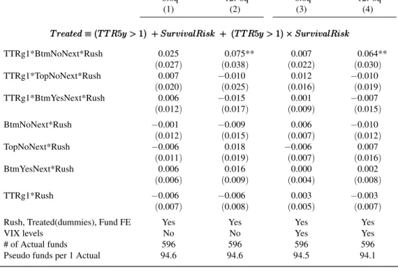
H3 : Risk-shifting behavior by anInformedGP is more likely to have an adverse effect on LP
portfolios as compared to risk-shifting behavior of anuninformedGP.
GPs may seek to retain fund assets ahead of elevated market volatility when their survival
is jeopardized. As discussed above, GPs are option-holders that want the underlying asset
volatility to increase. Provided that high volatility is typically associated with low returns, these
actions (when successful) would tend to result in lower Sharpe-ratios for LPs. The question is
whetherinformedGPs are more successful in correctly predicting such turbulent times in the
industry (while being as incentivized as their uninformed peers). If the answer is yes,informed
GPs will be a drag on LP portfolio performance.
There are two corollaries to hypothesisH3. H3A- when below the performance fee hurdle,
informedGPs create less value to their fund investors through holding period abnormal returns
thanuninformedGPs. H3B- informedGPs that have had poor current fund performance but
do not face immediate survival risk are less likely to engage in risk-shifting.
If H3 holds while H2 fails, PE funds in general may command higher risk premia than
previously estimated.16 If bothH2andH3hold, private information represents a “double-edged
sword” since GPs would return capital before an industry downturn when the fund performance
has been good but will retain capital through a market downturn (typically associated with
higher volatility) when their overall performance has been bad. In either case, LPs’ choice of
a PE manager should incorporate GPs’ market-timing track record as well as the likelihood of
subsequent fundraising difficulties that may trigger the adverse incentives to risk-shift. Note
that eitherH2orH3implyH1but the converse is not true.
The discussion so far has not differentiated between types of funds (e.g., buyout and
ven-ture), but it seems plausible that the logic should apply to all cases where managers could have
valuable private information (or the skill to extract it). Therefore, I will not distinguish between
types of funds in the hypotheses testing. The following definitions are helpful for formulating
specific tests.
• Industry Return– return of a representative portfolio of publicly traded equities for the
fund’s industry.
• Informed Rush – a period of high rate of distributions from a fund to LPs when (a)
the fund GP has a positive track record of market-timing, and (b) the fund to-date
per-formance enables the GP to receive carried interest (e.g., if the fund were to resolve
immediately).
• Informed Stays– a period of low rate of distributions after the end of investment period
when (a) the fund GP has a positive track record of market-timing, and (b) the fund
significantly underperforms its peers to-date and has not yet raised a successor fund.
4.3 Research Design
Most tests in my analysis are obtained by estimating versions of the following model:
IndustryReturnij,1:12 =βT reatedijRushij +γ1T reatedij +γ2Rushij +aj +ij, (4.1)
where IndustryReturnij,1:12 is the mean monthly Industry Return over the 12 months
following the distribution quarter when the NAV of fund i drops belowX%of the total
distributions prior to that quarter,
T reatedij is a binary variable denotingInformed Exits,
Rushij is the fraction of distributions over the preceding 6 quarters in the funds’ total
distributions to date,
aj is fund group fixed effects (some specifications will include additional controls),
X%is the distribution threshold defining fundistopping-time.
This specification amounts to a difference-in-difference estimation which accounts for a
time-varying supply of market-timing signals from PE fund cash flows. For some valuation
peaks there might not be enough mature funds to consider timing these peaks, particularly,
when testing at the industry level. Once in the harvesting stage, GPs are generally
uncon-strained in the choice of the exit year, so time fixed effects would be inappropriate controls.
Instead, I cluster standard errors by stopping-quarters.
The definition of Treateduses the information set for fundistopping-quarter so that there
is no look-ahead bias in the construction of the key variables. The appropriate threshold, X,
is an empirical question so I examine several values (between 5% and 25%) and report two:
15% and 20%. For simplicity and transparency, I use a range of reasonable values over the
alternative of modeling fund-specific or group-specific thresholds. The higher the threshold,
the more exposure GPs (subjected to the treatment effect) have remaining, the less different the
interpretation of theirRushfrom that in the control group (see below).17 The lower the
thresh-old, the lower the sensitivity of the market-timing signal filtration, the greater the ambiguity
about the incentives driving the most recent exits (as discussed in the previous section).18 Note
that the threshold,X, affects not only the stopping-time but also theRushamount.19
The primary coefficient of interest is β which compares the relation between Rush and
Industry Return following the exits by Treated funds with that in a control group. A
signif-icantly negativeβ would indicate that Informed Rushprecedes lowerIndustry Return, as per
hypothesisH2.
4.3.1 Identification Strategy
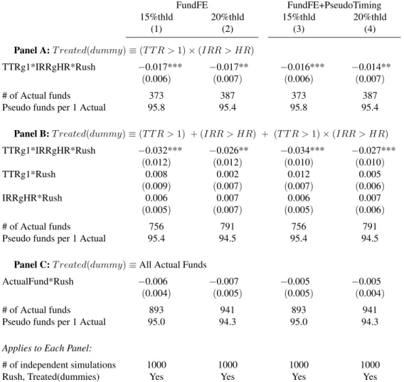
In one set of tests, the control group includes all funds that did not meet the criteria of
Informed GP which means that upon reaching the threshold X% they either (a) did not have
a positive track record of market-timing, or (b) the fund to-date performance was below the
hurdle rate. These tests (i) assure that the stopping-time definition based on X-threshold is
not responsible for the results, and (ii) identify the market-timing effect from a
Footprint-on-Firms effect. The estimates are presented in Section 5.5.1. They constitute a comprehensive
17This idea underlies some of the placebo tests discussed in Section 5.5.1.
18Also, fewer funds of relatively recent vintage years reach the threshold.
examination of hypotheses H1 and H2 while identifying GPs market-timing skills from the
effects ofPseudo-timingandFootprint-on-Firms.
Note that forTreated funds,Rushis proportional to carried interest at a very specific time
in a fund’s life – when it is nearly finished cashing in its carried interest. Hence, a comparison
with the effect of control fund Rush times will isolate market-timing from the
Footprint-on-Firms. In other words, theFootprint-on-Firms effect ofRush will be present in both groups,
treatment and control, while the market-timing effect will be in the treatment group only.20
Vintage year fixed effects (in place of group fixed effects) account for exit conditions
vary-ing across funds that are associated with thePseudo-timingalternative (i.e. time-varying risk
premia). I include additional controls in some specifications to address industry-quarter
vari-ation that vintage year fixed effects do not absorb. Conceptually, I need variables with
mar-ket return predictive power to measure the incremental effect of variation in Rush across
In-formed Exits.21 I follow Goyal and Welch (2008) in the return-predictive variables selection,
re-defining variables at industry level where appropriate. The additional controls common
across industries include CAY Ratio of Lettau and Ludvigson (2001), VIX index, U.S.
Trea-sury yields and corporate credit spreads.22 Industry specific controls include price-earnings
and book-to-market ratios de-meaned using the respective 5-year moving average to account
for heterogeneity across industries. Following Ball et al.(2011), I also control for pre-exit
in-dustry returns by including the inin-dustry cumulative excess return versus S&P500 over 5-years
prior to the stopping-quarter.
20In additional tests, I verify that the results are unlikely to be due to the magnitude ofFootprint-on-Firmsbeing cross-sectionally correlated with the treatment assignment by comparingRusheffects in the treatment and control groups in periods different from the stopping-time and considering definition of treatment group that maximize expectedFootprint-on-Firmseffects.
21In arbitrage-free asset-pricing framework, these variables inform about the state of investors marginal utility. Thus, another way to interpret these tests is whether GPs’ timing skills add value once controlling for the variation in investors’ marginal utility.
22It has been shown that much of predictive ability of Lettau-Ludvigson CAY comes from the fact that its construction uses “lookahead (in-sample) estimation regression coefficients”. For example, see Goyal and Welch (2008). To the extentβ estimates continue to hold with and without CAY, the predictive capacity ofRushin
Informed Exitsis orthogonal to the innovations in the U.S. aggregate consumption and income.
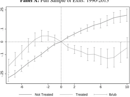
To guard against thePrice Distortionalternative, I examine the reversion of initial returns
following Informed Rush versus those in the control group. Suppose the subsequent returns
were driven purely by a selling pressure, possibly magnified by “copycat” behavior of some
investors tracking PE actions. If this were the case, we would expect the valuations in the
affected industries to rebound as the pressure subsided while the expected deterioration in
the industry fundamentals failed to materialize. Meanwhile, replacing the dependent variable
in model (4.1) with funds’ holding period abnormal returns and breaking T reated into its
skill and incentive components yields a test of H3 corollary. That is, lower holding period
abnormal returns of funds run byinformedGPs without the accrued performance fee incentive
to optimally exit would be consistent with a deviation from the first-best decision (from the
LPs’ stand point).23
4.3.2 Alternative Control Group
As helpful as it can be to identify GP timing skill from Footprint-On-Firms, the control
group comprised of a subset of funds is imperfect. Its limitations originate mainly from two
(conflicting) objectives: (i) likely high false-negative assignment of treatment, (ii) highly
im-balanced fund population over time and industries. It is possible that, conditional on the
as-sumption that exit-Footprintis zero, one can do much better by estimating the market-timing
effect against random exits by the same fund (rather than against actual exits by other funds).
Therefore, in Section 5.5.2 I run additional tests against hypotheticalstopping-timeandRush
-amounts of the sample funds. These tests provide more accurate and robust (i.e. to
Pseudo-timing alternative) estimates of β but, unlike the results with a control group comprised of
actual funds (5.5.1), yield no power to distinguish GPs’ market-timing skill from theFootprint
alternative. They furnish additional insights about hypothesisH2and its corollary, in particular,
allowing for testing of Industry Returnpredictability byRush unconditional on the treatment
assignment.
To conduct these additional tests, I develop a simulation-based estimator that shares much
in common with Simulated Method of Moments, yet better suites this problem.24 In short, I
(i) estimate a model of fund fixed effects for stopping-time and Rush (henceforth auxiliary
model), (ii) independently simulate 1,000 blocks of up to 100 random exits per fund under
this model (henceforth, independent simulations), and (iii) pool Model (4.1) (main model)
estimates over these independent simulations. The estimates that I obtain are not sensitive to
the simulation starting point, are very unlikely to be driven by an ill-specified null hypothesis,
and have good finite-sample properties.25 In Section 5.5.2, I also test hypothesis H3 using a
slight modification of Model (4.1) and a subset of the sample augmented with the simulated
exits. The modification amounts to using standard deviations of pastIndustry Returns as the
dependent variable instead of the future means and restricting the sample of actual fund to
those that lived long enough.
Finally, to determine what drives Informed Rush, GPs’ expectations about industry
cash-flow news or about discount factor innovations, I utilize model 4.1 but swap the future industry
returns withRushas the the dependent variable and instrument the returns with, respectively,
proxies of industry cash-flow news or discount rate news. Such a design allows me to
ad-dress the problem that there are arguably no proxies of, e.g. cash-flow news uncorrelated with
discount-rate news (and visa-verse). Treating the proxy for the other channel as the included
instrument enables me to better absorb the unrelated variation while making sure that the
chan-nel of interest is, in fact, correlates withRush tightly enough. These tests are implementable
using both types of control exits: those of other funds and the simulated ones for the treated
funds. Section 5.5.3 has the results and further details.
In summary, my key identifying assumption is that the alternative explanations to the timing
24Section 5.5.2 and A.2 provide further details, discussion as well as robustness and falsification tests.
25See Appendix A.8.