Estimating Personalized Diagnostic Rules Depending on
Individualized Characteristics
Ying Liu*, Yuanjia Wang*, Chaorui Huang**, and Donglin Zeng†
*Department of Biostatistics, Mailman School of Public Health, Columbia University
**Brain and Mind Research Institute, Weill Cornell Medical College, NY, USA
†Department of Biostatistics, University of North Carolina at Chapel Hill
Abstract
There is an increasing demand for personalization of disease screening based on assessment of patient risk and other characteristics. For example, in breast cancer screening, advanced imaging technologies have made it possible to move away from “one-size-fits-all” screening guidelines to targeted risk-based screening for those who are in need. Since diagnostic performance of various imaging modalities may vary across subjects, applying the most accurate modality to the patients who would benefit the most requires personalized strategy. To address these needs, we propose novel machine learning methods to estimate personalized diagnostic rules for medical screening or diagnosis by maximizing a weighted combination of sensitivity and specificity across subgroups of subjects. We first develop methods that can be applied when competing modalities or screening strategies are observed on the same subject (paired design). Next, we present methods for studies where not all subjects receive both modalities (unpaired design). We study theoretical properties including consistency and risk bound of the personalized diagnostic rules, and conduct simulation studies to examine performance of the proposed methods. Lastly, we analyze data collected from a brain imaging study of Parkinson’s disease using positron emission tomography (PET) and diffusion tensor imaging (DTI) with paired and unpaired designs. Our results show that in some cases a personalized modality assignment is estimated to improve empirical AUC compared to a “one-size-fits-all” assignment strategy.
Keywords
Weighted Support Vector Machine; Personalized Screening; Parkinson’s Disease
1. Introduction
Breast cancer screening is one of the most common forms of cancer screening in the United States, where approximately 39 million screening examinations are performed each year [1]. Recently, there is an increasing demand for personalization of breast cancer screening based on assessment of patient risk, consideration of benefit and harm, and patient preferences [2].
HHS Public Access
Author manuscript
Stat Med
. Author manuscript; available in PMC 2018 March 30. Published in final edited form as:Stat Med. 2017 March 30; 36(7): 1099–1117. doi:10.1002/sim.7182.
A
uthor Man
uscr
ipt
A
uthor Man
uscr
ipt
A
uthor Man
uscr
ipt
A
uthor Man
uscr
Although mammography remains the standard screening modality, new imaging
technologies such as breast magnetic resonance imaging (MRI) may be more sensitive for some women with smaller lesion size and/or with denser breasts [3]. Similarly, recent research in prostate cancer has led the US Preventive Services Task Force to recommend prostate-specific antigen (PSA) screening in high risk population instead of the general population [4]. To formally study personalized screening strategies, initiatives such as the Population-based Research Optimizing Screening through Personalized Regimens (PROSPR) examine how to improve screening process by tailoring based on risk, imaging modalities, and preferences [5].
Besides the potential of personalization in cancer screening, there is also a demand for personalized screening in other medical fields such as mental disorders and neurological disorders. For example, with advances in neurobiology, the current National Institute of Mental Health (NIMH) Strategic Plan calls for the development of new ways of classifying psychopathology and mental disorders based on dimensions of observable behavior and biological measures [6, 7]. Brain imaging biomarkers provide an important source of information in addition to clinical symptoms to assist assessments of of mental disorders, although the science of using neuroimaging techniques to diagnose psychiatric conditions is in an early stage [6, 8]. For neurological disorders, some imaging studies have demonstrated group differences between patients and matched controls [9, 10]. Given that patient
heterogeneity is commonly observed, it is conceivable that some imaging biomarkers may be more sensitive in certain subgroups of patients at different stage of disease progression. However, little work has been done to make personalized selection of imaging modalities, which could potentially improve diagnostic accuracy.
Parametric or semiparametric statistical methods have been developed in the literature to examine heterogeneity in the performance of medical tests and to combine tests to make diagnosis. For example, there are three approaches to compare various tests [11]: empirical methods, distribution modeling methods and distribution-free parametric methods [12, 13]. It is rare that a single biomarker can achieve adequate diagnostic accuracy, and there is a need to create composite measures by combining potentially large number of markers. These methods encounter challenges when the number of biomarkers increases. Some other relevant work aiming at identifying optimal combination of diagnostic markers include maximum-likelihood estimators based on generalized linear models or nonparametric models [14, 15]. However, their focus is on improving the overall performance of the combined test applied to the entire sample under a uniform strategy that administers the same test to all individuals.
An approach to achieve crude personalization when administering a diagnostic test is to compare the area under the receiver operating characteristic (ROC) curve for various testing modalities across subgroups. However, it is often unknown how to define subgroups, and thus the number of subgroups to be examined in an exploratory analysis increases exponentially. As a result, such an approach is subject to penalization by multiple comparisons, and thus cannot accommodate high-dimensional imaging measures or other biomarkers. Several recent work proposed machine learning methods to estimate
personalized treatment regimens from data collected in multi-stage clinical trials [16, 17].
A
uthor Man
uscr
ipt
A
uthor Man
uscr
ipt
A
uthor Man
uscr
ipt
A
uthor Man
uscr
The advantages of machine learning methods include minimal assumptions on the underlying data structure distribution and computational feasibility to handle high-dimensional feature variables with moderate sample size. However, there has been little discussion on machine learning methods for studying personalized medical diagnosis and screening, despite the clear clinical needs.
The goal of this paper is to develop a data-driven machine learning method to determine the best diagnostic rule to assist personalized recommendation for screening and diagnostic practices. We propose to estimate the optimal screening rule depending on subject-specific characteristics to maximize a weighted combination of sensitivity and specificity. We show that identifying the optimal diagnostic rule is equivalent to a weighted classification problem. The estimated diagnostic rule automatically chooses between two competing modalities for each subject to maximize the performance and is guaranteed to perform at least as good as assigning the same modality to all subjects (one-size-fits-all rule). Paired and unpaired designs are considered: in a paired design, both competing modalities are administered to all subjects; by contrast, each subject receive only one modality in an unpaired design. The method can easily handle high-dimensional feature variables and incorporate flexible non-linearity and correlation among variables. Theoretical properties including consistency and risk bound are shown. Simulation studies demonstrate that the proposed method can improve the empirical area under the receiver operating curve (AUC). Lastly, we analyze data collected from a brain imaging study of Parkinson’s disease (PD) using Fludeoxyglucose Positron Emission Tomography (FDG-PET) and Diffusion Tensor Imaging - Structural Magnetic Resonance Imaging (DTI-MRI) under paired and unpaired designs. We show that a personalized modality assignment rule can improve the empirical AUC compared to a “one-size-fits-all” strategy and gain clinical insights.
2. Methods
2.1. Personalized diagnostic rules and performance measure
Consider a dichotomous disease outcome (D = 1: diseased and D = 0: non-diseased) and two diagnostic modalities or screening procedures (A versus B). Let X denote a vector of subject-specific characteristics including a subject’s risk factors or prognostic biomarkers. Our goal is to derive a decision rule to recommend one diagnostic modality depending on X such that for patients with feature variables X, sensitivity of the recommended modality is not lower than the alternative modality; while for healthy control subjects with the same feature variables X, specificity of the recommended modality is also not lower than the competing modality.
Diagnostic tests are often ordinal or dimensional measures. For example, in cancer screening studies, radiologists assess an image obtained from certain imaging modality and assign a diagnostic score to describe the likelihood of a subject having a benign or malignant test result. For breast cancer screening, the malignancy likelihood score, BI-RADS [18], is obtained from breast imaging studies where a radiologist rates a mammogram or other image into a BI-RADS score ranging from 0 to 6 (0: Incomplete, 1: Negative, 2: Benign finding, 3: Probably benign, 4: Suspicious abnormality, biopsy recommended, 5: Highly
A
uthor Man
uscr
ipt
A
uthor Man
uscr
ipt
A
uthor Man
uscr
ipt
A
uthor Man
uscr
suggestive of malignancy, biopsy recommended, 6: Known biopsy, proven malignancy). For neuropsychiatric disorders, biomarkres are explored to assist disease diagnosis [19, 7].
Denote YA as the diagnostic score rated using modality A and YB rated using modality B. Assume that YA and YB are rated on a common scale and a higher score is associated with greater likelihood of being diseased (or malignant). In a paired design, both diagnostic scores YA and YB are observed for each subject. Let (X) denote a screening rule
determining the choice of modality A or B depending on the subject-specific characteristics, X, where (X) = 1 indicates choosing modality A and (X) = −1 indicates choosing modality B. That is, (·) maps X to {1, −1}. Note that a more sensitive modality will lead to a higher screening score for diseased subjects and a more specific modality will lead to a lower screening score for non-diseased subjects. Thus for diseased subjects, if YA > YB we expect an effective rule to assign (X) = 1 for high sensitivity; and if YA < YB, we expect
(X) = −1. Equivalently, a desirable should yield a large value of
to achieve high sensitivity. Similarly, for non-diseased subjects, a desirable will yield a large value of
to achieve high specificity. To consider both sensitivity and specificity when estimating , introduce ω0 as a pre-specified weight in [0, 1] to balance the above two objectives with a default of ω0 = 0.5 if none is preferred. The goal for finding an optimal personalized diagnostic rule is then to solve an optimization problem:
(1)
One potential limitation of this objective function is that the derived rule does not
differentiate between subjects with YA much larger than YB from subjects with only slightly greater YA compared to YB. A solution is to incorporate the difference between diagnostic scores under two modalities into the classification rule in (1). Specifically, define Z = |YA − YB| and we aim to solve the following objective function
(2)
A
uthor Man
uscr
ipt
A
uthor Man
uscr
ipt
A
uthor Man
uscr
ipt
A
uthor Man
uscr
Since I(−1 ≠ (X)) = 1 − I(1 ≠ (X)), criterion (1) and (2) can be unified as
(3)
where W = ωD + (1 − ω)(1 − D) for (1) and W = [ωD + (1 − ω)(1 − D)]Z for (2). Here, ω = (ω0/p)/[ω0/p + (1 − ω0)/(1 − p)], where p is the disease prevalence. The decision rule that minimizes (3) is referred as the optimal personalized diagnostic rule, which we denote as *. In the following sections, we will propose methods to estimate * under paired and
unpaired design.
2.2. Estimation under a paired design
When diagnostic tests do not interfere with each other and when feasible, paired design [11] where each subject is administered with both tests is used. Paired design minimizes between subjects variation in the estimation and eliminates the possibility of confounding. Therefore it provides more efficient assessment and valid comparison of the performance of each test. Specifically, in a paired diagnostic study, patients and controls are recruited and each subject receives two diagnostic modalities (or diagnostic tests), Ai and Bi. Radiologists blinded to the disease status give rating scores (e.g. BIRADS scores), YAi and YBi, respectively, to assess the likelihood of a disease (or malignancy). An empirical version of the minimization problem (3) based on n samples becomes
(4)
where Wi = ωDi + (1 − ω)(1 − Di) for (1), Wi = [ωDi + (1 − ω)(1 − Di)]Zi for (2), and Zi = | YAi − YBi|.
Direct minimization of (4) is a difficult problem due to the discontinuity of the indicator function. However, the objective function in (4) is in fact the empirical weighted misclassification error rate in a classification problem treating Vi as class labels, Xi as feature variables, and each subject being weighted by Wi. Many machine learning
techniques can be applied to find the optimal rule *. Particularly, we choose large margin classifiers due to their successful applications in many fields. Let f(x) be a diagnostic decision function associated with the classification rule , i.e., (x) = sign(f(x)), and define ℒ(υ f) as a large margin-based loss function, for example, hinge loss ℒ(υ f) = (1 − υ f)+ that is associated with Support Vector Machine (SVM) classifier [20, 21]. We propose to estimate the unknown decision function f via the minimization problem:
(5)
A
uthor Man
uscr
ipt
A
uthor Man
uscr
ipt
A
uthor Man
uscr
ipt
A
uthor Man
uscr
where λn is a pre-specified tuning parameter, ℋ is a normed space to which f belongs, and || f||ℋ is the norm or the semi-norm defined in ℋ. Examples of ℋ include a linear space consisting of α + βT x and ||f||ℋ is the Euclidean norm of β, or a reproducing kernel Hilbert space (RKHS) [22, 23] based on some kernel function K(·, ·), and ||f||ℋ is the norm defined in this RKHS.
The optimization problem in (5) can be carried out via its dual problem. Following the KKT condition [24], one can easily show that its dual problem is
(6)
subject to constraints 0 ≤ αi ≤ Cn Wi, i = 1, …, n and , where Cn is the tuning parameter and Cn = 1/λn ([21], page 426). Here,< Xi, Xj > is the inner product defined in the
space ℋ: if ℋ consists of linear function, then ; if ℋ is the RKHS embedded with kernel function K(·, ·), then < Xi, Xj >= K(Xi, Xj). For the latter, the most
commonly used kernel function is the Gaussian kernel where
and 1/σn is the bandwidth tuned using data. Here, we use the notation from [25] and σn is the reciprocal of the tuning parameter in traditional Gaussian kernel function. Because the optimization (6) only involves the inner product of Xi and Xj, the computational cost is related to the sample size n instead of the dimensionality of X. Thus, the
high-dimensionality of X does not cause computational difficulties in the kernel-based method once the distance is defined. Computationally, (6) can be solved by quadratic programming algorithms, and the tuning parameter Cn is selected using cross-validation across a grid 2−15, 2−14, …, 214, 215.
When there are multiple radiologists providing rating scores for each modality, a simple method to incorporate results from multiple readers is to consider the average performance over the readers. That is, we solve the following problem to derive the personalized diagnostic rule:
where N is the number of readers and Wik and Vik are the corresponding weights and class labels defined for each subject i and reader k.
2.3. Estimation under an unpaired design
In many other diagnostic studies, subjects may not undergo multiple modalities due to interference, tests having significant risk, high cost, or simply non-feasible [11]. In these cases, an unpaired design, where one group of subjects receive diagnostic modality A and the other matched group of subjects receive diagnostic modality B, is used. Under an
A
uthor Man
uscr
ipt
A
uthor Man
uscr
ipt
A
uthor Man
uscr
ipt
A
uthor Man
uscr
unpaired design, directly comparing the diagnostic performance of A and B on the same subject is no longer feasible. Since subjects may receive only one of the two modalities, we introduce random variable M to denote the modality that the subject actually receives, where M = 1 indicates receiving A and M = −1 indicates receiving B. Let Y be the observed rating score which is YA if M = 1 and YB if M = −1. Since in an unpaired design each subject has only one outcome (YA or YB) observed, the minimization in (3) cannot be directly
implemented using the observed data. To estimate the optimal personalized diagnostic rules using the unpaired data, we require missing at random (MAR) condition, (C.1): YA, YB and M are independent given X and D. The implication of (C.1) is that a subject’s modality assignment M in a diagnostic study is conditionally independent of their missing rating score given their observed feature variables X, disease status, and observed rating score. This condition also assumes that the dependence among patient’s observed and unobserved rating scores YA and YB must be fully explained by X and D. The MAR assumption (C.1) is necessary when borrowing other similar subjects’ diagnostic scores to infer a particular subject’s missing rating score on modality A or B.
To estimate (3), we use similar pairs of subjects where one receives modality A but the other receives B to approximate the terms in (3). Select a diseased subject (D = 1) who is tested by modality A and has feature variables X and rating score YA. Select another independent diseased subject (D̃ = 1) who is tested by modality B and has feature variables X̃ and rating score ỸB. If X and X̃ are close, under condition (C.1) we expect a desirable decision rule should assign the first subject to A if rating scores YA ≥ ỸB, and to B if rating scores YA < ỸB. Similarly, for a pair of non-diseased subjects, a desirable decision rule will choose the modality with rating scores YA ≤ ỸB. The similarity between two subjects is characterized using kernel distance kan (||X − X̃||) where kan (·) is a kernel function with bandwidth an. In our simulation studies and real data analysis, an is chosen so that the pairs of samples with distance less than an is fixed to be a non-small portion of pairs (for example, 15% to 30%). Cross-validation can also be used to choose an with additional computational cost.
Furthermore, since subjects may receive A or B with different probability since the modality is not randomized, we adjust for this propensity by inverse probability weighting, where we denote π(X, D) as the probability of M = 1 (receiving modality A) given X and D.
Subsequently, for pairs of diseased subjects, a desirable decision rule (·) will yield a large value of
Similarly, for non-diseased pairs a desirable rule will lead to a large value of
As in a paired design, introducing ω0 as a weight for balancing sensitivity and specificity, we aim to maximize a weighted summation of the above two terms. Furthermore, to
A
uthor Man
uscr
ipt
A
uthor Man
uscr
ipt
A
uthor Man
uscr
ipt
A
uthor Man
uscr
incorporate the difference of the observed scores, we can include the magnitude of |YA − ỸB| in the above expectation and define weights ω as in the paired design.
To summarize, we maximize
(7)
where O = (YA, X, D), Õ = (ỸB, X̃, D̃), O and Õ are independent. Note here
and Q(O, Õ) = ωD + (1 − ω)(1 − D) if one does not weight by the difference on observed scores, while Q(O, Õ) = |YA − ỸB|{ωD + (1 − ω)(1 − D)} if one does. To see how (7) approximates (3), we note
where the last step uses the MAR assumption in (C.1). Moreover, when an converges to zero, the last term approximates the following quantity up to some constant
which is equivalent to
This follows by the conditional independence of YA and YB given (X, D) and the fact that ỸB is an independent copy of YB. Note that Q((YA, X, D), (YB, X, D)) = ωD + (1 − ω)(1 − D), if one does not weight by |YA − YB|; and it is Q((YA, X, D), (YB, X, D)) = |YA − YB| {ωD + (1 − ω)(1 − D)}, if one does. By the definition of W in Section 2.1, the maximization becomes
A
uthor Man
uscr
ipt
A
uthor Man
uscr
ipt
A
uthor Man
uscr
ipt
A
uthor Man
uscr
which is exactly the same optimization problem as in (3). This justifies using (7) to find the optimal diagnostic rule.
Using data collected in an unpaired study, we can maximize the empirical version of (7), which is given as
where Vij = (2Di − 1)(2I(Mi = 1) − 1)sign(Yi − Yj), and p̂(M, X, D) is an estimator of p(M, X, D) by regressing M on (X, D). These propensity scores are obtained by logistic regression or other machine learning approaches. Again, due to the difficulty of optimization involving an indicator function (zero-one loss), one can replace it by a large-margin based loss function ℒ(·) as:
(8)
Similar to the paired design case, weighted support vector machine can be used to find the best rule *(x) when ℒ(·) is the hinge loss.
3. Theoretical Properties
In this section, we provide theoretical justification of the proposed optimal rule. We denote the expression (3), E[WI(V ≠ (X))], as ℛ(f) when (X) = sign(f(X)). Since
it is easy to see that the Bayes decision rule is given by
We further define Rℒ(f) = E[Wℒ(V f(X))] for a large margin loss ℒ(·). Then it is clear that our estimated rule minimizes the empirical version of Rℒ(f) for the paired design and minimize an approximated empirical version of Rℒ(f) in the unpaired design. Therefore, it is natural to ask whether the minimizer of Rℒ(f) also minimizes ℛ(f). Our first theorem gives this Fisher consistency and compares the approximation error due to using Rℒ(f).
A
uthor Man
uscr
ipt
A
uthor Man
uscr
ipt
A
uthor Man
uscr
ipt
A
uthor Man
uscr
Theorem 1
If f̃ minimizes Rℒ(f), then *(x) = sign(f̃ (x)). Furthermore, for any f,
The proof of Theorem 1 follows from Proposition 3.1 and Theorem 3.2 in [26] by treating V as the treatment assignment in their context, and thus omitted here.
Our next two theorems provide convergence rates for ℛ(f̂) − ℛ(f*), where f̂ is the estimated decision function by minimizing (5) for the paired design and (8) for the unpaired design when ℒ(z) = (1 − z)+ and ℋ is chosen to be the RKHS associated with the Gaussian kernel with bandwidth 1/σn. The particular choice of ℋ is due to the fact that any L2-integral function can be well approximated by the function in ℋ if σn is chosen to be large enough [25]. To state the convergence rate, we need the so-called geometric noise assumption for the probability distribution (W, V, X), which assumes that there exists a constant C > 0 such that
where q is a constant in (0, ∞), d is the dimension of X, and Δ(x) is the distance of x to the region {x′ : f(x)f(x′) < 0}. This condition is used in [25] to derive the convergence property for the support vector machine. Some examples of q are given in [25]. Our next Theorem 2 gives the asymptotic property of f̂ for the paired design.
Theorem 2
In a paired design, let f̂ minimize (5) in ℋ. Suppose . Then for any δ > 0, 0 < ν < 2, there exists a constant c(ν, δ, d) such that
where with c1 = 2/(2 + ν) + (2 −
ν)(1 + δ)/[(2 + ν)(1 + q)]. Furthermore, if we choose λn = n−c2 where c
2 = 2(1+q)/([(4 + ν)q + 2 + (2 − ν)(1 + δ)], then ℛ(f̂n) − R* = O
p(n−c2q/(1+q)).
Theorem 2 shows that with proper choice of the bandwidth for the Gaussian kernel for ℋ, the convergence rate of the risk for f̂n, as compared to the Bayes risk, is of a polynomial order in n. The proof Theorem 2 follows exactly the same arguments as proving Theorem 3.4 in [26], where their R is equivalent to our W and their A is equivalent to our V. Thus we skip the proof.
We now consider the unpaired design. We note the difference between (8) and (5) is the kernel approximation
A
uthor Man
uscr
ipt
A
uthor Man
uscr
ipt
A
uthor Man
uscr
ipt
A
uthor Man
uscr
Then f̂, which minimizes (8), minimizes
where Pn denotes the empirical measure. Thus, to establish the convergence rate of ℛ(f̂), it is necessary to examine the approximation of ĝ(O, M; f) to Wℒ(V f) which depends on the kernel approximation using kan (·). This gives the following theorem.
Theorem 3
Under the same conditions in Theorem 2 and the same choices of λn and σn, if we further assume the conditional density of X given (M, D, Y ) is twice-continuously differentiable
and with k(·) being a kernel function symmetric with respect to 0, furthermore, supO |p̂(M, X, D) − p(M, X, D)| = Op(n−γ) for some γ > 0 and inf(M, X, D) p(M, X, D) > 0, then it holds
where c2 is a constant depending on (q, ν, δ).
The condition regarding p̂(M, X, D) in Theorem 3 concerns with the accuracy in estimating the propensity score. Particularly, if a parametric model is used to estimate p(M, X, D) consistently, it is clear γ = 1/2. Proof of Theorem 3 is provided in the Web Appendix A.
4. Numeric Studies
4.1. Simulations Under Paired Design
In a paired design, we observe both modalities A and B for all the subjects. We simulate a sample size of 100 subjects (n = 100), half of the subjects are diseased (Di = 1) and the other half are non-diseased (Di = 0). For each subject i with disease status Di = d, we generate Xi = (X1i, …, Xpi) from a uniform distribution on [0, 1]. We generate underlying continuous rating scores for modality A and B as
where (εAi, εBi) follows a bivariate normal distribution with mean zero, and we consider two cases for the covariance matrix of error terms for ỸA and ỸB: (1) independent case where
A
uthor Man
uscr
ipt
A
uthor Man
uscr
ipt
A
uthor Man
uscr
ipt
A
uthor Man
uscr
so that assumption C.1 holds; and (2) correlated case where
as a sensitivity analysis. Next, to imitate real studies we obtain observed discrete rating scores as
Then we apply the proposed methods to determine the optimal personalized diagnostic rules.
We compare a few methods of modality assignment in terms of their ROC curves and AUC. The first two are “one-size-fits-all” rules where all subjects receive modality A or all subjects receive modality B. The next one is to estimate the optimal personalized rule depending on a subject’s covariates X without weighting by the magnitude of the difference of the rating scores on A and B,
The last method is to estimate the optimal personalized rule accounting for the magnitude of the difference of the rating scores:
We compare ROCs and AUCs produced by different methods based on 100 replications. In all simulation settings, we used an independent testing data set of 10, 000 samples to compute ROCs and AUCs. Specifically, for each cut point on the grid of (1, 2, 3, 4, 5, 6), we computed sensitivity and specificity of the estimated optimal modality and obtained the ROC and AUC. The tuning parameter Cn was chosen by cross validation across grid points of 2−15, 2−14, …, 214, 215.
In Table 1 and Figure 1, we report the results comparing diagnostic performance of four methods: (a) all receives modality A; (b) all receives modality B; (c) each subject receives modality chosen by wSVM1; and (d) each subject receives modality chosen by wSVM2. Table 1 summarizes the empirical AUCs and standard deviations across 100 replications of analyses (a) through (d) under several choices of ω and Figure 1 shows the average ROC curve. The proposed personalized diagnostic rule method performs similarly regardless of whether condition (C.1) holds or not (independent rating scores or correlated scores). When ω = 0.5 and 0.75, wSVM1 and wSVM2 increased the empirical AUC by about 5%.
Although the average ROC curve of modality A and B are quite close, using ω = 0.5 or 0.75, the proposed optimal personalized rule assigning modality according to subject-specific covariates improves sensitivity and specificity at all thresholds compared to assigning all subjects to either A or B. Comparing wSVM1 and wSVM2, they have similar performance
A
uthor Man
uscr
ipt
A
uthor Man
uscr
ipt
A
uthor Man
uscr
ipt
A
uthor Man
uscr
except for ω = 0.25. In practice, the choice of ω depends on the relative importance of sensitivity and specificity in the target population where the diagnostic tool will be used. If no such prior information is available, a common choice is ω = 0.5.
Additional simulation results of unpaired design are provided in the Web Appendix B, where the results are similar to the paired design. We also provide a sensitivity analysis of violation of MAR for the unpaired analysis in Appendix D.
4.2. Simulation 2: a Breast Cancer Study
In this setting, we imitate a breast cancer screening study with paired modality measures [3], where we compare mammography with the combined screening using both mammography and MRI. Several covariates are considered: X1 is a subject’s age where older age is associated with a greater risk for breast cancer; X2 is BRCA1 or BRCA2 mutation status where carriers of either mutation will have a greater risk; X3 is the density of breast where it is more difficult for mammography alone to detect tumor for denser breasts. Age, mutation status and breast density are observed subject-specific covariates. In our simulation settings, we simulate MRI to be more sensitive to detect smaller tumor, and mammography to have the same sensitivity but higher specificity for larger tumor. To be more realistic, we also simulated tumor size (X4) as an additional unobserved variable to be associated with breast cancer risk but not available at the screening stage without biopsy, and we assumed X4 to be increasing with age. In this simulation scenario, all covariates X1 through X4 influence a radiologist’s ability to rate a tumor sample. Detailed simulation scheme and empirical AUC are provided in the Web Appendix C.
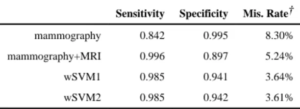
We compare ROCs and AUCs produced by different methods on an independent test set of 10, 000 subjects and repeated simulations 100 times similar to the previous setting. Sensitivity, specificity and classification accuracy are presented in Table 2. Using mammography alone on all subjects leads to a lower sensitivity (84.2%) and higher specificity (99.5%), and combining mammography and MRI increases the sensitivity to 99.6% with a reduced specificity of 89.7%. The personalized assignment of modality (either mammography alone or combined) using our proposed method wSVM1 and wSVM2 increases the sensitivity to be close to modality B (98.5%) without sacrificing the specificity (94.1% and 94.2%). Thus, wSVM1 and wSVM2 reduce the overall miss-classification rate from 8.30% for mammography alone and 5.24% for mammography and MRI combined to 3.64% and 3.61%, respectively.
To demonstrate the interpretability of our proposed method, the linear rule estimated in one replication is f(X) = 1.21 − 0.47 X1 − 0.38 X2 − 0.97 X3 for wSVM1 and f(X) = 1.23 − 0.43 X1 − 0.33 X2 − 0.98 X3 for wSVM2. The fitted rule recommends the more sensitive combined test of MRI and mammography to older subjects with the BRCA1 or BRCA2 mutation due to their higher risk of breast cancer. The negative coefficient for X3 suggests subjects with denser breast tissues are more likely to benefit from the combined test since the tumors may be harder to be detected using mammography alone. In contrast, for younger subjects without the BRCA mutations and with thinner breast tissues, using mammography alone may be optimal.
A
uthor Man
uscr
ipt
A
uthor Man
uscr
ipt
A
uthor Man
uscr
ipt
A
uthor Man
uscr
5. Real Data Example: a Parkinson’s Disease Study
In this section, we analyze data collected from a Parkinson’s disease (PD) imaging study [27]. PD is a disabling neurodegenerative disorder diagnosed on the basis of cardinal motor features, including asymmetric bradykinesia, rigidity, and tremor [28]. In addition to motor impairment, clinically important non-motor symptoms such as anxiety, depression, apathy, and cognitive dysfunction frequently occur and have a major impact on quality of life [29]. Recent research on PD diagnosis is shifting from relying on clinical symptoms to predicting PD at risk status before onset of clinical symptoms using biomarkers [30]. There has been considerable interest in evaluating the potential of advanced non-invasive neuroimaging techniques, such as positron emission computed tomography (PET), and magnetic resonance imaging (MRI) to provide objective measures of dysfunction in PD, thereby enabling accurate diagnosis, predicting disease onset, and monitoring disease progression [9]. Previous study revealed a specific metabolic pattern that was associated with the diagnosis of PD from [18F]-fluorodeoxyglucose (FDG)-PET images, which involved significant elevated brain metabolism in bilateral posterior lentiform nucleus and posterior cingulate, and metabolic reductions in bilateral temporo-parietal association cortex in PD as compared to matched controls [27]. In addition, diffusion tensor imaging (DTI) MRI showed
significantly increased mean diffusivity (MD) values in the posterior cingulate and
decreased fractional anisotropy (FA) values in the white matter, which were both associated with memory deficits in PD, as assessed by California Verbal Learning Test.
Given the heterogeneous nature of PD and the fact that the course of disease progression varies among different individuals, it is important to develop methods for personalized recommendation to assist diagnosis of PD based on individual risk factors. Our proposed methods are used to explore whether there are subgroups of PD patients whose measures from FDG-PET might be a better screening marker compared with DTI. Imaging examinations and neuropsychological assessments for each participant were completed within a one-month time period. Imaging of PD subjects was performed in the practically-defined off state, after antiparkinsonian medications had been withheld for 12 hours. Subjects with PD underwent a full Unified Parkinsons Disease Rating Scale (UPDRS) [31] examination performed by a neurologist. Mood and behavior were measured in terms of depressive symptoms with the Beck Depression Inventory-II [32]. The diagnosis of PD was made according to United Kingdom Brain Bank criteria [33].
In our analysis, subject-specific covariates being considered include BDI score for depression, BAI score for anxiety, UPDRS motor symptoms categorized at 50%th, 75%th and 90%th quartiles, and demographic variables such as age, gender, and years of education. All feature variables were standardized before applying the proposed methods. One
requirement for applying wSVM is that YA and YB are on the same scale and thus
comparable. In the PD study, the imaging measures may not be on the same scale. Thus, we considered a rank-based measure by using percentiles obtained from the empirical
distribution functions for each subject as YA and YB. Similar procedure is used in [34] to compare biomarkers measured on the different scales. Our analysis sample includes both paired and unpaired data. There are 32 patients (19 cases and 13 controls) on whom both image modalities were measured and with no missing data on the feature variables. There
A
uthor Man
uscr
ipt
A
uthor Man
uscr
ipt
A
uthor Man
uscr
ipt
A
uthor Man
uscr
are 34 subjects who have only one modality, where 16 subjects (7 cases) have only MRI measures, and 18 subjects (11 cases) have only PET measures. To compare different methods, we used “leave-one-out” cross validation to compute AUC: for each subject, we used all other subjects as the training data set, and predicted the optimal modality for this subject; we then pooled all these “validation” data to calculate the AUCs using those subjects whose actual modalities were the same as the optimal modalities.
We first show the results for paired data. We compare fractional anisotropy (FA) in white matter and metabolic rate in the parietal lope (PAR). For two one-size-fits-all rules, the empirical AUC is 89.9% if using FA as a PD diagnostic measure on all subjects and 71.7% if using PAR, indicating FA is preferable. To fit a personalized diagnostic rule, we examine both weighted and unweighted schemes. Considering all 7 aforementioned covariates, wSVM2 chooses FA as the better screening modality for all subjects and gives the empirical AUC of 89.9%, while wSVM1 choose FA for all but 2 subjects, and gives an empirical AUC of 88.1%. If excluding UPDRS, both wSVM schemes will choose the superior screening method, FA, for all subjects. The ROC curves are shown in Figure 2a. In terms of the fitted diagnostic function, the intercepts for wSVM1 is 0.29, and 0.22 for wSVM2, and the coefficients for the feature variables are negligible (on the scale of 10−5), indicating none of the feature variables distinguishes the diagnostic ability between FA and PAR, and thus there is no clear subgroup for which one modality outperforms the other. In this paired data analysis, we demonstrated that when there is a universally superior modality (in this case, FA) and no subgroup for which the alternative modality improves performance can be found, the proposed method will choose the modality with superior performance.
Next, we show results of unpaired analysis. Here we compare the mean diffusivity (MD) measure in the posterior cingulate obtained from DTI-MRI and metabolic rate in the lentiform nucleus obtained from FDG-PET. The empirical AUC is presented in Figure 2b. Comparing two one-size-fits-all rules, MD at posterior cingulate on the unpaired sample has an AUC= 87.3% and the metabolic rate at the lentiform nucleus has an AUC= 57.1%. The same feature variables as the paired data analysis are used to fit personalized diagnostic
rules. Here, we used a triangular kernel where , the tuning parameter of bandwidth was chosen to be an = 3 so that there were 90 pairs with none zero kernel weights (i.e., 31% of total number of pairs). We see that wSVM1 estimated a diagnostic rule with a higher AUC than using MD alone (93.7% compared to 87.3%), and wSVM2 achieved an AUC of 85.71%.
The coefficients of the fitted diagnostic rule are presented in Table 3. MD was measured in the posterior cingulate area located at the cingulate cortex. This area is related to emotion and memory. Subjects with higher anxiety score (adjusting for other covariates) may be potentially associated with higher deterioration in posterior cingulate area. Thus, MD measured in this area might be a more sensitive measure for PD patients showing more emotional symptoms (e.g., higher anxiety score). Deterioration in lentiform nucleus is related to motor impairment. For PD patients with more motor symptoms (e.g., with higher UPDRS percentile score) and less anxiety symptoms, metabolic rate at the lentiform nucleus may be a more sensitive measure. In this analysis, we demonstrated that examining
A
uthor Man
uscr
ipt
A
uthor Man
uscr
ipt
A
uthor Man
uscr
ipt
A
uthor Man
uscr
personalized diagnostic rules has the potential to identify subgroups suitable for applying different diagnostic measures, and provides insights on effectiveness of alternative modalities for clinical researchers. Due to the small sample size and exploratory feature of the analyses, a larger study is needed to confirm our findings.
6. Discussion
In this work, we proposed a data-driven approach to estimate optimal personalized diagnostic rule that may depend on subject-specific characteristics such as individual risk factors, biomarkers or subject preference. By drawing a connection with machine learning techniques, the approach can easily handle high-dimensional biomarkers and enjoys robustness of nonparametric decision rules and flexible nonlinear boundaries. The fitted diagnostic rule maximizes a weighted sum of sensitivity and specificity with a user-specified weight. Our theoretical studies examine convergence rate of the fitted decision rule to the true optimal rule. Simulation studies and real data example demonstrate superior
performance of the individualized rules in some cases compared to the “one-size-fits-all” rules where all subjects receive the same modality.
As a note, a similar outcome weighted learning approach has been used in [26] to estimate the best individualized treatment rule among two treatment options according to patient-specific features. Although both papers use weighted SVM for computation, the key difference between this paper and [26] is that our method focuses on selecting personalized rules to optimize diagnostic performance measures, while [26] aims for maximizing reward outcome. Thus, our objective function relates to sensitivity and specificity and depends on direct comparisons of potential outcomes, but this is not the case in [26] which focuses on marginal mean of either potential outcome. Furthermore, data for our analysis can come from very different designs such paired and unpaired as well as multiple readers; but [26] focuses on a single-stage randomized trial design.
In this work, we proposed using the kernel method to approximate the optimization objective (3) for the unpaired design. It relies on the kernel function to measure the
closeness of each pairs. There are situations where the kernel method encounters difficulties: (1) when the dimension of covariates is high; (2) when the types of covariates are mixtures; (3) when the covariates have missing entries. When the dimension of covariate space is high, samples are sparsely distributed in the space, and each sample may not be close to any of its neighbors. Solutions to be considered include using dimension reduction techniques via nonparametric methods (e.g., PCA, slice inverse regression) or semiparametric/parametric models of the performance scores given the covariates (e.g., linear models, single index models), so that a reduced dimensional set of covariates will be included in our approach. Furthermore, variable selection techniques can be incorporated in these procedures to remove non-informative covariates. Challenges also arise when the covariates contain various types (continuous, categorical, binary), one can combine multiple types of distance (e.g., Euclidean distance for continuous covariates, Hamming distance for categorical variables) in the kernel matrix. Lastly, when there are missing values in the covariates, multiple imputation can be used before computing the kernel weights. For the step of
A
uthor Man
uscr
ipt
A
uthor Man
uscr
ipt
A
uthor Man
uscr
ipt
A
uthor Man
uscr
implementing the SVM classifier, one can adopt some imputation based SVM ([21], page 333) to handle the missingness using modified risk function [35].
Our approach here considers maximizing diagnostic performance of a clinical test at the diagnostic stage, which is the first step of the clinical care continuum [36]. When
information at other stages are available (i.e., treatment received) and maximizing long term morbidity or minimizing mortality is the ultimate goal, it is conceivable that a multiple stage decision rule which dynamically determines diagnostic choice and treatment choice can be constructed. Our method can be extended to handle multi-stage personalized rules by a backward induction procedure similar to that used for estimating optimal multi-stage personalized treatment rules [37]. Another interesting extension may be to consider comparing two screening strategies with different timing or frequency, and thus extends the current optimization method from choosing between two modalities to choosing on a continuous scale (timing of screening). Lastly, the proposed methods are illustrated through retrospective case-control diagnostic studies. For prospectively studies, it may be more appropriate to assess positive predictive values (PPV) and negative predictive values (NPV). An extension towards this direction would also be of interest.
References
1. US Food and Drug Administration. Mammography Quality Standards Act and program national statistics 2014. fda.gov/Radiation-EmittingProducts/
MammographyQualityStandardsActandProgram/FacilityScorecard/ucm113858.htm
2. Onega T, Beaber EF, Sprague BL, Barlow WE, Haas JS, Tosteson AND, Schnall M, Armstrong K, Schapira MM, Geller B, et al. Breast cancer screening in an era of personalized regimens. Cancer. 2014
3. Pataky R, Armstrong L, Chia S, Coldman AJ, Kim-Sing C, McGillivray B, Scott J, Wilson CM, Peacock S. Cost-effectiveness of mri for breast cancer screening in brca1/2 mutation carriers. BMC cancer. 2013; 13(1):339. [PubMed: 23837641]
4. Moyer VA. Screening for prostate cancer: Us preventive services task force recommendation statement. Annals of internal medicine. 2012; 157(2):120–134. [PubMed: 22801674] 5. National Cancer Institute. Population-based research optimizing screening. 2011. http://
appliedresearch.cancer.gov/prospr/
6. Fu CH, Mourao-Miranda J, Costafreda SG, Khanna A, Marquand AF, Williams SC, Brammer MJ. Pattern classification of sad facial processing: toward the development of neurobiological markers in depression. Biological psychiatry. 2008; 63(7):656–662. [PubMed: 17949689]
7. Lilienfeld SO. The Research Domain Criteria (RDoC): an analysis of methodological and conceptual challenges. Behaviour research and therapy. 2014; 62:129–139. [PubMed: 25156396] 8. Ecker C, Rocha-Rego V, Johnston P, Mourao-Miranda J, Marquand A, Daly EM, Brammer MJ,
Murphy C, Murphy DG. Investigating the predictive value of whole-brain structural mr scans in autism: a pattern classification approach. Neuroimage. 2010; 49(1):44–56. [PubMed: 19683584] 9. Huang C, Mattis P, Perrine K, Brown N, Dhawan V, Eidelberg D. Metabolic abnormalities
associated with mild cognitive impairment in Parkinson disease. Neurology. 2008; 70(16 Part 2): 1470–1477. [PubMed: 18367705]
10. Huang C, Wahlund LO, Almkvist O, Elehu D, Svensson L, Jonsson T, Winblad B, Julin P. Voxel-and VOI-based analysis of SPECT CBF in relation to clinical Voxel-and psychological heterogeneity of mild cognitive impairment. Neuroimage. 2003; 19(3):1137–1144. [PubMed: 12880839] 11. Pepe, MS. The statistical evaluation of medical tests for classification and prediction. Oxford
University Press; 2003.
A
uthor Man
uscr
ipt
A
uthor Man
uscr
ipt
A
uthor Man
uscr
ipt
A
uthor Man
uscr
12. Metz CE, Herman BA, Shen JH. Maximum likelihood estimation of receiver operating
characteristic (roc) curves from continuously-distributed data. Statistics in medicine. 1998; 17(9): 1033–1053. [PubMed: 9612889]
13. Alonzo TA, Pepe MS. Distribution-free roc analysis using binary regression techniques. Biostatistics. 2002; 3(3):421–432. [PubMed: 12933607]
14. Pepe MS, Cai T, Longton G. Combining predictors for classification using the area under the receiver operating characteristic curve. Biometrics. 2006; 62(1):221–229. [PubMed: 16542249] 15. Wang Y, Chen H, Li R, Duan N, Lewis-Fernández R. Prediction-based structured variable selection
through the receiver operating characteristic curves. Biometrics. 2011; 67(3):896–905. [PubMed: 21175555]
16. Murphy SA. Optimal dynamic treatment regimes. Journal of the Royal Statistical Society: Series B (Statistical Methodology). 2003; 65(2):331–355.
17. Zhao Y, Kosorok MR, Zeng D. Reinforcement learning design for cancer clinical trials. Stat Med. 2009; 28:3294–3315. [PubMed: 19750510]
18. BI-RADS Committee and American College of Radiology. Breast imaging reporting and data system. American College of Radiology; 1998.
19. Dubois B, Feldman HH, Jacova C, Hampel H, Molinuevo JL, Blennow K, DeKosky ST, Gauthier S, Selkoe D, Bateman R, et al. Advancing research diagnostic criteria for Alzheimer’s disease: the IWG-2 criteria. The Lancet Neurology. 2014; 13(6):614–629. [PubMed: 24849862]
20. Cortes C, Vapnik V. Support-vector networks. Machine learning. 1995; 20(3):273–297. 21. Hastie T, Tibshirani R, Friedman J, Franklin J. The elements of statistical learning: data mining,
inference and prediction. The Mathematical Intelligencer. 2005; 27(2):83–85.
22. Aronszajn N. Theory of reproducing kernels. Transactions of the American mathematical society. 1950; 68(3):337–404.
23. Hofmann T, Schölkopf B, Smola AJ. Kernel methods in machine learning. The annals of statistics. 2008:1171–1220.
24. Boyd, S., Vandenberghe, L. Convex optimization. Cambridge university press; 2009.
25. Steinwart I, Scovel C. Fast rates for support vector machines using gaussian kernels. The Annals of Statistics. 2007:575–607.
26. Zhao Y, Zeng D, Rush AJ, Kosorok MR. Estimating individualized treatment rules using outcome weighted learning. Journal of the American Statistical Association. 2012; 107(499):1106–1118. [PubMed: 23630406]
27. Huang C, Dyke J, Voss H, Tsiouris A, Henchcliffe C, Piboolnurak P, Severt L, Ravdin SLNMLD, Maniscalco JS. Multi-modal imaging study of posterior cingulate in parkinsons disease. World Parkinson Congress. 2013
28. Rodriguez-Oroz MC, Jahanshahi M, Krack P, Litvan I, Macias R, Bezard E, Obeso JA. Initial clinical manifestations of parkinson’s disease: features and pathophysiological mechanisms. The Lancet Neurology. 2009; 8(12):1128–1139. [PubMed: 19909911]
29. Emre M. What causes mental dysfunction in parkinson’s disease? Movement disorders. 2003; 18(S6):63–71.
30. Jankovic J, Sherer T. The future of research in parkinson disease. JAMA neurology. 2014
31. Fahn, ERS. the members of the Unified Parkinsons Disease Rating Scale Development Commitee. Recent developments in parkinsons disease. 1987. Unified parkinsons disease rating scale. 32. Beck, AT., Steer, RA., Brown, G. Beck depression inventory. 2. san antonio, tx: the psychological
corporation; 1996. manual
33. Hughes AJ, Daniel SE, Kilford L, Lees AJ. Accuracy of clinical diagnosis of idiopathic
parkinson’s disease: a clinico-pathological study of 100 cases. Journal of Neurology, Neurosurgery & Psychiatry. 1992; 55(3):181–184.
34. Donohue MC, Jacqmin-Gadda H, Le Goff M, Thomas RG, Raman R, Gamst AC, Beckett LA, Jack CR, Weiner MW, Dartigues JF, et al. Estimating long-term multivariate progression from short-term data. Alzheimer’s & Dementia. 2014; 10(5):S400–S410.
35. Pelckmans K, De Brabanter J, Suykens JA, De Moor B. Handling missing values in support vector machine classifiers. Neural Networks. 2005; 18(5):684–692. [PubMed: 16111866]
36. Zapka JG, Taplin SH, Solberg LI, Manos MM. A framework for improving the quality of cancer care the case of breast and cervical cancer screening. Cancer Epidemiology Biomarkers & Prevention. 2003; 12(1):4–13.
37. Zhao Y, Zeng D, Laber E, Kosorok MR. New statistical learning methods for estimating optimal dynamic treatment regimes. Journal of the American Statistical Association. 2014; doi: 10.1080/01621459.2014.937488
38. Hansen BE. Uniform convergence rates for kernel estimation with dependent data. Econometric Theory. 2008; 24(03):726–748.
39. Van Der Vaart, AW., Wellner, JA. Weak Convergence. Springer; 1996.
Appendix A. Proof of Theorem 3
First, from the fact
we have
By the uniform convergence of kernel approximation (c.f., [38]),
. Therefore, we obtain a preliminary upper bound of
which is also an upper bound for the L∞-norm of f̂ by the embedding property of ℋ.
Next, the same proof as Theorem 1 gives
where q(X) is the marginal density of X. Then using the fact that f̂ minimizes (8), we have
Thus, it gives
A
uthor Man
uscr
ipt
A
uthor Man
uscr
ipt
A
uthor Man
uscr
ipt
A
uthor Man
uscr
(A.1)
For the first term in (A.1), we note that ĝ(O,M; f) is Lipschitz continuous in f and according
Theorem 2.1 in [25], the entropy for the unit ball of ℋ is of order . Therefore, using the large deviation results for the empirical process (Theorem 2.14.10, [39]), we conclude that this term is
For the last two terms in (A.1), we again apply the uniform approximation property to ĝ(O,M; f̂) plus the approximation p̂(M,X,D) to obtain
On the other hand, from the condition (C.1), we follow the similar derivation in Section 2 to conclude that
Thus,
Similarly,
Combining these results, we obtain
A
uthor Man
uscr
ipt
A
uthor Man
uscr
ipt
A
uthor Man
uscr
ipt
A
uthor Man
uscr
Theorem 3 thus holds from the choice of λn and σn in Theorem 2.
Appendix B. Simulations Under the Unpaired Design
We simulated covariates Xi, disease status Di and screening scores YAi and YBi under a similar procedure as the paired design in section 4.1. In addition, we created random variable M = 1when modality A is observed and M = −1 when modality B is observed. We
implemented the unpaired algorithm with a triangular kernel . We simulated three scenarios where the modalities were generated following equation 1 and 2. Case 1 and 2 has p = 6 dichotomized variables Xi’s. Here we considered equal weights ω = 0.5. The kernel bandwidth tuning parameter an were chosen to be 1.5 for the binary cases so the the number of pairs with strictly positive weights were around 350 when the sample size is 64, and 1400 when the sample size is 128, which is approximately 30% of the total pairs. Simulation case 3 of the unpaired design considered the same modalities with continuous covariates, where X was generated from a multivariate normal distribution with p = 10. The sample size was n = 100. We considered the same two scenarios for the covariance matrix of error terms for YA and YB, ω = 0.5. The kernel bandwidth tuning parameter an was set to be 1, and there were approximately 350 pairs with non-zero kernel, approximately 15%.
The results are reported in Table B1 and Figure B1. The methods perform similarly for independent modality measurements and correlated modality measurements. Comparing case 1 and 2, we see that the increase of sample size from 6 to 128 greatly improves the performance of the proposed method. In these settings, wSVM2 performs better than wSVM1. For example, in case 2, it improves the empirical AUC by 13%, and we see a large gap between its average ROC curve compared to other three methods. Thus weighting by the magnitude of the difference in two modality screening scores makes a difference in this simulation scenario. Case 3 is a more difficult case, where there are more noise variables, and the covariates are continuous instead of categorical. Our proposed methods wSVM1 and wSVM2 both improve the empirical AUC over “one-size-fits-all” rules by approximately 1% and 4%, respectively.
Table B1
Mean (SD) for Empirical AUC for Unpaired Design Simulation with independent and correlated modality measurements
modality A modality B wSVM1 wSVM2
Independent Correlated Independent Correlated
Case 1 0.739 0.752 0.751(0.026) 0.753(0.027) 0.771(0.05) 0.767(0.047)
Case 2 0.739 0.752 0.765(0.053) 0.761(0.039) 0.834(0.083) 0.838(0.083)
Case 3 0.742 0.745 0.748(0.017) 0.750(0.021) 0.767(0.037) 0.775(0.039)
A
uthor Man
uscr
ipt
A
uthor Man
uscr
ipt
A
uthor Man
uscr
ipt
A
uthor Man
uscr
Figure B1.
Empirical ROC for Unpaired Design Simulation with independent and correlated modality measurements
Appendix C. Details of the Simulation Imitating a Breast Cancer Study in
Section 4.2
Age X1 was simulated from a folded standard normal distribution which is the absolute value of a random variable following standard normal distribution, and BRCA gene type X2 was generated from Bernoulli(0.1). The indicator for disease outcome D was generated from from a logistic model with logit(Pr(D = 1|X) = X1 + X2 − 0.8. For simplicity, we assume the screening outcome of mammography and MRI to be binary indicators of whether
abnormality is detected, which is followed by a decision of whether biopsy should be referred. Modality A represents mammography alone, where YA = 1 denotes the detection of
A
uthor Man
uscr
ipt
A
uthor Man
uscr
ipt
A
uthor Man
uscr
ipt
A
uthor Man
uscr
abnormality under this modality. There were two variables influencing YA are X3 and X4, where density of breast X3 was simulated from a folded normal distribution, and tumor size (X4) was simulated by X4 = 0.3X1 + 0.7e1, with e1 simulated from a folded standard normal distribution. The binary outcome representing detection of abnormality was simulated from
where p is 0.01 + 0.98D − 0.4I(X4 < 0.1)D − 0.4I(X3 > 0.9)D) truncated by [0, 1]. Modality B represents combined mammography and MRI, where YB = 1 represents either
mammography or MRI test detects abnormality, and
The box plot of empirical AUCs of the two proposed methods are presented in Figure C1. We observe a substantial increase in empirical AUC.
Figure C1.
Empirical AUC for Breast Cancer based on n = 1000 and 100 replication
Table D1
Mean and SD of AUC of sensitivity analysis for unpaired modalities
Setting α modality A modality B wSVM1 wSVM2
1 0.5 0.739 0.752 0.749(0.024) 0.775(0.055)
1 1 0.739 0.752 0.751(0.026) 0.767(0.046)
2 0.5 0.739 0.752 0.749(0.022) 0.764(0.044)
2 1 0.739 0.752 0.746(0.028) 0.751(0.029)
A
uthor Man
uscr
ipt
A
uthor Man
uscr
ipt
A
uthor Man
uscr
ipt
A
uthor Man
uscr
Appendix D. Sensitivity Analysis for the Unpaired Design in Simulation
Studies
For the unpaired data we assumed missing at random (MAR), i.e., the choice of modality is independent of the measurement of modality given the observed feature covariates. Here we conducted sensitivity analysis for one simulation setting of unpaired design when this assumption is violated.
We generated data from case 1 in Appendix B with independent covariates. The choice of observed modality was generated depending on the modality measurement from a logistic model. There are two setting of this logistic model, setting 1 is logit(P(M = A|YA, YB)) = αYA + αYB − 6α)); and setting 2 is logit(P(M = A|YA, YB)) = αYA − αYB). The model suggests that the modality assignment may depend on potentially unobserved YA or YB, since in an unpaired design only one modality will be measured. In both settings, we let α take two values, 0.5 and 1. There are 200 replications conducted for each setting and α combination, and the AUC was computed from an independent testing data set of 10, 000 observations. Table D1 presented the mean and SD of the AUC. Our proposed method in three settings shows stable superior performance than one-size-fits-all method. Compared with the results of no violation of MAR in Table B1, where wSVM1 achieves an AUC of 0.751(0.026) and wSVM2 achieves 0.771(0.05), setting 2 is more affected by the violation of MAR assumption when α is large, that is, when the parameters of modality A and B have different signs in the logistic model generating the modality assignment. In this setting, with different signs, the comparative location of center is affected by the violation of MAR. When α has the same sign in setting 1, the result are less affected by the violation of MAR, because the comparative means of two modalities are not shifted by the violation of MAR.
A
uthor Man
uscr
ipt
A
uthor Man
uscr
ipt
A
uthor Man
uscr
ipt
A
uthor Man
uscr
Figure 1.
Average ROC for Paired Design with independent and correlated modality measurements within patients
A
uthor Man
uscr
ipt
A
uthor Man
uscr
ipt
A
uthor Man
uscr
ipt
A
uthor Man
uscr
Figure 2.
ROC curve for brain imaging study for Parkinson’s Diseases
A
uthor Man
uscr
ipt
A
uthor Man
uscr
ipt
A
uthor Man
uscr
ipt
A
uthor Man
uscr
A
uthor Man
uscr
ipt
A
uthor Man
uscr
ipt
A
uthor Man
uscr
ipt
A
uthor Man
uscr
ipt
T
ab
le 1
Mean (SD) for the empirical A
UC for the paired design (with independent and correlated measurements within patients)
ω
modality A
modality B
wSVM1
wSVM2
Independent
Corr
elated
Independent
Corr
elated
0.25
0.692
0.694
0.646(0.044)
0.63(0.046)
0.691(0.015)
0.694(0.013)
0.5
0.692
0.694
0.748(0.047)
0.741(0.048)
0.722(0.040)
0.729(0.046)
0.75
0.692
0.694
0.736(0.044)
0.749(0.048)
0.744(0.049)
A
uthor Man
uscr
ipt
A
uthor Man
uscr
ipt
A
uthor Man
uscr
ipt
A
uthor Man
uscr
ipt
Table 2
Sensitivity and specificity for the breast cancer study simulation
Sensitivity Specificity Mis. Rate†
mammography 0.842 0.995 8.30%
mammography+MRI 0.996 0.897 5.24%
wSVM1 0.985 0.941 3.64%
wSVM2 0.985 0.942 3.61%
†
A
uthor Man
uscr
ipt
A
uthor Man
uscr
ipt
A
uthor Man
uscr
ipt
A
uthor Man
uscr
ipt
T
ab
le 3
Coef
ficients of the f
itted diagnostic rule for the unpaired PD study
Method
Int.
Education
Age
Gender
BDI
B
AI
UPDRS50%
UPDRS75%
UPDRS90%
wSVM1
0.2878
−0.0565
−0.6185
−0.1536
−0.1917
0.8797
−0.0497
−0.1674
0
wSVM2 (×10
−4
)
294.1
−0.18
−0.23
0.33
0.32
0.47
0.26
−0.007