RESEARCH ARTICLE
A confidence predictor for logD using
conformal regression and a support-vector
machine
Maris Lapins, Staffan Arvidsson, Samuel Lampa, Arvid Berg, Wesley Schaal, Jonathan Alvarsson and Ola Spjuth
*Abstract
Lipophilicity is a major determinant of ADMET properties and overall suitability of drug candidates. We have devel-oped large-scale models to predict water–octanol distribution coefficient (logD) for chemical compounds, aiding drug discovery projects. Using ACD/logD data for 1.6 million compounds from the ChEMBL database, models are created and evaluated by a support-vector machine with a linear kernel using conformal prediction methodology, outputting prediction intervals at a specified confidence level. The resulting model shows a predictive ability of Q2=0.973 and with the best performing nonconformity measure having median prediction interval of ±0.39 log units at 80% confidence and ±0.60 log units at 90% confidence. The model is available as an online service via an
OpenAPI interface, a web page with a molecular editor, and we also publish predictive values at 90% confidence level for 91 M PubChem structures in RDF format for download and as an URI resolver service.
Keywords: Conformal prediction, Machine learning, QSAR, Support-vector machine, LogD, RDF
© The Author(s) 2018. This article is distributed under the terms of the Creative Commons Attribution 4.0 International License (http://creativecommons.org/licenses/by/4.0/), which permits unrestricted use, distribution, and reproduction in any medium, provided you give appropriate credit to the original author(s) and the source, provide a link to the Creative Commons license, and indicate if changes were made. The Creative Commons Public Domain Dedication waiver (http://creativecommons.org/ publicdomain/zero/1.0/) applies to the data made available in this article, unless otherwise stated.
Background
Lipophilicity plays a crucial role in determining the phar-macokinetic behavior of drugs. Hydrophilic compounds are typically well-soluble but are likely to exhibit prob-lems with membrane permeability and are more sus-ceptible to renal clearance. Highly lipophilic compounds tend to have low solubility, high plasma protein binding, and they are also more vulnerable to CYP450 metabo-lism. Furthermore, high lipophilicity has been shown to increase the likelihood of target promiscuity and gen-eral toxicity as well as more specific toxicology issues of hERG inhibition, phospholipidosis and CYP450 inhibi-tion [1–3].
From these considerations, it is suggested that optimal ADME properties and the lowest risk for adverse toxic-ity outcomes are expected if a compound’s lipophilictoxic-ity at pH=7.4 lies in a logD range between about 1 and 3
[2] or a logP between 2 and 4 [3]. Several studies indi-cate that these ranges might be even narrower depending
on molecular weight, acid/base properties and/on the desired mode of action of the drug. For example, statis-tical analysis of AstraZeneca Caco-2 membrane per-meability data suggests that the lower limit for passive diffusion is dependent on the molecular weight of com-pounds: a logD>1.7 being required for a 50% chance of high permeability for compounds with molecular weight above 350 Da, logD>3.1 for compounds with molecu-lar weight above 400 Da, and logD>4.5 for compounds with MW above 500 Da [4].
Similarly, analysis of in-house data from Pfizer dem-onstrates that most of the compounds satisfying both cell permeability and in vitro clearance criteria fall into a logD range between 0 and 3 [5]. This study also suggests that higher molecular weight compounds are more con-strained in the range of acceptable logD values; the top of optimum region (referred to as “golden triangle”) peaking to logD of about 1.5 at MW of 500 Da.
Several studies have found that logD or logP of above 3 gives rise to promiscuity and risk for adverse in vivo toxi-cological outcomes [4, 6, 7].
Furthermore, toxicological liabilities such as hERG inhibition depend on the acid/base properties of a drug,
Open Access
*Correspondence: [email protected]
the risk being particularly high for lipophilic bases. For neutral drugs a 30% risk for problematically high levels of hERG inhibition is estimated at logD=3.3 whereas for
basic compounds such risk arises already at logD=1.4 [8].
In a study on CNS drug-likeness, Wager [9] concludes that the most desirable lipophilicity for blood–brain bar-rier penetration is a logD≤2. A logD above 4 is unlikely for a CNS drug.
Taken together, lipophilicity is one of the molecu-lar properties to address in early stages of drug design, to increase chances of selection of compounds that would not fail in development because of poor ADMET characteristics.
Many computational methods to predict logP have been described. Benchmarking of 18 of these methods has shown reasonable results for many of them, with the root mean square error of prediction (RMSEP) for a Pfizer in-house dataset of 96,000 compounds being 0.95 log units for consensus logP and slightly above 1 log unit for best individual algorithms [10]. Prediction of logD is, however, more difficult, as it involves both estimation of logP and estimation of acid and base pKa constants of the compounds, which may introduce further error. Never-theless, AstraZeneca in-house algorithm AZlogD and the commercial ACD/logD algorithm of Advanced Chemis-try Development, Inc. [11] on AstraZeneca an in-house dataset showed a very good RMSEP=0.49 for AZlogD and a reasonable RMSEP=1.3 for ACD/logD [4].
In this study, we present a support-vector machine (SVM) model based on data from 1.6 million compounds in ChEMBL database with logD annotations from the ACD/logD algorithm. The model was distributed as a Docker container and made available as a publicly availa-ble web service exposed with an OpenAPI definition. We evaluated the performance of the model and predicted 91 M compounds from the PubChem database, and made these data available in semantic web format (RDF) for download.
Methods
Data set
ChEMBL is an open, large-scale chemical database con-taining more than 1.7 million distinct compounds with bioactivity data extracted from the chemical literature and calculated molecular properties [12]. From ChEMBL version 23, we extracted all compounds having the cal-culated property acd_logd (calcal-culated logD) at pH=7.4 ,
resulting in 1,679,912 compounds. Standardization of chemical structures was performed by ambitcli version 3.0.2, which is part of AMBIT cheminformatics platform and relies on the CDK library [13–15].
Standardization was performed using default set-tings except for the option ‘splitfragments’ that was set to TRUE. In this way, salt and solvent components were filtered away. After standardization and removal of duplicates the data set consisted of 1,592,127 chemi-cal compounds. To evaluate the predictive ability of the developed models, we set aside a test set compris-ing 100,000 compounds. To perform predictions on the developed model we downloaded 91,498,351 chemi-cal compounds of PubChem database [16], which were standardized in the same way as the compounds from the ChEMBL database.
LogP and logD
The most commonly used measure of lipophilicity is logP, the log of the partition coefficient of a neutral (non-ion-ized) molecule between two immiscible solvents, usu-ally octanol and water. The distribution coefficient, logD, takes into account both the compound’s non-ionized and ionized forms and in the determination of logD the aque-ous phase is adjusted to a specific pH. Most of the drugs and the majority of molecules under research for phar-maceutical purposes do contain ionizable groups, and therefore logD should be used preferentially over logP as the descriptor for lipophilicity, especially when look-ing at compounds that are likely to ionize in physiologi-cal media. Of a particular interest is the logD at pH=7.4
(the physiological pH of blood serum).
Signature molecular descriptor
The compounds were encoded by the signature molecu-lar descriptor [17], generated by CPSign [18]. A signature molecular descriptor constitutes a vector of occurrences of all atom signatures in the dataset, where an atom sig-nature is a canonical representation of the atom’s envi-ronment (i.e., neighboring and next-to neighboring atoms). Signatures distinguish between different atom and bond types, as well as between aromatic and ali-phatic atoms in the atom’s environment. Presence of the same atom signature in several compounds thus indicates that these compounds share identical 2D structural frag-ments. Atom signatures can be calculated up to a prede-fined height (i.e., the number of bonds to the neighboring and next-to neighboring atoms that the signature spans). We here calculated atom signatures of heights one, two and three, which is a set of heights good both for mod-eling as well as for visualization purposes [19, 20].
QSPR modeling by SVM
To model the relationship of logD to the molecular descriptors, we used SVM, a machine learning algorithm that correlates independent variables to the dependent one by means of a linear or nonlinear kernel function. Kernel functions map the data into a high-dimensional space, where correlation is performed based on the struc-tural risk minimization principle; i.e., aiming to increase the generalization ability of a model [21].
We elected to perform correlation by the linear ker-nel using signature molecular descriptors comprised of a vector of 1,068,830 integers. This choice was also sup-ported by results of our earlier, large-scale modeling study, where a linear kernel performed on par with the nonlinear but required dramatically less computational resources [22].
SVM with linear kernel requires fine-tuning of two parameters to obtain an optimal model, namely, the error penalty parameter cost and tolerance of termination cri-terion epsilon. We found optimal cost and epsilon by per-forming grid search with cost values ranging from 0.1 to 10 and epsilon values from 0.1 to 10−5. SVM models were created by the LIBLINEAR software as accessed from CPSign [18, 23].
Conformal prediction
In the conformal prediction framework, conventional single value predictions are complemented with meas-ures of their confidence. In the case of regression, the conformal prediction algorithm outputs a prediction interval around the single prediction point [24]. In QSPR modeling, the size of the prediction interval is deter-mined by some measure of dissimilarity (nonconformity measure) of the new chemical compound to the com-pounds used in the development of the prediction model. Thus, the compound that is “typical” for the data set would more likely be given a smaller interval than a com-pound being in a less explored area or outside the mod-eled chemical domain [25–27].
The size of intervals also depends on the desired con-fidence level (also called validity) which is defined as the ratio of compounds for which the true value falls within the prediction interval. Validity can thus range from 0 to 100%, where 0% means that none of the prediction inter-vals include the true value and 100% means that all of them include the true value.
For inductive conformal prediction, the training set is split into a proper training set and a calibration set. The proper training set is used for creating a predic-tion model and the calibrapredic-tion set is used for comparing new compounds to existing ones and to estimate sizes of intervals for a certain confidence level. The inductive set-ting means that split and training is performed once and
all subsequent predictions are done by the same model; splitting is typically done in such a way that size of cali-bration set is smaller than the size of the proper training set [26].
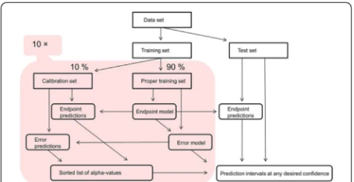
In the present study, we applied a 10-fold cross-confor-mal predictor (CCP) as described in [28]. In brief, this algorithm attempts to reduce the influence of the split into proper and calibration sets by performing multiple such splits, each resulting in an inductive conformal pre-dictor, and aggregating the resulting predictions. Here we chose to use ten aggregated models, and performing the dataset splits in a folded fashion (the cross prefix refers to k-fold cross validation). The workflow of CCP is pre-sented in Fig. 1.
Conformal predictors are always valid under the assumption of exchangeability, i.e., that predicted pounds are drawn from the same distribution as com-pounds used to develop the prediction model. The main criterion when comparing different nonconformity meas-ures is therefore their efficiency, i.e., the sizes of predic-tion intervals in case of regression. Intuitively, a smaller size of prediction intervals indicates a higher efficiency. In this work we evaluated three different nonconformity measures. The simplest measure tested here was based on the prediction error given by the endpoint model, where the nonconformity of compound i, denoted αi is
calculated using Eq. 1. This measure, termed absolute dif-ference, gives the same prediction interval size for all pre-dictions for a given confidence level, but in turn does not require any error model to be fitted and can thus lessen the computational demands.
The second nonconformity measure used, termed nor-malized, assigns larger prediction intervals to objects that are more different from objects used in the model development and hence are “harder” to predict, and smaller intervals to “easier” objects. Naturally, when using normalized nonconformity measures, we expect the median prediction interval to be smaller, i.e., the efficiency to be increased. One of the common ways to obtain a normalized nonconformity measure is by creat-ing an error model, where the dependent variable is the absolute value of error in the endpoint prediction model. This is expected to provide a more efficient nonconform-ity measure than absolute difference, provided that the error model is predictive. The normalized nonconform-ity measure is defined following Eq. 5 in [26], here shown in Eq. 2, where |yi− ˆyi| is the absolute value of error for
object i in the endpoint prediction model and µˆi is the
prediction from an error model (note that both yˆi and µˆi
are calculated when the compound is placed in the cali-bration set, i.e., is not present in the proper training set).
The third nonconformity measure, termed log-normal-ized, proposed in [25], instead of |yi− ˆyi| uses ln|yi− ˆyi|
as dependent variable when fitting the error model. It also introduces a smoothing factor, β, that can be used for “smoothing” the interval sizes, making the small intervals a bit larger and the very large intervals a bit smaller, i.e., reducing the influence of µˆi in calculating αi, Eq. 3. The
smoothing might be advantageous as biological meas-urements always include some measurement errors, pre-cluding predictions with intervals close to 0. Very large intervals, on the other hand, can arise from badly pre-dicted µˆ in the error model. We here created models with β=0 and β=1.
For each of the inductive conformal predictors, αi values
are computed for all compounds in the calibration set and are then sorted in ascending order. When perform-ing a prediction, the test compound is first predicted by the endpoint model to get the prediction midpoint, yˆ.
To compute the prediction interval, the algorithm looks in the ordered set of nonconformity values to to get αconf .lev. , which is dependent on the desired confidence of the prediction. If, for example, we propose that an 80% confidence is required, the αconf .lev. is then the αi value
(2) αi=
|yi− ˆyi| ˆ µi
(3) αi=
|yi− ˆyi|
eµiˆ +β; β≥0
found when traversing 80% of the list. If the nonconform-ity value is dependent on an error model, an error pre-diction, µi, is made. The size of the prediction interval is
then calculated by rearranging the nonconformity meas-ure to solve for |y− ˆy|, resulting in the final prediction interval (yˆ− |y− ˆy|,ˆy+ |y− ˆy|) for the single inductive predictor. The CCP prediction is then computed to be the median prediction midpoint and the median predicted interval size.
Molecule gradient for the prediction
CPSign allows the computation of a “prediction gradi-ent”, as described in [29]. This is managed by altering the number of occurrences of each signature descriptor of the molecule, changing one descriptor at a time. For each alteration a new prediction is made, and the relative change in the prediction output is considered the gradi-ent for that signature descriptor. If the gradigradi-ent value for the descriptor is positive, the altered prediction has given a larger regression value, meaning that adding more of this descriptor would move the prediction to a higher response value, and vice-versa if the gradient value is negative. In CCP, each of the ten models produces its own gradient. The resulting gradient is computed as the median of the individual gradients. The per-descriptor contributions can then be transformed to the per-atom contribution, by summing up all contributions that each atom is part of.
Results and discussion
Development of CCP model
The data set was randomly split into a training set com-prising 1,492,127 compounds and a test set comcom-prising 100,000 compounds. The training set was then used to develop SVM models and the test set was used to fine tune model parameters and assess their predictive per-formance. Optimal model parameters were found by a grid search, starting with a low-complexity model with a low cost for errors, cost=0.001, and a high tolerance for termination criterion, epsilon=0.1. Note that the time required for model development and the model com-plexity increase along with higher cost and lower epsi-lon value. A too low value of cost and/or too high value of epsilon generally results in underfit models with low predictive ability. On the other hand, excessive cost and/ or insufficient epsilon not only make the computations overly time-consuming but also gives rise to a risk for overfitting, indicated by decreasing training set errors but suboptimal predictive performance. As could be expected, the initial model showed low predictive ability, the squared correlation coefficient between acd_logd val-ues of test set compounds and the predicted valval-ues being Q2=0.501. The highest predictive ability of Q2=0.973 Fig. 1 Workflow of 10-fold cross-conformal predictor. The
was reached for model with cost=1 and epsilon=10−4 (Table 1). As shown in the table, reducing epsilon (i.e., enabling more thorough model development) leads to major increase of predictive ability, whereas the influence of cost (penalizing large errors) is rather small at any epsi-lon level.
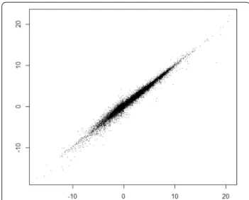
Prediction results are illustrated graphically in Fig. 2, showing good correlation over the whole range of logD values.
After finding optimal settings for the logD model, we developed CCP models with absolute difference, normal-ized, and log-normalized (with β=0 and β =1) noncon-formity measures. We elected to elaborate these models at three epsilon levels starting from 0.001. CPSign error models are necessarily created with the same settings as the endpoint model. However, intuitively it seems that
the task of the error model of explaining mispredictions of logD model is quite difficult, taking into account that
RMSEP=0.41 is already comparable to errors in
experi-mental determinations of logD. Accordingly, the error model can be expected to be less predictive and more prone to overfit than the logD model.
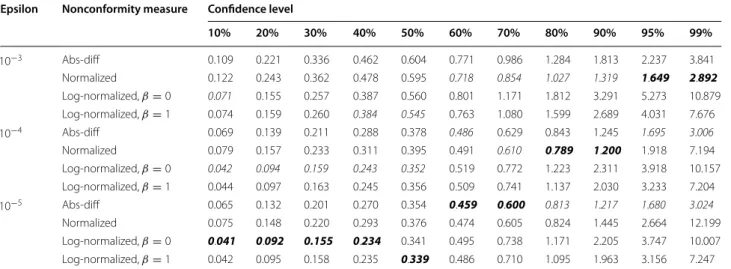
The efficiency of the twelve developed CCP models are presented in Table 2. By comparing models based on absolute difference and the normalized nonconform-ity measure, it is apparent that the later ones are superior at certain ranges of confidence levels—from 50 to 99% when epsilon is 0.001, and from 70 to 90% when epsilon is 10−4. However, the normalized model does not outper-form the absolute difference model when epsilon is 10−5 . This finding confirms the assumption that error models may become overfitted if epsilon is very nonrestrictive.
Another result revealed by Table 2 is the very wide prediction intervals for normalized and log-normalized models at confidence level 99%, indicating that error model based approaches are not of practical use if one wants to achieve such a high confidence level. A some-what surprising finding is that for low confidence lev-els (up to 50%) log-normalized nonconformity measure based models outperform all other models, being how-ever less efficient at higher confidence levels. For exam-ple, if one could be satisfied with 20% confidence, then the median predictions interval width would be below 0.1 log units. Predictions at such a low confidence, however, does not seem to be of any practical use.
The overall-best model at any confidence level is in Table 2 indicated by bolditalics. In most practical CP studies, the desired confidence level is in the range of 80–90% [26, 27, 30–32]. Accordingly, for the prediction service we have selected a model that is most efficient for this range, and in fact, also shows very good efficiency at any other confidence level under 99%.
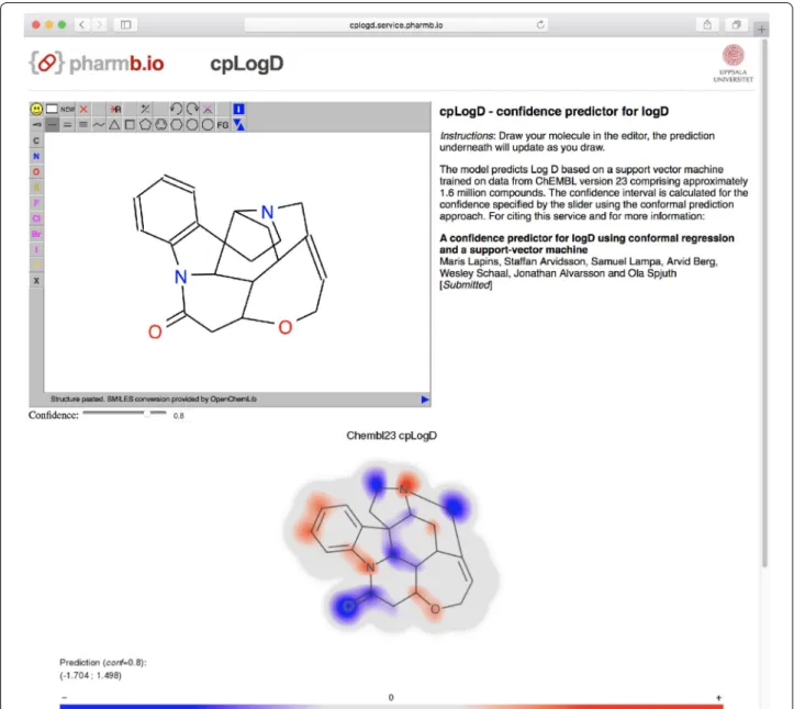
Service for logD prediction
The logD prediction model with normalized noncon-formity measure is available as a REST service using Swagger UI at: https://cplogd.service.pharmb.io/. Swag-ger [33] is a framework for making RESTful web based APIs available. It provides a standard for documentation, code generation as well as the Swagger UI, which is a web based interface where the endpoints of the API can be tested. The logD prediction model is made available with two endpoints:
• /prediction provides a prediction for a given SMILES at a user selected confidence level.
• /predictionImage provides images showing molecule gradient for the prediction.
Table 1 Predictive ability of models, expressed as squared correlation coefficient (Q2) between acd_logd val-ues in ChEMBL database and predicted logD valval-ues for 100,000 test set compounds
Bolditalic values indicate models with the highest predictive ability
Epsilon Cost
0.001 0.01 0.1 1 10
10−1 0.509 0.509 0.510
10−2 0.820 0.821 0.821 0.821
10−3 0.918 0.943 0.949 0.952 0.952
10−4 0.923 0.958 0.970 0.973 0.973
10−5 0.958 0.971 0.973 0.972
Using the swagger service and the free molecule editor JSME [34], we also created a web-based user interface where a prediction image is rendered continuously as a molecule is edited (http://predict-cplogd.os.pharmb.io/ [35]). The user interface also supports selecting a confi-dence level using a slider which will render the prediction interval. Pulling the slider thus gives immediate response on the confidence effect on the prediction interval.
Application of the logD prediction
We will here exemplify prediction results using two ref-erence datasets of experimentally determined logD data.
The 29 compounds selected by Low et al. [36] represent those typically encountered in drug discovery programs, with MW up to 530 and polar surface area up to 114 Å2 . A set of 72 compounds collected by Alelynas et al. [37] shows a broader chemical diversity and range of logD values. In both studies, the literature data is used to vali-date results of newly-developed methods of logD meas-urement and the correlation is reported as R2 of 0.982 and 0.997, respectively, which confirms accuracy of the data. Notably, in ten cases, there is a disagreement of more than one log unit between values reported in [37] and ACD/LogD calculation results, which indicates that affording accurate logD predictions and narrow predic-tion intervals for this dataset is a challenging task.
The prediction results at 80% confidence level are presented graphically in Fig. 3. The prediction is con-sidered correct if the interval includes the true value (i.e., crosses the red-colored identity line). Note the variation in widths of prediction intervals, which for most compounds ranges 0.1–0.8 log units. Among the depicted set of compounds, the two widest intervals are given to strychnine (logD=0.93; prediction midpoint −0.10 and interval from −1.70 to 1.49) and furosemide (logD= −1.02; prediction midpoint −0.46 and interval from −1.44 to 0.51). In both cases, the predictions are
correct. If predictions were performed by absolute differ-ence nonconformity measure, the size of interval for any compound would be 0.843 log units (see Table 2). In this case, prediction intervals for the two “hard to predict” Table 2 Median prediction interval width at confidence levels from 10 to 99%
Shown are MPI at confidence levels (validity) from 10 to 99%. Note that a smaller median prediction interval indicates higher efficiency of a nonconformity measure. Shown are results for models with cost=1 and epsilon values 10−3, 10−4 and 10−5. Italicized are results for the best model at each epsilon value and confidence level.
Marked by bolditalics are results for overall best models at each confidence level
Epsilon Nonconformity measure Confidence level
10% 20% 30% 40% 50% 60% 70% 80% 90% 95% 99%
10−3 Abs-diff 0.109 0.221 0.336 0.462 0.604 0.771 0.986 1.284 1.813 2.237 3.841
Normalized 0.122 0.243 0.362 0.478 0.595 0.718 0.854 1.027 1.319 1.649 2.892 Log-normalized, β=0 0.071 0.155 0.257 0.387 0.560 0.801 1.171 1.812 3.291 5.273 10.879
Log-normalized, β=1 0.074 0.159 0.260 0.384 0.545 0.763 1.080 1.599 2.689 4.031 7.676 10−4 Abs-diff 0.069 0.139 0.211 0.288 0.378 0.486 0.629 0.843 1.245 1.695 3.006 Normalized 0.079 0.157 0.233 0.311 0.395 0.491 0.610 0.789 1.200 1.918 7.194 Log-normalized, β=0 0.042 0.094 0.159 0.243 0.352 0.519 0.772 1.223 2.311 3.918 10.157
Log-normalized, β=1 0.044 0.097 0.163 0.245 0.356 0.509 0.741 1.137 2.030 3.233 7.204 10−5 Abs-diff 0.065 0.132 0.201 0.270 0.354 0.459 0.600 0.813 1.217 1.680 3.024 Normalized 0.075 0.148 0.220 0.293 0.376 0.474 0.605 0.824 1.445 2.664 12.199 Log-normalized, β=0 0.041 0.092 0.155 0.234 0.341 0.495 0.738 1.171 2.205 3.747 10.007
Log-normalized, β=1 0.042 0.095 0.158 0.235 0.339 0.486 0.710 1.095 1.963 3.156 7.247
compounds, strychnine and furosemide, would not include the true value.
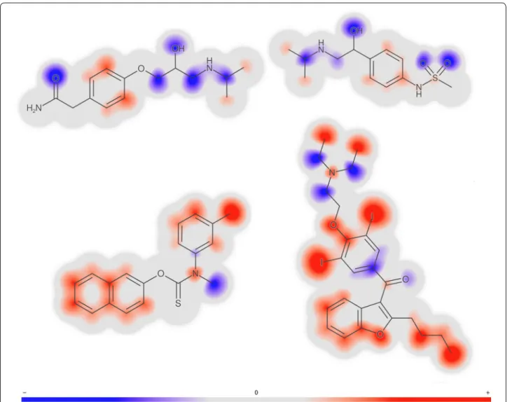
Molecule gradients for the prediction are illustrated in Fig. 4. The red-colored parts of the molecule contribute towards a prediction of higher logD and the blue parts contribute towards a prediction of lower logD. Note that the two hydrophilic compounds, atenolol and sotalol, are predominantly colored blue, except the phenyl rings that are colored light red and thus are predicted to increase lipophilicity. Note also that the propan-2-ylamino groups present in both compounds have similar but not exactly the same coloring. This is because each atoms is assessed in its environment of up to a three-bond distance (i.e., from all signatures of height one to three that include the given atom). In contrast to hydrophilic compounds at the top of the figure, the two highly lipophilic compounds at
the bottom are predominantly colored red, except for the amine and ketone groups that are expected to decrease logD.
Figure 5 illustrates a molecular gradient for a com-pound with a wide prediction interval, rendered in the user interface of prediction service at http://predict-cplogd.os.pharmb.io/. For this polycyclic alkaloid, the model has created quite a complex molecule gradient. In the upper panel of the interface a user can interactively modify molecule to inspect quantitative contribution of any modified atom(s) to the prediction of logD and to the width of the prediction interval.
Dataset publication as RDF
in W3C RDF format [38]. It is available for download as data dumps in the Turtle RDF serialization format [39] and the indexed, binary RDF HDT format [40, 41] at https://doi.org/10.5281/zenodo.1091111 [42]. A URI resolver service is available at https://rdf.pharmb.io [43]. The URI resolver resolves the URIs of the new triples cre-ated for this dataset. It does so by providing all the tri-ples linked to the resolved URI in N-Tritri-ples format [44] when accessing the URI via HTTP GET (the same as vis-iting the URL in a web browser). Newly created URIs for descriptors and compounds were minted off of the base
URI resolver software called urisolve was developed. The urisolve software resolves URI:s in a dataset based on an RDF HDT file or a SPARQL endpoint [47]. This software is available as open source at https://github.com/pharm-bio/urisolve [48]. The urisolve software makes use of the RDF library for Go by Petter Goksøyr Åsen [49] for RDF serialization and the C++ HDT tools [50] for accessing the RDF HDT file.
Conclusions
We have developed a confidence predictor for chemical compound lipophlicity (logD) using molecular signature descriptors and a support-vector machine. Unlike con-ventional regression, confidence predictor produces pre-diction intervals that satisfy a required confidence level. With normalized nonconformity measure, individual intervals are calculated for each compound. Model vali-dation shows that the median prediction intervals (±0.39 log units at 80% confidence and ±0.60 log units at 90% confidence) are tight enough to be useful in discovery.
The model is available as an online service via an OpenAPI interface and a web page with a molecular editor. Molecular signature descriptors allow interactive modifi-cation of molecules and visual interpretation of prediction results by highlighting chemical substructures contribut-ing to the increase/decrease of the predicted logD.
We have also published predictive values at 90% confi-dence level for 91 million compounds of PubChem database in RDF format for download and as an URI resolver service. Authors’ contributions
OS, JA, SA and WS conceived the study. ML and SA designed and imple-mented the modeling components and performed data analysis. JA, SA and AB implemented the prediction service. SL, AB and WS implemented dataset publication in RDF format and URI resolver service. All authors read and approved the final manuscript.
Acknowledgements
This study was supported by OpenRiskNet (Grant Agreement 731075), a project funded by the European Commission under the Horizon 2020 Programme.
Competing interests
OS hold shares in Genetta Soft AB, a Swedish incorporated company.
Ethics approval and consent to participate
Not applicable.
Publisher’s Note
Springer Nature remains neutral with regard to jurisdictional claims in pub-lished maps and institutional affiliations.
Received: 21 December 2017 Accepted: 25 March 2018
References
1. Kerns EH, Di L (2003) Pharmaceutical profiling in drug discovery. Drug Discov Today 8(7):316–323
2. Waring MJ (2010) Lipophilicity in drug discovery. Expert Opin Drug Discov 5(3):235–248
3. Hann MM, Keseru GM (2012) Finding the sweet spot: the role of nature and nurture in medicinal chemistry. Nat Rev Drug Discov 11(5):355–365 4. Waring MJ (2009) Defining optimum lipophilicity and molecular weight ranges for drug candidates—molecular weight dependent lower logD limits based on permeability. Bioorg Med Chem Lett 19(10):2844–2851 5. Johnson TW, Dress KR, Edwards M (2009) Using the Golden Triangle
to optimize clearance and oral absorption. Bioorg Med Chem Lett 19(19):5560–5564
6. Leeson PD, Springthorpe B (2007) The influence of drug-like concepts on decision-making in medicinal chemistry. Nat Rev Drug Discov 6(11):881–890
7. Hughes JD, Blagg J, Price DA, Bailey S, Decrescenzo GA, Devraj RV, Ellsworth E, Fobian YM, Gibbs ME, Gilles RW, Greene N, Huang E, Krieger-Burke T, Loesel J, Wager T, Whiteley L, Zhang Y (2008) Physiochemical drug properties associated with in vivo toxicological outcomes. Bioorg Med Chem Lett 18(17):4872–4875
8. Waring MJ, Johnstone C (2007) A quantitative assessment of hERG liabil-ity as a function of lipophilicliabil-ity. Bioorg Med Chem Lett 17(6):1759–1764 9. Wager TT, Hou X, Verhoest PR, Villalobos A (2010) Moving beyond rules: the development of a central nervous system multiparameter optimiza-tion (CNS MPO) approach to enable alignment of druglike properties. ACS Chem Neurosci 1(6):435–449
10. Mannhold R, Poda GI, Ostermann C, Tetko IV (2009) Calculation of molecular lipophilicity: state-of-the-art and comparison of log P methods on more than 96,000 compounds. J Pharm Sci 98(3):861–893
11. ACD/Labs.com. www.acdlabs.com. Accessed 01 Nov 2017 12. Gaulton A, Hersey A, Nowotka M, Bento AP, Chambers J, Mendez D,
Mutowo P, Atkinson F, Bellis LJ, Cibrian-Uhalte E, Davies M, Dedman N, Karlsson A, Magarinos MP, Overington JP, Papadatos G, Smit I, Leach AR (2017) The ChEMBL database in 2017. Nucleic Acids Res 45(D1):945–954 13. Jeliazkova N, Jeliazkov V (2011) AMBIT RESTful web services: an
imple-mentation of the OpenTox application programming interface. J Chemin-form 3:18
14. Jeliazkova N, Kochev N (2011) AMBIT-SMARTS: efficient searching of chemical structures and fragments. Mol Inform 30(8):707–720 15. Willighagen EL, Mayfield JW, Alvarsson J, Berg A, Carlsson L, Jeliazkova N,
Kuhn S, Pluskal T, Rojas-Cherto M, Spjuth O, Torrance G, Evelo CT, Guha R, Steinbeck C (2017) The chemistry development kit (CDK) v2.0: atom typing, depiction, molecular formulas, and substructure searching. J Cheminform 9(1):33
16. Kim S, Thiessen PA, Bolton EE, Chen J, Fu G, Gindulyte A, Han L, He J, He S, Shoemaker BA, Wang J, Yu B, Zhang J, Bryant SH (2016) PubChem sub-stance and compound databases. Nucleic Acids Res 44(D1):1202–1213 17. Faulon JL, Visco DP, Pophale RS (2003) The signature molecular descriptor.
1. Using extended valence sequences in QSAR and QSPR studies. J Chem Inf Comput Sci 43(3):707–720
18. CPSign. http://cpsign-docs.genettasoft.com. Accessed 04 Dec 2017 19. Spjuth O, Eklund M, Ahlberg Helgee E, Boyer S, Carlsson L (2011)
Integrated decision support for assessing chemical liabilities. J Chem Inf Model 51(8):1840–7. https://doi.org/10.1021/ci200242c
20. Alvarsson J, Eklund M, Andersson C, Carlsson L, Spjuth O, Wikberg JE (2014) Benchmarking study of parameter variation when using signature fingerprints together with support vector machines. J Chem Inf Model 54(11):3211–3217
21. Vapnik V (1998) Statistical learning theory. Wiley, New York
22. Alvarsson J, Lampa S, Schaal W, Andersson C, Wikberg JE, Spjuth O (2016) Large-scale ligand-based predictive modelling using support vector machines. J Cheminform 8:39
23. Fan R-E, Chang K-W, Hsieh C-J, Wang X-R, Lin C-J (2008) LIBLINEAR: a library for large linear classification. J Mach Learn Res 9:1871–1874 24. Vovk V, Gammerman A, Shafer G (2005) Algorithmic learning in a random
world. Springer, New York
25. Papadopoulos H, Haralambous H (2011) Reliable prediction intervals with regression neural networks. Neural Netw 24(8):842–851
27. Cortes-Ciriano I, Bender A, Malliavin T (2015) Prediction of PARP inhibition with proteochemometric modelling and conformal prediction. Mol Inform 34(6–7):357–366
28. Vovk V (2015) Cross-conformal predictors. Ann Math Artif Intell 74(1–2):9–28
29. Carlsson L, Helgee EA, Boyer S (2009) Interpretation of nonlinear QSAR models applied to ames mutagenicity data. J Chem Inf Model 49(11):2551–2558
30. Cortes-Ciriano I, van Westen GJ, Bouvier G, Nilges M, Overington JP, Bender A, Malliavin TE (2016) Improved large-scale prediction of growth inhibition patterns using the NCI60 cancer cell line panel. Bioinformatics 32(1):85–95
31. Norinder U, Rybacka A, Andersson PL (2016) Conformal prediction to define applicability domain: a case study on predicting ER and AR bind-ing. SAR QSAR Environ Res 27(4):303–316
32. Lindh M, Karlen A, Norinder U (2017) Predicting the rate of skin penetra-tion using an aggregated conformal predicpenetra-tion framework. Mol Pharm 14(5):1571–1576
33. https://swagger.io. Accessed 04 Dec 2017
34. Bienfait B, Ertl P (2013) JSME: a free molecule editor in javascript. J Chem-inform 5(1):24. https://doi.org/10.1186/1758-2946-5-24
35. http://predict-cplogd.os.pharmb.io/. Accessed 04 Dec 2017 36. Low YW, Blasco F, Vachaspati P (2016) Optimised method to estimate
octanol water distribution coefficient (logD) in a high throughput format. Eur J Pharm Sci 92:110–116
37. Alelyunas YW, Pelosi-Kilby L, Turcotte P, Kary MB, Spreen RC (2010) A high throughput dried dmso logd lipophilicity measurement based on 96-well shake-flask and atmospheric pressure photoionization mass spectrom-etry detection. J Chromatogr A 1217:1950–1955
38. https://www.w3.org/TR/rdf11-concepts/. Accessed 04 Dec 2017 39. https://www.w3.org/TR/turtle/. Accessed 04 Dec 2017
40. Fernández JD, Martínez-Prieto MA, Gutiérrez C, Polleres A, Arias M (2013) Binary RDF representation for publication and exchange (HDT). Web Semant 19:22–41
41. Martínez-Prieto MA, Gallego MA, Fernández JD (2012) Exchange and consumption of huge RDF data. In: Lecture notes in computer science (including Subser Lect Notes Artif Intell Lect Notes Bioinformatics) 7295 LNCS. pp 437–452
42. Lapins M, Arvidsson S, Lampa S, Berg A, Schaal W, Alvarsson J, Spjuth O (2017) RDF Dataset: A confidence predictor for logD using confor-mal regression and a support-vector machine. Zenodo. https://doi. org/10.5281/zenodo.1091111
43. https://rdf.pharmb.io/cplogd. Accessed 04 Dec 2017 44. https://www.w3.org/TR/n-triples/. Accessed 04 Dec 2017 45. Dumontier M, Baker CJ, Baran J, Callahan A, Chepelev L, Cruz-Toledo
J, Klassen D (2014) The semanticscience integrated ontology (SIO) for biomedical research and knowledge discovery. J Biomed Semant 5:14 46. Fu G, Batchelor C, Dumontier M, Hastings J, Willighagen E, Bolton E (2015)
PubChemRDF: towards the semantic annotation of PubChem compound and substance databases. J Cheminform 7:34