4698.pdf

LONGITUDINAL MULTI-TRAIT-STATE-METHOD MODEL USING ORDINAL DATA

Richard Shane Hutton

A thesis submitted to the faculty of the University of North Carolina at Chapel Hill in partial fulfillment of the requirements for the degree of Master of Arts in the Department of Psychology (Quantitative).

Chapel Hill 2012

Approved by

Sy-Miin Chow, Ph.D. Robert MacCallum, Ph.D.

c

2012

Richard Shane Hutton

ABSTRACT

RICHARD SHANE HUTTON: Longitudinal Multi-Trait-State-Method Model using Ordinal Data

(Under the direction of Sy-Miin Chow)

Multi-trait multi-method (MTMM) models were designed as a way to assess

con-vergent and discriminant validity using multiple traits measured by multiple

meth-ods. In recent years, longitudinal extensions of multi-trait multi-method models have

been proposed in the structural equation modeling framework to evaluate whether

and how the trait as well as method factors change over time. This thesis is intended

to propose a longitudinal second-order multi-trait-state-method (M-TSM) model that

combines a measurement model for ordinal data, a vector autoregressive moving

av-erage (VARMA) model at the latent level to examine changes in the state as well as

method factors over time, and a second-order factor analytic model to capture shared

trait variances among the state affect factors. A set of affect items from the Affective

Dynamics and Individual Differences (Emotions and Dynamic Systems Laboratory,

2010) study was used to illustrate the proposed longitudinal M-TSM model. This

study features affect items asked in both a lab and a diary setting. Results of the

fi-nal model showed that the method factors, lab and diary, had perfect stability across

time. Furthermore, factor loadings within the lab factor showed a systemic pattern of

positive and negative loadings illustrating the complexity of individuals’ affective

re-sponses to stimuli in the lab setting. Contrary to conventional theories on emotions,

the covariances between positive and negative affect factors at the state level were not

significantly different from zero; however, evaluation of higher-order shared

between the two at the “trait” level. Comparisons of the auto- and cross-regression

regression parameters associated with the state affect factors indicated some key

dif-ferences in how people regulated negative emotions in a lab versus in a diary setting.

TABLE OF CONTENTS

List of Tables . . . vii

List of Figures . . . .viii

CHAPTER

1.1 Multi-Trait Multi-Method (MTMM) . . . 2

1.1.1 Multi-Trait Multi-Method Matrix . . . 3

1.2 Structural Equation Modeling (SEM) . . . 6

1.2.1 Multi-Trait Multi-Method SEM Models . . . 7

1.2.2 Ordinal Measurement Model . . . 10

1.3 Item Response Theory . . . 12

1.4 Longitudinal Models . . . 14

1.4.1 Longitudinal Multi-Trait Multi-Method . . . 14

1.4.2 Time Series Analysis . . . 15

1.4.3 Invariance . . . 17

1.5 Objectives for Thesis . . . 19

2 Methods . . . 20

2.1 Illustrative Example . . . 20

2.1.1 Participants and Measures . . . 20

2.1.2 Procedures . . . 21

2.2 Model Descriptions . . . 22

2.2.2 Item Exploratory Analysis . . . 22

2.2.3 Longitudinal M-TSM Model for the PANAS Data . . . 23

3 Results . . . 31

3.1 Results for Item Analysis . . . 31

3.1.1 IRT Analyses . . . 31

3.1.2 Establishing Longitudinal Invariance . . . 32

3.2 Most Parsimonious Model . . . 33

4 Discussion . . . 42

LIST OF TABLES

2.1 Models Used to Examine Longitudinal Invariance in the PANAS Items. . . 28

3.1 Final List of PANAS Items Retained. . . 32

3.2 Models Used to Examine Perfect Stability in the Method Factors . . . 35

3.3 Factor Loadings for the Most Parsimonious Model . . . 36

3.4 Random Shock Variance Estimates for the Most Parsimonious Model . . . 39

LIST OF FIGURES

1.1 Synthetic multitrait-multimethod matrix taken from Campbell and Fiske

(1959), pg. 82. . . 5

1.2 Example of a SEM-MTMM model. . . 8

1.3 Example of a correlated trait-correlated method model. . . 9

1.4 Example of a correlated trait-correlated uniqueness model. . . 10

1.5 Example of a correlated trait-correlated method minus one model. . . 11

2.1 Example of (a) a“more desirable” item and (b) a “less desirable” item. . . . 23

2.2 Path diagram of a longitudinal M-TSM model with VAR(1) relationships at the factor level. . . 27

3.1 Trace lines for “irritable”. . . 34

CHAPTER 1

Introduction

Multi-trait multi-method (MTMM) models have long been used by behavioral

and social scientists to study different traits assessed by different methods (e.g.,

Winne & Marx, 1977; Waksman, 1978; Andrews, 1984; Bagozzi & Yi, 1991; Luzzo,

1993). Longitudinal MTMM models provide one possible way for researchers to

study how traits assessed by various methods vary over time. Such models not only

allow researchers to examine whether or not traits are changing over time, but also

provide a proxy for studying the stability of the assessment methods over time.

Sta-bility is a key feature that distinguishes trait processes from state processes. Trait

processes refer to stable constructs that remain relatively constant over time;

how-ever,stateprocesses refer to volatile constructs that change on a moment-to-moment

basis (Nesselroade & Bartsch, 1977).

With ecological momentary assessment designs such as experience sampling and

daily diary designs becoming increasingly popular (Iida, Shrout, Laurenceau, &

Bol-ger, in press), it is important to develop a longitudinal model that is suited for

rep-resenting the kind of less structured, “state-like” changes often seen in such data.

While longitudinal variations of MTMM models have been proposed by other

re-searchers, the change processes assumed in such models are typically structured

growth processes that are relatively smooth Grimm, Pianta, & Konold, 2009; Cole,

Ecological momentary assessment data, in contrast, are often characterized by less

systematic ebbs and flows driven by external shocks or events.

The purpose of this thesis is to propose a longitudinal second-order MTMM

model that combines a vector autoregressive moving average (VARMA) model at the

latent level and a measurement model for ordinal data to represent relatively volatile

change processes over time. The VARMA model included in the proposed

longitudi-nal MTMM model is especially suited for representing fluctuations in state processes.

In this way, the proposed model is a multi-“state” multi-method longitudinal model

at the first-order level and will be referred to as a multi-trait-state-method model

(M-TSM). Another major issue the proposed model serves to address is how MTMM

models may be adapted for use with ordinal data. Likert-type items are relatively

common in social and behavioral sciences. Proper modeling techniques are needed

to handle the ordinal nature of this type of data.

The introduction is organized as follows. I first introduce the MTMM design

and define construct validity followed by a discussion of the original MTMM matrix.

Next, structural equation modeling (SEM)—the modeling framework in which the

proposed longitudinal M-TSM model is structured—as well as various SEM-MTMM

models are introduced. In addition, a discussion of the ordinal measurement model

is given. I then present an introduction to item response theory, particularly the

graded response model, which is used to evaluate the psychometric properties of

a set of items to be used for model fitting purposes. Finally, an overview of the

VARMA model is given followed by a discussion of the importance of longitudinal

measurement invariance.

1.1 Multi-Trait Multi-Method (MTMM)

A MTMM design consists of the measurement of at least two traits using at least

two assessment methods (Campbell & Fiske, 1959). Not only are multiple methods of

need to understand whether or not these methods measure what they are intended to

measure. As such, violations of construct validity constitute a source of confound in

scientific studies. That is, researchers have the task of determining if their measures

are adequately representing the construct of interest.

In discussing MTMM, it is useful to first review the concepts of convergent,

dis-criminant and construct validity. Construct validity answers the question: are we

measuring what we intend to measure? That is, is there an association between the

measures and the theoretical construct they are purported to measure? Furthermore,

construct validity can be decomposed into two subparts: convergent and

discrimi-nant validity. Convergent validity helps determine whether or not the measures that

are supposed to be related actually are. Conversely, discriminant validity helps

de-termine whether or not the measures that are not supposed to be related actually are

not.

1.1.1 Multi-Trait Multi-Method Matrix

For decades, the MTMM Matrix has been used to examine convergent,

discrim-inant and construct validity. The MTMM Matrix is a correlation matrix that

rep-resents the intercorrelations between trait and method factors. Figure 1.1 shows

a classic MTMM matrix taken from Campbell et Fiske (1959). This synthetic

ma-trix is a correlation mama-trix composed of the correlations among three different traits

measured using three different methods. While all of the off-diagonal elements

rep-resent correlations, each of the diagonal elements of the MTMM matrix consists of

the reliability estimate of one particular measure. The solid triangles represent the

monomethod triangles and the dashed triangles represent the

heterotrait-heteromethod triangles. The heterotrait-monomethod triangles represent correlations

that share the same measurement method. Conversely, the heterotrait-heteromethod

triangles represent correlations that do not share the same measurement method.

di-agonals. These diagonals represent the correlations between measures of the same

trait but assessed using different methods.

The validity diagonal contains information about convergent validity. That is,

high correlations between measures of the same trait would be expected even if

dif-ferent methods are being used. For example, in Figure 1.1 the correlations along the

validity diagonal are relatively high in comparison with the neighboring correlations.

The neighboring correlations in the heterotrait-heteromethod triangles represent the

correlations between different traits and methods. This provides information about

discriminant validity; namely, these measures should have low correlations because

they are not related. Finally, the heterotrait-heteromethod triangles allow for the

examination of a method effect. That is, if relatively high correlations exist within

these triangles, then the methods are having a strong influence since none of these

correlations share the same trait.

The MTMM matrix has several limitations; one major limitation lies in the

diffi-culties for researchers to quantify and infer the existence of construct validity simply

by eyeballing the correlations. That is, there is no set standard to help gauge whether

the different kinds of validity are attained. It is also impossible to separate method

and error variances, which may lead to spurious correlations and wrong conclusions

(Schmitt & Stults, 1986). Finally, the MTMM matrix requires the measures to be

con-ditionally independent once the shared variances attributable to common method

and common trait have been accounted for (Campbell & Fiske, 1959); whereas, in

reality correlations might exist between method factors and trait factors. Given these

limitations of the MTMM matrix, many researchers have turned to a statistical

tech-nique called structural equation modeling (SEM) as an alternative method for

1.2 Structural Equation Modeling (SEM)

SEM is a set of statistical techniques that allows for the evaluation of relationships

among variables, specifically, the relationships between observed variables (usually

called manifest variables) and unobserved latent variables. SEM is also known as

covariance structure modeling because some of the earliest structural equation

mod-els focus explicitly on representing the covariance structures among measured and

latent variables (J ¨oreskog, 1973, 1974a). In order to describe these relationships, two

models are defined: 1) the measurement model and 2) the structural model. The

measurement model relates the manifest variables to the latent variables; whereas,

the structural model relates the latent variables to each other.

The measurement model consists of two equations. One equation links manifest

variables and exogenous latent variables and a second equation links manifest

vari-ables and endogenous latent varivari-ables. The first measurement equation is defined

as

xit =υx+Λxξ_i+δi (1.1)

where xit is a q × 1 vector of manifest variables for person i, υ is a q × 1 vector

of intercepts, Λx is a q × n factor loading matrix, ξ_i is an n × 1 vector of latent

exogenous variables for person i, and δi is aq ×1 vector of measurement errors. It

is assumed thatδi is normally distributed, ξ_i and δi are uncorrelated and both have

expected values of zeroes.

The second measurement equation is defined as

y_i =υy+Λyηi+εi (1.2)

where y_i is a p × 1 vector of manifest variables for person i, υy is a p × 1 vector

endogenous variables for person i, and εi is a p × 1 vector of measurement errors.

Once again, it is assumed that ε_i is multivariate normally distributed with a vector

of zeroes as expected values and covariance matrix, Ψ. In addition, η_i and ε_i are

assumed to be uncorrelated.

Finally, the structural model is defined as

η_i =α+Bη_i+Γξ_i+ζ_i (1.3)

where α is a m × 1 vector of intercepts, B is an m × m matrix linking the latent

endogenous variables, Γ is an m × n matrix linking the latent exogenous variables

to the latent endogenous variables and ζ_i is a m ×1 vector of residual errors which

is assumed to be multivariate normally distributed with zero means and covariance

matrix Ψ.

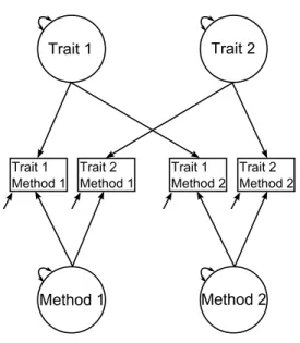
1.2.1 Multi-Trait Multi-Method SEM Models

Thus far, I have introduced the MTMM matrix developed by Campbell and Fiske

(1959) and provided a brief introduction to the SEM framework. Next, I will review

how the MTMM design and how pertinent validity-related questions can be

formu-lated as part of a structural equation model. Central to the SEM-MTMM framework

is a set of latent variables representing traits and a second set of latent variables

representing methods. Each manifest variable loads onto one trait and one method.

Figure 1.2 shows an example of a basic SEM-MTMM. Note that this model consists

of only endogenous latent variables; that is, there is no exogenous component. In

addition, the trait and method factors are uncorrelated with one another. Over the

years, several different SEM-MTMM models have been formulated. I will provide a

quick review of the primary models.

The Correlated Trait-Correlated Method Model. The correlated trait-correlated

Trait 1 Method 1

Trait 2 Method 1

Trait 1 Method 2

Trait 2 Method 2

Method 1 Method 2

Trait 1 Trait 2

Figure 1.2: Example of a SEM-MTMM model.

resembles the original MTMM matrix validity defined by Campbell and Fiske (1959)

due to its formulation and interpretation; an example is shown in Figure 1.3. This

model has a latent variable for each trait and each method. Furthermore, correlations

exist between the trait factors and sometimes also the method factors; however, there

is no correlation between method and trait factors. One major benefit of this model

is the ease of interpretation. Large trait factor loadings represent convergent validity

and small correlations between trait factors represent discriminant validity. Thus,

validity is defined in much the same ways as how Campbell and Fiske (1959)

origi-nally defined validity. The major disadvantage of these models lies in problems with

identification and convergence (Marsh, 1989; Marsh & Bailey, 1991); issues include

(1) underidentified models, (2) negative variances and (3) correlations outside of the

proper range. While other models are not immune from these issues, they are most

prevalent in the correlated trait-correlated method model.

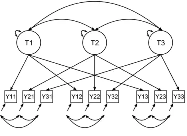
The Correlated Trait-Correlated Uniqueness Model. The correlated trait-correlated

trait-M1 T1

Y11 Y21 Y31

M2 T2

Y12 Y22 Y32

M3 T3

Y13 Y23 Y33

Figure 1.3: Example of a correlated trait-correlated method model.

correlated method model but method factors are not specified explicitly (see Figure

1.4). Instead, to account for the method effects, error terms are allowed to be

corre-lated within methods, with no correlations allowed between the errors of manifest

variables measured using different methods. Not allowing for correlations between

the errors of different methods is equivalent to assuming that the methods factors

in Figure 1.3 are independent, which may be overly restrictive in some applications.

Furthermore, another limitation is that the error terms represent both measurement

errors and the residual effects that are idiosyncractic to each method; it is not possible

to decompose the two. This model does have the advantage of fewer identification

problems than the correlated trait-correlated method model proposed by Widaman

(1985).

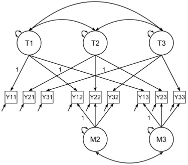
The Correlated Trait-Correlated Method Minus One Model. The correlated

trait-T1

Y11 Y21 Y31

T2

Y12 Y22 Y32

T3

Y13 Y23 Y33

Figure 1.4: Example of a correlated trait-correlated uniqueness model.

correlated method model (J ¨oreskog, 1974b; Widaman, 1985), except that one method

serves as a reference method (see Figure 1.5). This latter model is nested within the

correlated-trait correlated-method model, with special constraints included in the

factor loading matrix. That is, the loadings of the manifest measures on one of the

method factors - namely, the reference method - are fixed at zeroes. This implies

that there are no shared sources of variance among the manifest variables measured

using the reference method after the shared variance due to trait has been extracted.

In addition, the loadings of the trait factors on manifest variables measured using

the reference method are set to one as added identification constraints. The

ma-jor advantage of this model is that by imposing more identification constraints than

the standard correlated-trait correlated-method model, convergence issues are

re-duced; however, it can be difficult to determine which method to use as the reference

method.

1.2.2 Ordinal Measurement Model

The measurement model shown in Equations 1.1 & 1.2 assumes that continuous

indica-T1

Y11 Y21 Y31

M2 T2

Y12 Y22 Y32

M3 T3

Y13 Y23 Y33

1 1

1 1 1

Figure 1.5: Example of a correlated trait-correlated method minus one model.

tors requires a different measurement model to be specified. One common way of

incorporating ordinal manifest variables is to use an ordered probit link. The basic

assumption made is that responses to the ordinal observed measured variablesyare

influenced by an unobserved, continuous measured variable y∗. Therefore, only

re-sponse categories are observed. That is, for ordered rere-sponse categoriesk =1, 2, ...,m,

thresholds are defined as

yi,j=k ifτj,k−1<y∗ ≤τj,k (1.4)

where τj,k are threshold parameters for the jth items. The thresholds represent

cut-points on the continuous latent variable y∗ that determine whether respondents

en-dorse a particular category k on the jth observed item y. When a probit link is

specified, the cumulative distribution function (CDF) ofy∗ is assumed to be normal.

section. When estimating ordered categorical indicators in SEM, error terms for the

indicators are not being estimated; instead, the threshold parameters, τj,k, are

esti-mated. Furthermore, treating the ordered categorical items as continuous would not

be appropriate and could lead to spurious results (DiStefano, 2002). Various

estima-tion methods for handling categorical data in SEM have been summarized by Wirth

and Edwards (2007).

1.3 Item Response Theory

Item Response Theory (IRT) is a set of statistical models that relates the

proba-bility of an individual’s response on an item as a function of item parameters and

an underlying latent trait (Lord, 1980). In contrast to the SEM framework presented

above, commonly used IRT models assume a logit link for y; that is, IRT uses a

lo-gistic distribution function instead of a normal distribution function (probit) as the

CDF for the continuous latent variable,y∗. One important advantage of using IRT is

that the various estimation procedures and associated software packages have been

developed specifically to handle large-scale categorical data sets. Thus, the

assess-ment of psychometric properties of categorical items, including ordinal items, can be

performed in a computationally efficient manner.

In the IRT framework, two item-related parameters are typically of primary

inter-est: discrimination and difficulty parameters. Discrimination represents how related

an item is to the latent trait; whereas, difficulty represents the trait level needed so

that there is a 0.5 probability of endorsing a particular item (in the case of binary

items) or response category (in the case of ordinal items). An item that is highly

discriminating provides more information about the latent construct than a item that

is less discriminating. A one-parameter IRT model estimates the difficulty

param-eter for each item; whereas, a two-paramparam-eter model estimates both difficulty and

discrimination.

and the type of data used. For ordinal data, one commonly used model is the graded

response model (Samejima, 1969). The graded response model is a two-parameter

model and it postulates that the probability for individual i to endorse the kth or

other higher response categories (k=1, 2, . . . ,m), is defined as

P(yij ≥k|θi,aj,bj,k) = Pj,k(θi) = 1

1+exp[−aj(θi−bj,k)]

(1.5)

where the equation represents the probability of responding in category k or higher

given θ, the individual’s latent trait level. The parameter aj is the discrimination

parameter for item j and bj,k is the kth difficulty parameter for the jth item. In

other words, Equation 1.5 provides a probabilistic representation of responding in a

particular category or higher given a certain level ofθ.

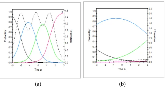
A graphical representation of the differences between the conditional response

probabilities of adjacent response categories are known as trace lines (also called item

characteristic curves). That is, a trace line is the difference between the probabilities

of two adjoining categories, corresponding to P(yij =k|θi,aj,bj,k). Mathematically, a

trace line,Tj, for item j and category k are represented as

Tj = 1

1+exp[−aj(θi−bj,k−1)]

− 1

1+exp[−aj(θi−bj,k)]

=T_j∗(k)−T_j∗(k+1)

(1.6)

Additionally, information curves help to determine how much information an

item gives us to estimate different levels of θ. Information determines at what levels

of θ an item is best at discriminating between individuals. That is, higher

informa-tion allows for more precision in measuring θ. It is important to note that IRT and

the ordinal measurement model in the SEM framework are mathematically

expressed as

aj = (

λj

q

1−λ2_j

)D and bj,k =

τj,k

λj

(1.7)

where λi is the factor loading1 for the jth item, D = 1.7 is the scaling factor, and τj,k

is the threshold for the jth item.

Finally, in order to properly estimate the item parameters, IRT models require a

set of locally independent items (i.e no local dependence). That is, item responses are

independent from each other controlling for trait level. There are multiple statistics

to evaluate local dependence; the χ2 LD statistic (Chen & Thissen, 1997) will be

used. The χ2 LD statistic examines the covaration between observed and expected

frequencies between pairs of items. This covariation should be zero if there is no

local dependence; however, if this covaration differs significantly then there exists

local dependence between a pair of items (i.e. violation of local independence).

1.4 Longitudinal Models

1.4.1 Longitudinal Multi-Trait Multi-Method

The idea of using MTMM longitudinally was first introduced by Werts, J ¨oreskog

and Linn (1972) to study growth. Since then, several longitudinal MTMM models

have been proposed to date (Conley, 1985; Cudeck, 1985; Burns, Walsh, & Gomez,

2003; Marsh & Grayson, 1995; Scherpenzeel & Saris, 2007). This section is intended to

briefly summarize the various longitudinal MTMM models that have been proposed

within the SEM framework.

Grimm et al. (2009) presented a longitudinal version of the correlated

trait-correlated method model wherein changes in the trait factors over time are

repre-sented using second-order latent growth curve models. In addition to using growth

curve models to examine linear changes in the trait factors, they also tested the

variance of the repeated measures over time. The authors noted several convergence

issues with their model especially when the correlations are high among factors.

Furthermore, the authors suggested building the model at each time point prior to

incorporating all repeated measures to evaluate trends or changes over time to aid

estimation difficulties.

Cole et al. (1996) formulated a longitudinal correlated trait-correlated

unique-ness model to study the relationship between social and academic competence and

depression using two waves of data. In line with properties of the cross-sectional

correlated trait-correlated uniqueness model (Kenny, 1976; Marsh, 1989), errors of

the same measures were allowed to be correlated across as well as within waves.

The authors also used correlations to examine stability across waves of data using a

test-retest type of design. Finally, Geiser et al. (2010) presented a longitudinal

ver-sion of the correlated trait-correlated method minus one model in which the latent

difference model (McArdle & Hamagami, 2001b) was used to represent changes in

the trait factors over time.

The longitudinal MTMM models reviewed above are similar in that the

correla-tions between trait factors over time are hypothesized to stem from some forms of

structured growth curve processes2; however, none of the models employ time series

techniques. Furthermore, the proposed model uses three waves of data, which is

more beneficial than two waves of data typically used in the aforementioned models

(Willett, 1989).

1.4.2 Time Series Analysis

Time series analysis is a set of statistical methods for analyzing time series data,

namely, data that are collected over time. Two commonly used univariate time series

models are autoregressive and moving average processes (Chatfield, 2004; Wei, 1990;

2_{The latent difference score models proposed by McArdle and colleagues (2001b) can be regarded}

Hamilton, 1994). Time series models are traditionally used with single-subject time

series data with many repeated measurement occasions. Thus, the subject index is

typically omitted from the corresponding models. Here, these models are used with

multiple-subject longitudinal panel data with many participants and relatively few

time points. I therefore include a subject index in all the equations that follow.

Mathematically, an autoregressive model of lag order r, denoted as AR(r), for a

measured variable,yit, of personi at timet, is defined as

yit = r

∑

u=1

ϕuyi,t−u+εit (1.8)

whereϕu(u=1, . . .,r) are autoregressive parameters andεitis an error term. Browne

and Nesselroade (2005) referred to these “errors” as random shocks because they can

be regarded as shocks whose impact continues to affect later yit. In the case of

the AR process, the lagged effects of such shocks are transmitted through previous

yit. The error term εit has the following assumptions: zero mean, variance σ2, and

uncorrelated for different time values. Furthermore, r is the highest lag order of

the process and the AR processes is considered to be weakly stationary if E[yit] and

Var[yit]are constant (Chatfield, 2004)

In a similar vein, a moving average model of lag orders, denoted as MA(s), for a

measured variable yit, is defined as

yit= s

∑

v=1

δvεi,t−v+εit (1.9)

whereδv are moving average parameters andεitis an error term or random shock. A

moving average process is considered to be invertible if it can be rewritten as a linear

combination of its past values (Chatfield, 2004). Both equations 1.8 and 1.9 can be

combined to yield an auto-regressive moving-average (ARMA) model of order (r, s).

of the univariate AR(r) and MA(s) models shown in Equations 1.8 and 1.9. The

VARMA model can be structured within the SEM framework wherein a series of

autoregressive and moving average components are represented in the structural

equation. For example, combining Equations 1.8 and 1.9 the VARMA(r,s) model is

obtained

y_it=

r

∑

u=1

ϕuy_i,t−u + s

∑

v=1

δvεi,t−v+εit (1.10)

where y_it is now a vector of manifest variables and ε_it is the corresponding vector

of random shocks. Multiple researchers have evaluated variations of univariate and

multivariate time series models in the context of SEM, (e.g., McArdle & Hamagami,

2001a; Bollen & Curran, 2004), but no work has been done combining SEM-MTMM

models with time series analysis. Not only do autoregressive parameters allow for

the examination of the influence of one time point on another, they offer a

straight-forward index for evaluating the stability of a construct of interest over time. In

addition, cross-regression parameters allow researchers to examine the influence of

past constructs on other constructs of interest. More importantly, times series models

are suited for representing less structured change processes typically seen in state

fluctuations, such as those evidenced in emotions data.

1.4.3 Invariance

In the study of longitudinal change processes, it is useful to understand whether

or not parameter values differ over time; that is, determining if the parameters are

invariant across time. Longitudinal measurement invariance is not frequently

consid-ered in applied longitudinal research, instead it is just assumed (Brown, 2006).

How-ever, establishing longitudinal invariance is essential to truly understand change over

time. Namely, the absence of longitudinal invariance could indicate a change in the

construct over time or a change in the measurement of the construct. Clearly, the

1983).

Golembiewski, Billingsley, and Yeager (1976) defined three types of change:

al-pha, beta and gamma change. Beta change occurs when indicators being used to

measure a construct do not remain consistent over time, typically due to a change in

the measurement scale. Gamma change occurs when there is an actual change in the

meaning of a construct over time. Finally, alpha change occurs only when both the

construct and the indicators being used to measure the construct are not changing

over time. Alpha change is also called the true score change; that is, true changes

in the level of a construct over time. The key interest in many longitudinal

stud-ies lstud-ies in the study of true score change. In order to study whether and how true

scores have changed from one time point to the next, researchers have to first exclude

possibilities due to beta and gamma changes. That is exactly the goal longitudinal

researchers seek to establish in searching for longitudinal invariance.

More generally, whether one is working with longitudinal or cross-sectional (e.g.,

multiple-group) data, two types of invariance are of concern: configural and metric.

Configural invariance is established when the free and fixed parameters in a

mea-surement model have the same patterns across time or subgroups; whereas, metric

invariance occurs when the parameters are identical across time or subgroups. For

example, in a longitudinal factor analysis model with multiple repeated assessments,

configural invariance is established when the zero and non-zero factor loadings are

located in the same positions across time; metric invariance, in contrast, is only

es-tablished when the factor loadings are the same across time (Meredith, 1993;

Van-denberg & Lance, 2000). Clearly, metric invariance is a stronger form of invariance

than configural invariance. If a researcher is able to establish metric invariance in a

longitudinal model, he or she can more justifiably examine changes at the true score

level. This is, of course, still subject to additional assumptions and restrictions (e.g.,

and the indicators have satisfactory reliability, to name a few).

1.5 Objectives for Thesis

The overall objective of this thesis is to propose and evaluate a longitudinal

M-TSM model that is suited for representing the state fluctuations of affect factors over

time taking into account the method in which the affects were assessed using ordinal

data. The specific goals of this thesis are as follows: 1) I will evaluate and retain

affect items that have “desirable” item properties using IRT for further model fitting,

2) longitudinal invariance of the selected items will be tested, 3) I will develop and

evaluate a series of time series models for describing the over-time variations in the

affect and method factors and 4) I will test a series of hypotheses aimed at examining

CHAPTER 2

Methods

2.1 Illustrative Example

The dataset used to illustrate the proposed longitudinal M-TSM model was part

of the Affective Dynamics and Individual Differences (ADID) Study (Emotions and

Dynamic Systems Laboratory, 2010). The original goal of the study was examine the

dynamics of emotion regulation in a laboratory setting and to examine day-to-day

variability of positive and negative affects using an experience sampling design.

Af-fective ratings collected during the initial laboratory visit and later in an individual’s

everyday life will be considered as measures collected using two different “methods,”

namely, in laboratory setting (denoted herein as the “lab” effect) and in everyday

set-ting (denoted herein as the “diary” effect).

2.1.1 Participants and Measures

A total of 271 participants (89 males, 182 females) were included in the study and

their ages ranged from 18 to 90 years old. The participants were university students,

faculty and staff as well as participants recruited from the community.

The only measure considered for this study is the Positive and Negative

Af-fect Schedule (PANAS). The PANAS is a 20-item self-report measure with items that

serve as markers of positive or negative affect (Watson, Clark, & Tellegen, 1988).

Re-spondents were asked to rate the extent to which they have felt each emotion on

The PANAS defines positive affect as pleasurable engagement and high energy and

negative affect as unpleasurable engagement and distress (Watson et al., 1988).

Fur-thermore, the PANAS provides independent measures of positive affect and negative

affect; namely, they are postulated to show zero correlation based on Watson et al.

(1988)’s theoretical structure of emotions.

2.1.2 Procedures

In a laboratory setting, participants were given a series of emotion disclosure

sections to complete (neutral, positive, negative) in randomized order. All

partici-pants started with the neutral disclosure but the order of the remaining disclosure

sections (negative and positive) was randomized. During the neutral disclosure,

par-ticipants described pictures from the International Affective Picture System (IAPS;

Lang, Bradley, & Cuthbert, 2005), which consist of neural objects such as geometric

shapes and household objects. During the positive and negative disclosures,

partic-ipants described happy memories and a recent event that angered them. After each

section, participants were shown a slide show of 15 negative images from the IAPS

while having physiological data collected. Furthermore, after watching the slide

show, participants were asked to report their momentary feelings using items from

the PANAS then given a relaxation period.

A follow-up daily diary study was completed after the lab experiment.

Partici-pants were asked to provide ratings on a series of affect and personality measures,

which included the PANAS items, for 30 days (five times a day). On the survey,

par-ticipants were asked to indicate the extent they felt a particular feeling or emotion

since last completing the questionnaire; participants were asked to keep between an

hour and a half and four hours between diary completions. For the purposes of this

thesis, days two, three and four from the diary will be used. Since the PANAS items

were asked five times daily, I will randomly select a time for each individual from

of missing data; for instance, only the non-missing occasions from a particular day

will be considered.

2.2 Model Descriptions

2.2.1 Preliminary Data Exploration

The data were examined for any outliers and none were detected. The final data

set was compiled using R. Randomly selected time points from days two, three and

four were selected from the diary and compiled with the three time points from the

lab. After listwise deletion of any missing data across all time points, the final dataset

contained 235 participants.

2.2.2 Item Exploratory Analysis

The PANAS has multiple ordinal items that serve as indicators of positive and

negative affects. Due to known convergence issues with the multitrait-multimethod

models (Eid, 2000), it is advantageous for us to reduce the number of items used

in model fitting. This section describes the process for item selection. Specifically,

emphasis will be placed on retaining items that display desirable psychometric

prop-erties. Preliminary item-level analysis will first be performed using IRTPRO (Cai, du

Toit, & Thissen, 2011) as an initial exploration of the item characteristics.

The IRT analysis. The goal of the IRT analysis is to remove any items that have less

desirable measurement properties. This is defined as items with low information and

thresholds that are not well separated. In order to do this, separate univariate graded

response models (Samejima, 1969) will be fit to items for each affect, method and time

point, yielding a total of twelve separate models. For instance, in the first model, the

graded response model will be fit to items that serve as indicators of positive affect

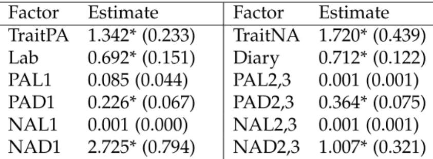
in the lab. Information curves and trace lines will then examined to determine if any

patterns exist in the same item across both methods and time points.

item. The solid lines represent the trace lines; whereas, the dotted lines represent

information. For the more desirable item, there is a high information curve across

θ with clear peaks; conversely, for the less desirable item there is low information

across a range of θ values. Thus, the less desirable item is not very informative

of an individual’s trait level. Secondly, the less desirable item does not have well

separated trace lines. This is problematic because there is not much variation in

response categories across different levels of θ. Ideally, a desirable item is one with

trace lines that discriminate well between categories; that is, trace lines that provide

good separation across different levels of θ.

(a) (b)

Figure 2.1: Example of (a) a“more desirable” item and (b) a “less desirable” item.

2.2.3 Longitudinal M-TSM Model for the PANAS Data

The proposed model consists of data from three time points. For each time point,

there are four latent state factors of interest, including PA lab, PA diary, NA lab and

NA diary. These state factors correspond to the participants’ momentary positive

affect and negative affect when assessed in a diary versus lab setting. Furthermore, it

is assumed that there are higher-order shared sources of variance in the participants’

shared sources of variances can be regarded as higher-order trait factors that capture

stable interindividual differences in overall levels of PA and NA. These trait factors,

denoted herein as PA trait and NA trait factors, are second-order factors that capture

systematic individual differences that are shared across time as well as method

set-tings. It is important to note that the residual variance of the state factors represents

what is common to all the items at a particular occasion and not carried to the next

time point. Whereas, the trait variance represents what is common to all the items

across time and setting. The trait-state representation is much like the trait-state

model proposed by Kenny and Zautra (2001).

The proposed model consists of a measurement model and a structural model.

The measurement model for the ordinal responses is

y_it∗ =µ+Λyη_it+εit (2.1)

where y∗_it is a p × 1 vector of unobserved continuous response variables for person

i at time t, Λy is a p × m factor loading matrix, η_it is an m × 1 vector of latent

endogenous variables for person iat time t, andεit is a p ×1 vector of measurement

errors.

Thejth unobserved continuous response variablesy∗_j,itis linked to thejth ordinal

manifest variablesyj,it by

yj,it =kif τj,k−1 <y∗j,it ≤τj,k (2.2)

whereτj,k are threshold parameters.

Finally, the structural part of the model involves a VARMA process at the latent

level. First introduced by Browne et Nesselroade (2005) with the name process factor

analysis model, the process considered differs from conventional VARMA processes

time. The model proposed in this thesis expands the process factor analysis model

by explicitly including a vector of second-order trait factors, yielding

η_it =Ληtraiti+A1ηi,t−1+A2ηi,t−2+...+Arηi,t−r+ζit (2.3)

where η_it is 6 × 1 vector of latent endogenous variables for person i at time t

consisting of the state factors: PA lab at time t, PA diary at time t, NA lab at time

t, NA diary at time t, lab at time t and diary at time t; traiti denotes a vector of

trait factor scores for person i. In the present application, these trait factors include

positive and negative affect at the trait level (i.e., second-order factors). Λη is a factor

loading matrix linking a vector of trait factors for person i to the state factors of all

time points. ζ_itis a vector of random shocks andA1, . . .,Arare autoregressive weight

matrices. The vector of second-order trait factors,traiti, is normally distributed with

zero means and variancesσ_ζ2

P andσ

2

ζN, respectively, and covarianceϑPN. The loadings

of the trait factors on all state factors are constrained to be invariant across time to

reflect the time-invariant nature of the trait factors.

Figure 2.2 shows a path diagram representation of the basic proposed model.

This proposed model contains repeated measures (over three time points) of the

positive and the negative affect items from the PANAS identified in the item-level

analysis. The model shown in Figure 2.2 features three lab and three diary factors

corresponding to the three repeated measurement occasions. Only the lag-one

au-toregression (e.g., from PAL1 to PAL2) but not the cross-regression (e.g., from PAL1 to

NAL2) paths are depicted in the path diagram. Whether the cross-regression paths

are needed will be evaluated as testable hypotheses. As mentioned, two trait

fac-tors, representing trait PA and trait NA, are specified to capture higher-order shared

valence effects among the first-order state affect factors. For instance, trait PA was

to load on all the state NA factors (NAL1-PAD3).

One issue of interest is the specification of identification constraints for the

lon-gitudinal M-TSM model. Within the time points, each state latent variable will be

specified to have the first factor loading set to one. Invariance constraints are

im-posed on the second-order factor loadings over time. This is because the trait factors

are purported to reflect constructs that are invariant and stable across time. In

addi-tion, the factor loadings of the trait factors on the lab-based state affect factors were

set to unity for identification purposes. The path diagram shown in Figure 2.2 shows

a model with these constraints specified for all time points. Whether this specific

set of constraints needs to be relaxed will be assessed in the model fitting process.

Furthermore, due to convergence issues with MTMM models, it might be necessary

to consider variations along the line of the correlated trait-correlated method minus

one model (Eid, 2000). In this case, loadings on a chosen reference method would

be constrained to be zero. The correlated trait-correlated uniqueness model (Kenny,

1976 ; Marsh, 1989), however, would be too restrictive for the proposed model

be-cause autoregressive paths between method factors would not be allowed. Thus, this

specific variation will not be considered.

A series of models will be fit in order to determine the final M-TSM model. First,

an examination of longitudinal invariance in the factor loadings and thresholds will

be performed. This is important because if invariance cannot be established, that

in-troduces added confounds and issues of change cannot be examined as readily.

Fur-thermore, invariance in the intercepts of the state factors will also be examined. In

the model shown in Figure 2.2, the intercepts of all state factors were set to zero.

De-viations of these intercepts from zero may indicate the existence of over-time trends

in the state factors, which could lead to spurious interpretations of other time series

parameters. Thus, as part of the invariance analysis, the intercepts of the state

...

...

...

...

...

...

...

...

...

...

...

...

...

...

...

...

φPD2

1

1

λP4L1

P

A

_L

1

λP4L2

PA

_L

2

λP4L3

P

A

_L3

λP4D1

P

A

_D

1

λP4D2

P

A

_D

2

λP4D3

P A _D 3 La b1 φD21

ζPL1

σ

2

φPD3

2

φPL2

1

φPL3

2

Tr

ait _PA

ζPL2

σ

2

ζPL3

σ

2

ζPD1

σ

2

ζPD2

σ

2

ζPD3

σ 2 1 1 1 λPD1 λPD2

λPD3

...

...

...

...

...

...

...

...

...

...

...

...

...

...

...

...

λN4L1

NA

_L1

λN4L2

NA

_L2

λN4L3

NA

_L3

λN4D1

NA

_D1

λN4D2

NA

_D2

λN4D3

NA _D3 ζNL1 σ 2 φND 32 φNL 21 φNL 32 Tr ait _NA ζNL2 σ 2 ζNL3 σ 2 ζND1 σ 2 ζND2 σ 2 ζND3 σ 2 1 1 1 λND1 λND2 λND3 Lab2 La b3 Di ar y1 Di ar y2 Di ar y3 1 1 1

λL3P4

1

λD1P 4

1

λD1P 4

1

λD3P4

λ L1 N1 λ L1 N4 λ L2 N1 λ L2 N4 λ L3 N1 λ L3 N4 λ D1 N4 λ D2 N4 λ D3 N4 λ D3 N1 λ D2 N1 λ D1 N1

λL1P 4 λL2P 4 φD32 φL21 φL32 ϑPN ζP σ 2 ζN σ 2 ζD3 σ 2 ζD2 σ 2 ζD1 σ 2 ζL3 σ 2 ζL2 σ 2 ζL1 σ 2 1 1 1 1 1 1 1 1 1 1 1

Figure 2.2: Path diagram of a longitudinal M-TSM model with VAR(1) relationships at the factor level. PA Mt = Positive Affect for method m at time t, NA Mt = Negative Affect for method M at time t, Labt = Lab at time t and Diaryt = Diary at time t. The factor loadings for the state factors are represented by ΛAtMt where A = Positive or

Negative Affect, M = Diary or Trait, and t is the time point. Likewise, the factor loading for the “method” factors are represented by λMtAt. The trait factor loadings

are represented by ΛAMt. The arrows depicted here correspond to elements in Λ

time points will be freed to evaluate the possible existence of trends. Secondly,

var-ious models with different time series structures will be considered. Finally, perfect

stability within the method factor will be tested.

Examining Longitudinal Invariance. The general procedure will be to begin with

a model with the least invariance constraints (namely, the model shown in Figure

2.2 wherein all factor loadings and thresholds are freed). Two models that were

nested within the first model will be then considered sequentially, with different

invariance constraints imposed. A summary of these models is shown in Table 2.1.

As mentioned, two types of invariance are of interest: configural and metric. The

goal of the invariance analysis is to retain items that at least display configural, or

preferably, metric invariance. As shown in Table 2.1, invariance constraints will be

sequentially imposed on the factor loadings followed by the thresholds.

In structural equation models involving continuous data, likelihood ratio tests

are often use to assess the relative fit of nested models (Bollen, 1989). However, when

categorical data are used with estimation methods such as the weighted least squares

means and variance adjusted (WLSMV) estimation (as will be used in the present

thesis), the differences in chi-square values between nested models are not chi-square

distributed. To adjust for this, the scaled chi-square difference test proposed by

Satorra and colleague (Satorra & Bentler, 1999 ; Satorra, 2000 ; Satorra & Bentler,

2010), as implemented in the DIFFTEST option in Mplus (Asparouhov & Muth´en,

2006), is used to examine changes in fit functions between models.

Table 2.1: Models Used to Examine Longitudinal Invariance in the PANAS Items.

Model 1 Free loadings, free thresholds Model 2 Invariant loadings, free thresholds Model 3 Invariant loadings, invariant thresholds

of a different specification of auto- and cross-regression structures. Autoregressive

paths will be specified for both the affect and the method factors (up to a lag order,r,

to be determined empirically by evaluating the statistical significance of high-order

autoregression parameters via Wald tests) to indicate the stability of these factors

over time; however, cross-regression paths will only be specified between the affect

factors. The models considered are: 1) a model with no auto-regression and no

cross-regression (denoted as the baseline model), 2) a model with only autoregressive paths

and no cross-regression and 3) a model with both auto- and cross-regression paths

of the optimal order.

I will then proceed to evaluating alternative models with further simplification

in the auto- and cross-regression structures. Four models will be considered for this.

The models will consist of a combination of a different number of lab and diary

factors. That is, the model will have either one factor representing all time points or

one factor for each time point. The models considered are: 1) one lab, one diary, 2)

one lab, three diary, 3) three lab, one diary and 4) three lab, three diary.

The justification for one factor verses three is testing for perfect stability. That

is, if a one-factor model is chosen over a three-factor model, then there is perfectly

stability over time for that factor, i.e. individuals’ factor scores at a later time point are

identical to their factor scores from earlier time points. Given the close proximity of

time points in both the lab and diary, perfect stability should be tested. It is possible

to constrain the one-factor models to be nested within the three-factor models. To

illustrate this, consider a model with no trait factor and only the method factors. In

this case, Model (1) is nested within Model (2); they are equivalent if the following

conditions are met in Model (2): (1) longitudinal invariance constraints are imposed

on the factor loadings, item thresholds, measurement error variances, (2) there are

no cross-regression paths and only lag-1 auto-regression paths are retained, (3) the

from time 2 to time 3 are constrained to be unity, and (3) the diary factor residual

variances at time 2 and time 3 are specified to be zero. Thus, likelihood ratio tests

can, in principle, be performed on nested models with appropriate constraints to test

the over-time stability of the method factors. However, due to the complexity of the

factor structures in the proposed longitudinal M-TSM model when cross-loadings on

the trait factors are present, other fit indices such as the RMSEA, CFI and TLI will be

CHAPTER 3

Results

The results section is organized as follows: 1) I will discuss results from the

IRT analyses, 2) results for examining longitudinal invariance will be presented, 3)

time series results and model testing concerning the stability of the state factors will

be discussed and 4) substantive findings and implications will be discussed in the

context of the final model.

3.1 Results for Item Analysis

3.1.1 IRT Analyses

The PANAS contains a total of 20 items; however, three items were not

mea-sured in the laboratory portion of the study (“afraid,” “hostile,” “excited”). These

items were therefore excluded in all subsequent analyses. Twelve univariate graded

response models were run in order to access item properties. The primary reason

for removing an item was because of low information. In other words, that item did

not measure an individual’s trait level on positive or negative affect very well. Issues

with poor trace line separation were also found; that is, there was not enough

vari-ation in response categories (see Figure 2.1). Finally, the χ2 LD statistic was used to

remove any items that displayed local dependence using a cutoff score of 10 (Chen

& Thissen, 1997). The final list of items retained is shown in Table 3.1. The reduced

set of items was found to yield interpretable factor loading and threshold structures.

Table 3.1: Final List of PANAS Items Retained.

Positive Affect Negative Affect

Active Ashamed

Attentive Distressed

Inspired Irritable

Strong Jittery

the PANAS was based (Zevon & Tellegen, 1982). In fact, only “active” and “strong”

overlap within the same content area; therefore, these eight items cover seven of the

20 content areas.

3.1.2 Establishing Longitudinal Invariance

Following the steps outlined in Table 2.1, the proposed model shown in Figure

2.2 was first fit with no invariance constraints on the loadings and thresholds. To aid

model convergence, I began by constraining all lag-one autoregressive parameters

and the residual variances to be invariant across time. Model fit indices indicate that

fit of the model was relatively poor (χ2(78) = 318.289, RMSEA = 0.114, CFI = 0.927

and TLI = 0.942). However, there was evidence suggesting configural invariance.

That is, all significant loadings had the same sign and relative magnitude. Some

of the residual variances were close to zero or negative and had to be constrained

to be greater than zero. As a result, I did not test for metric invariance formally

using a likelihood ratio test because the DIFFTEST option was not available with the

modeling constraints.1 Furthermore, the correlations between positive and negative

affect within lab were non-significant so those were constrained to be zero as well.

After invariance constraints were imposed on the factor loadings, a second model

with time-varying thresholds was considered. The thresholds were examined and

their magnitudes were found to be largely invariant across time. Figure 3.1 shows

1_{Models with time-varying time series parameters and time-varying residual variances were also}

the trace lines for “irritable” across time and method. As shown for this example

item, the general patterns of separation between trace lines were sustained across all

three assessment points. Other items considered were also observed to show similar,

largely invariant threshold structures over time.

Finally, invariance of the state factor intercepts and any potential deviations from

zero (i.e., an indication of the presence of trends) were examined. To do this, the

intercepts of the state affect factors at the second and third time points were allowed

to be freely estimated. Because there is no theoretical reason to assume systematic

trends in the method factors (lab and diary), the intercepts of the method factors

were kept at zero. Results showed that all estimated intercepts were non-significant;

therefore, no evidence for systematic mean change or trend was found.

The model from this section imposes invariance constraints on the factor loadings

and thresholds across time. Additionally, the model assumes all intercepts to be zero

across time and correlations within time were constrained to be zero between positive

and negative affect for state factors.

3.2 Most Parsimonious Model

This subsection presents the results from examining the time series structures of

the state affect factors and whether perfect stability can be established in the method

factors. The latter suggests that only one lab and one diary factor (or a combination)

is needed for all three time points. This indicates there is no additional uncertainty

from one time point to the next in the lab and diary setting. Emphasis will be placed

on interpreting the results corresponding to the final model.

To determine the order and structure of the VAR relations among the state affect

factors, Wald statistics were examined and any non-significant time series parameters

were set to zero. Because data were only available from three time points, the highest

lag order possible was a lag of two (i.e., a VAR(2) structure). Results indicated that

1 2

3 4

1 2

3 4

1

2

3 ₄

1

2 3

4

1

2 3 4

1

2 3

4

in the diary and positive affect in the lab, and lag-two autoregression parameters for

negative affect in the diary as well as positive affect in both the lab and diary.

Four models were fit to examine the hypothesis concerning perfect stability in the

methods factor. These models were treated as non-nested; the three method factors

were collapsed into one by creating one method factor. Table 3.2 shows fit indices for

the four models considered. There were no substantial changes in model fit between

the models so the most parsimonious model, namely, the one lab, one diary model,

was chosen. Furthermore, formulating the model with fewer method factors over

time as nested within the model with separate method factors at each time point led

to negligible changes in model fit and no difference in conclusions.

Table 3.2: Models Used to Examine Perfect Stability in the Method Factors

Model RMSEA CFI TLI Chi-square

Three lab, three diary 0.112 0.926 0.945 326.086 (df=83) Three lab, one diary 0.111 0.927 0.945 324.612 (df=83) One lab, three diary 0.112 0.927 0.945 325.855 (df=83) One lab, one diary 0.112 0.926 0.945 326.081 (df=83)

Note: The degrees of freedom (dfs) for all four models were the same despite the specification of fewer factors and the omission of autoregressive parameters for the method factors in the less complicated model. This was because when WLSMV estimation is used, the df has to be estimated and not just based on the difference in the number of parameters (Muth´en & Muth´en, 1998–2007).

Table 3.3 presents the parameter estimates obtained from the most parsimonious

model. The most parsimonious model consists of one lab and one diary factor and

all statistically significant parameters. Model fit indices indicate that fit of the final

model was not great by conventional standards (χ2(83) = 326.081, RMSEA = 0.112,

CFI = 0.926 and TLI = 0.945). However, the poor fit can be understood since slight

modeling discrepancies at various levels (e.g., mild violations of longitudinal

invari-ance assumptions on the threshold parameters) can compound into large reduction

T able 3.3: Factor Loadings for the Most Parsimonious Model Item P A Lab a P A Diar y NA Lab NA Diar y Lab b Diar y Activ e 1.000 1.000 Attentiv e 0.736* (0.084) -0.222* (0.090) Inspir ed 1.322* (0.106) 0.973* (0.111) Str ong 2.270* (0.216) -0.635* (0.273) Ashamed 1.000 -1.896* (0.235) Distr essed 0.835* (0.107) -0.445* (0.106) Irritable 0.833* (0.130) 0.128 (0.102) Jitter y 1.090* (0.192) 0.865* (0.194) Activ e 1.000 1.000 Attentiv e 1.215* (0.175) 1.087* (0.106) Inspir ed 1.161* (0.202) 1.738* (0.188) Str ong 1.417* (0.210) 1.045* (0.115) Ashamed 1.000 0.507* (0.207) Distr essed 0.696* (0.101) 0.131 (0.132) Irritable 0.655* (0.096) 0.046 (0.110) Jitter y 0.923* (0.145) 0.311 (0.160) Method T rait P A c T rait NA P A Lab 1.00 P A Diar y 0.473* (0.076) NA Lab 1.00 NA Diar y 0.214* (0.061) a State factor loadings for P A Diar y, P A Lab, NA Diar y and NA Lab ar e repr esented b y λA tM t in Figur e 2.2, wher e A = Positiv e or Negativ e Af fect, M = Diar y or T rait, and t is the time point. b Method factor loadings for lab and diar y ar e repr esented b y λM tA t in Figur e 2.2.

c Trait

whether conventional standards for approximate good fit are applicable to models

with categorical data.

The loadings for the state affect factors are all positive and high. This indicates

a well-defined factor structure for the state affect factors. The factor loading patterns

for the diary factor was also relatively clean. However, three of the factor loadings

for negative items were not significantly different from zero in the diary factor. This

suggests that these items did not contribute significantly to explaining the variance

in the diary factor.

A mixed pattern of factor loadings was observed for the lab factor. The general

pattern holds even when invariance constraints were not imposed on the loadings.

For instance, individuals responding in higher categories of “inspired” are

respond-ing to lower categories of “attentive” and “strong.” This illustrates the complexity

of affective responses that arose in the lab setting. The affect induction procedures

in the lab (emotion disclosure sections and negative slide shows) might have led to

particularly intense and mixed affective responses that did not all show the same

lev-els of continuity over time, as captured by the autoregressive parameters of the state

affect factors. Some of these lingering affective reactions were picked up by the lab

factor, leading to loadings of opposite signs between some of the PA and NA items.

As mentioned, covariances between positive and negative affect within each time

point were found to be nonsignificant; whereas, the covariance between positive and

negative affect at the trait level was -0.48 (corresponding to a correlation of -0.32).

Watson, Clark and Tellegen (1988) argued that positive and negative affects are

or-thogonal, i.e. with a zero covariance between the two. While that was found in the

state factors, the trait factors displayed a moderately negative covariance. This does

not conflict with previous research as other studies have found a moderately

nega-tive covariance between posinega-tive and neganega-tive affect in the PANAS (Feldman Barrett

indepen-dence while the trait factors do not. One possible explanation to this is that the trait

PA and trait NA are capturing low activation affective reactions, such as

happiness-sadness type of emotions, which Watson and Clark (1997) argued are inversely

re-lated. In contrast, the state PA and state NA might be getting at high activation

affective reactions, such as excitement-anger type of emotions, which would show

independence (Watson & Clark, 1997).

Table 3.4 shows the random shock variances from the most parsimonious model.

Of particular interest are the initial and residual variances for the state variables. The

initial variance represents the random shock variance at the first time point; whereas,

the residual variances are random shock variances after taking into account the effect

of previous time points via time series parameters. For both positive and negative

affect, the state factors in the diary setting have more random shock variance than

in the lab setting. That is, the diary setting has more fluctuations in random shocks

than the lab setting. Given the homogeneous nature of the experimental procedures

implemented across the three lab occasions, less within-person fluctuations in

pos-itive and negative affects can be expected across time in the lab setting. In fact the

study was designed such that participants viewed the slide show with comparable

negativity ratings at each time point; therefore, not as much variability would be

expected in emotions from one time point to the next. However, the emotion

induc-tion procedures could create some affective changes but such deviainduc-tions might have

diminished by the end of the negative slide shows.

Table 3.5 shows the time series parameter estimates for the most parsimonious

model; note that negative affect within the lab setting is excluded since there were no

significant autoregression parameters. The estimates of the autoregression

parame-ters suggested that both the PA and NA state fluctuations were stationary in nature2.

2_{That is, the eigenvalues of the transition matrix have moduli less than one or alternatively, all the}