Improved Differential-Linear Cryptanalysis
of 7-round Chaskey with Partitioning
Ga¨etan Leurent Inria, France
Abstract. In this work we study the security of Chaskey, a recent lightweight MAC designed by Mouhaet al., currently being considered for standardization by ISO/IEC and ITU-T. Chaskey uses an ARX structure very similar to SipHash. We present the first cryptanalysis of Chaskey in the single user setting, with a differential-linear attack against 6 and 7 rounds, hinting that the full version of Chaskey with 8 rounds has a rather small security margin. In response to these attacks, a 12-round version has been proposed by the designers.
To improve the complexity of the differential-linear cryptanalysis, we re-fine a partitioning technique recently proposed by Biham and Carmeli to improve the linear cryptanalysis of addition operations. We also propose an analogue improvement of differential cryptanalysis of addition opera-tions. Roughly speaking, these techniques reduce the data complexity of linear and differential attacks, at the cost of more processing time per data. It can be seen as the analogue for ARX ciphers of partial key guess and partial decryption for SBox-based ciphers.
When applied to the differential-linear attack against Chaskey, this par-titioning technique greatly reduces the data complexity, and this also results in a reduced time complexity. While a basic differential-linear attack on 7 round takes 278data and time (respectively 235for 6 rounds), the improved attack requires only 248 data and 267 time (respectively 225 data and 229time for 6 rounds). We also show an application of the partitioning technique to FEAL-8X, and we hope that this technique will lead to a better understanding of the security of ARX designs.
Keywords:Differential cryptanalysis, linear cryptanalysis, ARX, addi-tion, partitioning, Chaskey, FEAL
1
Introduction
Linear cryptanalysis and differential cryptanalysis are the two major cryptanalysis techniques in symmetric cryptography. Differential cryptanalysis was introduced by Biham and Shamir in 1990 [6], by studying the propagation of differences in a cipher. Linear cryptanalysis was discovered in 1992 by Matsui [29,28], using a linear approximation of the non-linear round function.
difference of the next round (resp. linear masks). The probability of the full differential or the imbalance of the full linear approximation is computed by multiplying the probabilities (respectively imbalances) of each round. This yields a statistical distinguisher for several rounds:
– A differential distinguisher is given by a plaintext differenceδP and a cipher-text differenceδC, so that the corresponding probabilitypis non-negligible:
p= PrE(P⊕δP) =E(P)⊕δC
2−n.
The attacker collects D = O(1/p) pairs of plaintexts (Pi, Pi0) with Pi0 =
Pi⊕δP, and checks whether a pair of corresponding ciphertexts satisfies
Ci0 =Ci⊕δC. This happens with high probability for the cipher, but with low probability for a random permutation.
– A linear distinguisher is given by a plaintext maskχP and a ciphertext mask
χC, so that the corresponding imbalance1εis non-negligible:
ε=2·Pr
P[χP]=C[χC]−1
2−n/2. The attacker collectsD=O(1/ε2) known plaintextsP
iand the corresponding ciphertextsCi, and computes the observed imbalance ˆε:
ˆ
ε=|2·#{i:Pi[χP] =Ci[χC]}/D−1|.
The observed imbalance is close to ε for the attacked cipher, and smaller than 1/√D (with high probability) for a random function.
Last round attacks. The distinguishers are usually extended to a key-recovery attack on a few more rounds using partial decryption. The main idea is to guess the subkeys of the last rounds, and to compute an intermediate state value from the ciphertext and the subkeys. This allows to apply the distinguisher on the intermediate value: if the subkey guess was correct the distinguisher should succeed, but it is expected to fail for wrong key guesses. In a Feistel cipher, the subkey for one round is usually much shorter than the master key, so that this attack recovers a partial key without considering the remaining bits. This allows a divide and conquer strategy were the remaining key bits are recovered by exhaustive search. For an SBox-based cipher, this technique can be applied if the differenceδC or the linear maskχC only affect a small number of SBoxes, because guessing the key bits affecting those SBoxes is sufficient to invert the last round.
ARX ciphers. In this paper we study the application of differential and linear cryptanalysis to ARX ciphers. ARX ciphers are a popular category of ciphers built using only additions (xy), bit rotations (x≪n), and bitwise xors (x⊕y). These simple operations are very efficient in software and in hardware, but they
1
interact in complex ways that make analysis difficult and is expected to provide security. ARX constructions have been used for block ciphers (e.g.TEA, XTEA, FEAL, Speck), stream ciphers (e.g.Salsa20, ChaCha), hash functions (e.g.Skein, BLAKE), and for MAC algorithms (e.g.SipHash, Chaskey).
The only non-linear operation in ARX ciphers is the modular addition. Its linear and differential properties are well understood [41,37,27,36,43,33,15], and differential and linear cryptanalysis have been use to analyze many ARX designs (see for instance the following papers: [4,45,44,24,25,18,8,29]).
However, there is no simple way to extend differential or linear distinguishers to last-round attack for ARX ciphers. The problem is that they typically have 32-bit or 64-bit words, but differential and linear characteristics have a few active bits in each word.2 Therefore a large portion of the key has to be guessed in order to perform partial decryption, and this doesn’t give efficient attacks.
Besides, differential and linear cryptanalysis usually reach a limited number of rounds in ARX designs because the trails diverge quickly and we don’t have good techniques to keep a low number of active bits. This should be contrasted with SBox-based designs where it is sometimes possible to build iterative trails, or trails with only a few active SBoxes per round. For instance, this is case for differential characteristics in DES [7] and linear trails in PRESENT [14].
Because of this, cryptanalysis methods that allow to divide a cipherE into two sub-ciphers E = E⊥◦E> are particularly interesting for the analysis of ARX designs. In particular this is the case with boomerang attacks [42] and differential-linear cryptanalysis [23,5]. A boomerang attack uses differentials with probabilities p> andp⊥ inE> andE⊥, to build a distinguisher with complexity O(1/p2>p2⊥). A differential-linear attack uses a differential with probabilitypfor
E> and a linear approximation with imbalanceεforE⊥ to build a distinguisher with complexity aboutO(1/p2ε4) (using a heuristic analysis).
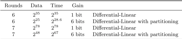
Table 1.Key-recovery attacks on Chaskey
Rounds Data Time Gain
6 235 235 1 bit Differential-Linear
6 225 228.6 6 bits Differential-Linear with partitioning
7 278 278 1 bit Differential-Linear
7 248 267 6 bits Differential-Linear with partitioning
Our results. In this paper, we consider improved techniques to attack ARX ciphers, with application to Chaskey. Since Chaskey has a strong diffusion, we start with differential-linear cryptanalysis, and we study in detail how to build a
2
good differential-linear distinguisher, and how to improve the attack with partial key guesses.
Our main technique follows a recent paper by Biham and Carmeli [3], by partitioning the available data according to some plaintext and ciphertext bits. In each subset, some data bits have a fixed value and we can combine this information with key bit guesses to deduce bits after the key addition. These known bits result in improved probabilities for differential and linear cryptanalysis. While Biham and Carmeli considered partitioning with a single control bit (i.e.two partitions), and only for linear cryptanalysis, we extend this analysis to multiple control bits, and also apply it to differential cryptanalysis.
When applied to differential and linear cryptanalysis, this results in a signifi-cant reduction of the data complexity. Alternatively, we can extend the attack to a larger number of rounds with the same data complexity. Those results are very similar to the effect of partial key guess and partial decryption in a last-round attack: we turn a distinguisher into a key recovery attack, and we can add some rounds to the distinguisher. While this can increase the time complexity in some cases, we show that the reduced data complexity usually leads to a reduced time complexity. In particular, we adapt a convolution technique used for linear cryptanalysis with partial key guesses [16] in the context of partitioning.
These techniques result in significant improvements over the basic linear technique: for 7 rounds of Chaskey (respectively 6 rounds), the differential-linear distinguisher requires 278 data and time (respectively 235), but this can be reduced to 248 data and 267 time (respectively 225 data and 229 time) (see Table 1). The full version of Chaskey has 8 rounds, and is claimed to be secure against attacks with 248data and 280 time.
The paper is organized as follows: we first explain the partitioning technique for linear cryptanalysis in Section 2 and for differential cryptanalysis in Section 3. We discuss the time complexity of the attacks in Section 4. Then we demonstrate the application of this technique to the differential-linear cryptanalysis of Chaskey in Section 5. Finally, we show how to apply the partitioning technique to reduce the data complexity of linear cryptanalysis against FEAL-8X in Appendix A.
2
Linear Analysis of Addition
We first discuss linear cryptanalysis applied to addition operations, and the improvement using partitioning. We describe the linear approximations using linear masks; for instance an approximation forE is written as Pr
E(x)[χ0]=
x[χ]
= 1/2±ε/2 whereχandχ0 are the input and output linear masks (x[χ]
denotesx[χ1]⊕x[χ2]⊕ · · ·x[χ`], whereχ= (χ1, . . . χ`) andx[χi] is bitχi ofx), andε≥0 is the imbalance. We also denote the imbalance of a random variablex
We first study linear properties of the addition operation, and use an ARX cipherE as example. We denote the word size asw. We assume that the cipher starts with an xor key addition, and a modular addition of two state variables.3 We denote the remaining operations as E0, and we assume that we know a linear approximation (α, β, γ) E
0
−→(α0, β0, γ0) with imbalanceεforE0. We further assume that the masks are sparse, and don’t have adjacent active bits. Following previous works, the easier way to extend the linear approximation is to use the following masks for the addition:
(α⊕α1, α)−→ α. (1)
As shown in Figure 1, this gives the following linear approximation forE:
(α⊕α1, β⊕α, γ)−→E (α0, β0, γ0). (2) In order to explain our technique, we initially assume thatαhas a single active bit,i.e.α= 2i. We explain how to deal with several active bits in Section 2.3. If
i= 0, the approximation of the linear addition has imbalance 1, but for other values ofi, it is only 1/2 [43]. In the following we study the case i >0, where the linear approximation (2) forE has imbalanceε/2.
E0
x3[α0] y3[β0]
z3[γ0]
x2[α] y2[β]
z2[γ]
x0[α⊕α1]
y0[β⊕α]
z0[γ]
kx ky
kz
x1[α⊕α1] y1[β⊕α]
z1[γ]
Fig. 1.Linear attack against the first addition
3
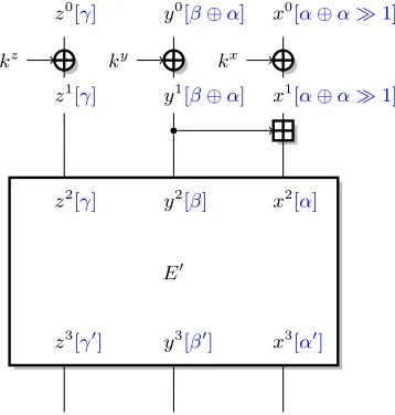
2.1 Improved analysis with partitioning
We now explain the improved analysis of Biham and Carmeli [3]. A simple way to understand their idea is to look at the carry bits in the addition. More precisely, we study an addition operations=ab, and we are interested in the values[α]. We assume thatα= 2i, i >0, and that we have some amount of input/output pairs. We denote individual bits ofaasa0, a1, . . . an−1, wherea0is the LSB (respectively,
biforbandsi fors). In addition, we consider the carry bitsci, defined asc0= 0,
ci+1= MAJ(ai, bi, ci) (where MAJ(a, b, c) = (a∧b)∨(b∧c)∨(c∧a)). Therefore, we havesi=ai⊕bi⊕ci.
Note that the classical approximationsi =ai⊕ai−1⊕bi holds with prob-ability 3/4 because ci = ai−1 with probability 3/4. In order to improve this approximation, Biham and Carmeli partition the data according to the value of bitsai−1andbi−1. This gives four subsets:
00 If (ai−1, bi−1) = (0,0), then ci= 0 and si=ai⊕bi.
01 If (ai−1, bi−1) = (0,1), then ε(ci) = 0 andε(si⊕ai⊕ai−1) = 0. 10 If (ai−1, bi−1) = (1,0), then ε(ci) = 0 andε(si⊕ai⊕ai−1) = 0. 11 If (ai−1, bi−1) = (1,1), then ci= 1 and si=ai⊕bi⊕1.
If bits ofaandbare known, filtering the data in subsets00and11gives a trail for the addition with imbalance 1 over one half of the data, rather than imbalance 1/2 over the full data-set. This can be further simplified to the following:
si=ai⊕bi⊕ai−1 ifai−1=bi−1 (3) In order to apply this analysis to the setting of Figure 1, we guess the key bitskxi−1 andkyi−1, so that we can compute the values ofx1i−1 andy1i−1 fromx0
andy0. More precisely, an attack onE can be performed with a single (logical) key bit guess, using Eq. (3):
x2i =x1i ⊕y1i ⊕xi1−1 ifx1i−1=yi1−1
x2i =x0i ⊕y0i ⊕x0i−1⊕kix⊕kiy⊕kxi−1 ifx0i−1⊕y0i−1=kxi−1⊕kiy−1
If we guess the key bitkxi−1⊕kyi−1, we can filter the data satisfyingx0i−1⊕yi0−1=
kxi−1 ⊕kyi−1, and we have ε(xi2⊕x0i ⊕yi0⊕x0i−1) = 1. Therefore the linear approximation (2) has imbalanceε. We need 1/ε2 data after the filtering for the attack to succeed,i.e.2/ε2 in total. The time complexity is also 2/ε2because we run the analysis with 1/ε2 data for each key guess. This is an improvement over a simple linear attack using (2) with imbalanceε/2, with 4/ε2 data.
Complexity. In general this partitioning technique multiply the data and time complexity by the following ratio:
RDlin= µ −1/
e
ε2 1/ε2 =ε
2/µ e
ε2 RTlin= 2 κ/
e
ε2 1/ε2 = 2
κε2/ e
ε2 (4) whereµis the fraction of data used in the attack, κis the number of guessed key bits,εis the initial imbalance, andεeis the improved imbalance for the selected subset. For Biham and Carmeli’s attack, we have µ= 1/2, κ= 1 and εe= 2ε, henceRD
2.2 Generalized partitioning
? ai0 ? ? + ? bi0 ? ? ? si? ? ?
0
? ai1 ? ? + ? bi1 ? ? ? si? ? ?
1
? ai0 0 ? + ? bi1 0 ? ? si? ? ?
0 0
? ai0 1 ? + ? bi1 1 ? ? si? ? ?
1 1
? ai1 0 ? + ? bi0 1 ? ? si? ? ?
? ?
Fig. 2.Some cases of partitioning for linear cryptanalysis of an addition
We now refine the technique of Biham and Carmeli using several control bits. In particular, we analyze cases01and10with extra control bitsai−2andbi−2 (some of the cases of shown in Figure 2):
01.00 If (ai−1, bi−1, ai−2, bi−2) = (0,1,0,0), thenci−1= 0, ci= 0 and si=ai⊕bi. 01.01 If (ai−1, bi−1, ai−2, bi−2) = (0,1,0,1),
thenε(ci−1) = 0,ε(ci) = 0, andε(si⊕ai⊕ai−1) = 0. 01.10 If (ai−1, bi−1, ai−2, bi−2) = (0,1,1,0),
thenε(ci−1) = 0,ε(ci) = 0, andε(si⊕ai⊕ai−1) = 0. 01.11 If (ai−1, bi−1, ai−2, bi−2) = (0,1,1,1),
thenci−1= 1, ci= 1 and si=ai⊕bi⊕1. 10.00 If (ai−1, bi−1, ai−2, bi−2) = (1,0,0,0),
thenci−1= 0, ci= 0 and si=ai⊕bi. 10.01 If (ai−1, bi−1, ai−2, bi−2) = (1,0,0,1),
thenε(ci−1) = 0,ε(ci) = 0, andε(si⊕ai⊕ai−1) = 0. 10.10 If (ai−1, bi−1, ai−2, bi−2) = (1,0,1,0),
thenε(ci−1) = 0,ε(ci) = 0, andε(si⊕ai⊕ai−1) = 0. 10.11 If (ai−1, bi−1, ai−2, bi−2) = (1,0,1,1),
thenci−1= 1, ci= 1 and si=ai⊕bi⊕1.
This yields an improved partitioning because we now have a trail for the addition with imbalance 1 in 12 out of 16 subsets:00.00, 00.01, 00.10, 00.11, 01.00, 01.11, 10.00, 10.11, 11.00, 11.01, 11.10, 11.11. We can also simplify this case analysis:
si=
ai⊕bi⊕ai−1
ai⊕bi⊕ai−2
ifai−1=bi−1
ifai−16=bi−1 andai−2=bi−2
This gives an improved analysis ofE by guessing more key bits. More precisely we needkx
i−1⊕k y
i−1 andk x i−2⊕k
y
i−2, as shown below:
x2i =
x1i ⊕yi1⊕x1i−1 x1
i ⊕yi1⊕x1i−2
ifx1i−1=yi1−1
ifx1
i−16=yi1−1andx1i−2=yi1−2
x2i =
x0
i ⊕yi0⊕xi0−1⊕kxi ⊕k y i ⊕k
x i−1
x0
i ⊕yi0⊕xi0−2⊕kxi ⊕k y i ⊕k
x i−2
ifx0
i−1⊕yi0−1=kix−1⊕k y i−1 ifx0
i−1⊕yi0−16=kix−1⊕k y i−1 andx0
i−2⊕yi0−2=kix−2⊕k y i−2
ε(x2i ⊕x0i ⊕yi0⊕x0i−1) = 1 ifx0i−1⊕yi0−1=kix−1⊕k y i−1
ε(x2i ⊕x0i ⊕yi0⊕x0i−2) = 1
ifx0i−1⊕yi0−16=kix−1⊕kyi−1
andx0
i−2⊕yi0−2=kix−2⊕k y i−2
Since this analysis yields different input masks for different subsets of the data, we use an analysis following multiple linear cryptanalysis [9]. We first divide the data into four subsets, depending on the value ofx0
i−1⊕y0i−1 andx0i−2⊕yi0−2, and we compute the measured (signed) imbalance ˆI[s] of each subset. Then, for each guess of the key bitskx
i−1⊕k y
i−1, andkix−2⊕k y
i−2, we deduce the expected imbalance Ik[s] of each subset, and we compute the distance to the observed imbalance asP
s(ˆI[s]−Ik[s])
2. According to the analysis of Biryukov, De Canni`ere and Quisquater, the correct key is ranked first (with minimal distance) with high probability when usingO(1/c2) samples, wherec2=P
iIi2= P
iε2i is the capacity of the system of linear approximations. Since we use three approximations with imbalanceε, the capacity of the full system is 3ε2, and we need 1/3·1/ε2
data in each subset after partitioning,i.e.4/3·1/ε2in total.
Again, the complexity ratio of this analysis can be computed asRDlin =ε2/µεe2 RlinT = 2κε2/eε2 Withµ= 3/4 andeε= 2ε, we find:
RDlin= 1/3 RTlin= 1.
The same technique can be used to refine the partitioning further, and give a complexity ratio ofRD
lin= 1/4×2
κ/(2κ−1) when guessingκbits.
Time complexity. In general, the time complexity of this improved partitioning technique is the same as the time complexity as the basic attack (RT
lin = 1), because we have to repeat the analysis 4 times (for each key of the key bits) with one fourth of the amount of data. We describe some techniques to reduce the time complexity in Section 4.
2.3 Combining partitions
For more complex scenarios, we select the filtering bits assuming that the active bits don’t interact, and we evaluate experimentally the probability in each subset. We can further study the matrix of probabilities to detect (logical) bits with no or little effect on the total capacity in order to improve the complexity of the attack. This will be used for our applications in Section 5 and Appendix A.
3
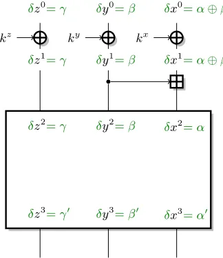
Differential Analysis of Addition
δx3=α0 δy3=β0
δz3=γ0
δx2=α δy2=β
δz2=γ
δx0=α⊕β
δy0=β
δz0=γ
kx
ky
kz
δx1=α⊕β δy1=β
δz1=γ
Fig. 3.Differential attack against the first addition
We now study differential properties of the addition. We perform our analysis in the same way as the analysis of Section 2, following Figure 3. We consider the first addition operation separately, and we assume that we know a differential (α, β, γ)→(α0, β0, γ0) with probabilitypfor the remaining of the cipher. Following previous works, a simple way to extend the differential is to linearize the first addition, yielding the following differences for the addition:
α⊕β, β−→ α.
3.1 Analysis of (α= 0, β= 2i)
Withi < w−1, the probability for the addition is Pr[(2i,2i)−→ 0] = 1/2.
Improved analysis with structures. We first discuss a technique using mul-tiple differentials and structures. More precisely, we use the following differentials for the addition:4
D1: (2i,2i)−→ 0 Prh(2i,2i)−→ 0i= 1/2
D2: (2i⊕2i+1,2i)−→ 0 Prh(2i⊕2i+1,2i)−→ 0i= 1/4
We can improve the probability ofD2 using a partitioning according to (ai, ai+1): 00 If (ai, ai+1) = (0,0), then a0=a2i2i+1 ands6=s0.
01 If (ai, ai+1) = (0,1), then a0=a2i and Pr[s=s0] = 1/2. 10 If (ai, ai+1) = (1,0), then a0=a2i and Pr[s=s0] = 1/2. 11 If (ai, ai+1) = (1,1), then a0=a2i2i+1 ands6=s0. This can be written as:
Prh(2i,2i)−→ 0i= 1/2
Prh(2i⊕2i+1,2i)−→ 0i= 1/2 ifai6=ai+1
The use of structures allows to build pairs of data for both differentials from the same data set. More precisely, we consider the following inputs:
p= (x0, y0, z0) q= (x0⊕2i, y0⊕2i, z0)
r= (x0⊕2i+1, y0, z0) s= (x0⊕2i+1⊕2i, y0⊕2i, z0)
We see that (p, q) and (r, s) follow the input difference ofD1, while (p, s) and (r, q) follow the input difference of D2. Moreover, we have from the partitioning:
Pr[E(p)⊕E(q) = (α0, β0, γ0)] = 1/2·p
Pr[E(r)⊕E(s) = (α0, β0, γ0)] = 1/2·p
Pr[E(p)⊕E(s) = (α0, β0, γ0)] = 1/2·p ifx0i ⊕x0i+16=kxi ⊕kxi+1 Pr[E(r)⊕E(q) = (α0, β0, γ0)] = 1/2·p ifx0i ⊕xi+10 =kxi ⊕kxi+1
For each key guess, we select three candidate pair out of a structure of four plain-texts, and every pair follows a differential forE with probabilityp/2. Therefore we need 2/ppairs, with a data complexity of 8/3·1/prather than 4·1/p.
In general this partitioning technique multiply the data and time complexity by the following ratio:
RdiffD = pe
−1T /(µT2/4)
p−1T /(T /2) = 2p
µTpe R
T diff= 2
κµRD diff=
2κ+1p
Tpe , (6)
4
whereµis the fraction of data used in the attack, κis the number of guessed key bits,T is the number of plaintexts in a structure (we considerT2/4 pairs rather thanT /2 without structures)pis the initial probability, andepis the improved probability for the selected subset. Here we have µ= 3/4,κ= 1,T = 4, and e
p=p, hence
RDdiff= 2/3 RdiffT = 1
Moreover, if the differential trail is used in a boomerang attack, or in a differential-linear attack, it impacts the complexity twice, but the involved key bits are the same, and we only need to use the structure once. Therefore, the complexity ratio should be evaluated as:
RDdiff-2=pe
−2T /(µT2/4)
p−2T /(T /2) = 2p2
µTpe2 R T diff-2= 2
κµRD diff-2=
2κ+1p2
Tpe2 , (7) In this scenario, we have the same ratios:
RDdiff-2= 2/3 RTdiff-2= 1
Generalized partitioning. We can refine the analysis of the addition by partitioning according to (bi). This gives the following:
Pr
(2i,2i)→0
= 1 ifai6=bi
Pr(2i⊕2i+1,2i)→0= 1 ifai=bi andai6=ai+1
This gives an attack withT = 4,µ= 3/8,κ= 2 andpe= 2p, which yield the same ratio in a simple differential setting, but a better ratio for a boomerang or differential-linear attack:
RDdiff= 2/3 RTdiff= 1
RDdiff-2= 1/3 RTdiff-2= 1/2
In addition, this analysis allows to recover an extra key bit, which can be useful for further steps of an attack.
Larger structure. Alternatively, we can use a larger structure to reduce the complexity: with a structure of size 2t, we have an attack with a ratioRD
diff= 1/2×2κ/(2κ−1), by guessingκ−1 key bits.
3.2 Analysis of (α= 2i, β= 0)
Improved analysis with structures. As in the previous section, we consider multiple differentials, and use partitioning to improve the probability:
D1: Prh(2i,0)−→ 2ii= 1/2
D2: Prh(2i⊕2i+1,0)−→ 2ii= 1/2 ifai6=ai+1
We also use structures in order to build pairs of data for both differentials from the same data set. More precisely, we consider the following inputs:
p= (x0, y0, z0) q= (x0⊕2i, y0, z0)
r= (x0⊕2i+1, y0, z0) s= (x0⊕2i+1⊕2i, y0, z0)
We see that (p, q) and (r, s) follow the input difference ofD1, while (p, s) and (r, q) follow the input difference of D2. Moreover, we have from the partitioning:
Pr[E(p)⊕E(q) = (α0, β0, γ0)] = 1/2·p
Pr[E(r)⊕E(s) = (α0, β0, γ0)] = 1/2·p
Pr[E(p)⊕E(s) = (α0, β0, γ0)] = 1/2·p ifx0i ⊕x0i+16=kxi ⊕kxi+1
Pr[E(r)⊕E(q) = (α0, β0, γ0)] = 1/2·p ifx0i ⊕xi+10 =kxi ⊕kxi+1
In this case, we also haveµ= 3/4,T = 4, andpe=p, hence
RDdiff= 2/3 RTdiff= 1
RDdiff-2= 2/3 RTdiff-2= 1
Generalized partitioning. Again, we can refine the analysis of the addition by partitioning according to (si). This gives the following:
Pr
(2i,0)→2i
= 1 ifai=si Pr
(2i⊕2i+1,0)→2i
= 1 ifai6=si andai6=ai+1
Since we can not readily filter according to bits ofs, we use the results of Section 2:
ai⊕bi⊕ai−1=si ifai−1=bi−1 This gives:
Pr
(2i,0)→2i
= 1 ifbi =ai−1andai−1=bi−1 Pr
(2i⊕2i+1,0)→2i
= 1 ifbi 6=ai−1andai−1=bi−1andai6=ai+1
Unfortunately, we can only use a small fraction of the pairsµ= 3/16. With
T = 4 and ep= 2p, this yields, an increase of the data complexity for a simple differential attack:
RDdiff= 4/3 RTdiff= 1/2
3.3 Analysis of (α= 2i, β= 2i)
Withi < w−1, the probability for the addition is Pr[(0,2i)−→ 2i] = 1/2. The results in this section will be the same as in the previous section, but we have to use a different structure. Indeed when this analysis is applied toE, we can freely modify the difference in x0 but not iny0, because it would affect the differential inE0.
More precisely, we use the following differentials:
D1: Prh(0,2i)−→ 2ii= 1/2
D2: Pr
h
(2i+1,2i)−→ 2ii= 1/2 ifai+16=bi and the following structure:
p= (x0, y0, z0) q= (x0, y0⊕2i, z0)
r= (x0⊕2i+1, y0, z0) s= (x0⊕2i+1, y0⊕2i, z0) This yields:
Pr[E(p)⊕E(q) = (α0, β0, γ0)] = 1/2·p
Pr[E(r)⊕E(s) = (α0, β0, γ0)] = 1/2·p
Pr[E(p)⊕E(s) = (α0, β0, γ0)] = 1/2·p ifx1i ⊕x0i+16=kyi ⊕ki+1x
Pr[E(r)⊕E(q) = (α0, β0, γ0)] = 1/2·p ifx1i ⊕xi+10 =kyi ⊕ki+1x
4
Improving the Time Complexity
The analysis of the previous sections assume that we repeat the distinguisher for each key guess, so that the data complexity is reduced in a very generic way. When this is applied to differential or linear cryptanalysis, it usually result in an increased time complexity (RT >1). However, when the distinguisher is a simple linear of differential distinguisher, we can perform the analysis in a more efficient way, using the same techniques that are used in attacks with partial key guess against SBox-based ciphers. For linear cryptanalysis, we use a variant of Matsui’s Algorithm 2 [28], and the improvement using convolution algorithm [16]; for differential cryptanalysis we filter out pairs that can not be a right pair for any key. In the best cases, the time complexity of the attacks can be reduced to essentially the data complexity.
4.1 Linear analysis
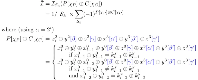
More precisely, let us explain this idea within the setting of Section 2.2 and Figure 1. For each key guess, the attacker computes the observed imbalance over a subsetSk corresponding to the data withx0i−1⊕y0i−1=kix−1⊕k
y i−1, or
x0i−1⊕yi0−1=6 kix−1⊕kyi−1 andxi0−2⊕yi0−2=kix−2⊕kyi−2: ˆ
I=ISk(P[χP]⊕C[χC])
= 1/|Sk| ×X
Sk
(−1)P[χP]⊕C[χC]
where (usingα= 2i)
P[χP]⊕C[χC] =x2i ⊕y
2[β]⊕z2[γ]⊕x3[α0]⊕y3[β0]⊕z3[γ0]
=
x0
i ⊕yi0⊕x0i−1⊕y0[β]⊕z0[γ]⊕x3[α0]⊕y3[β0]⊕z3[γ0] ifx0
i−1⊕yi0−1=kix−1⊕k y i−1
x0
i ⊕yi0⊕x0i−2⊕y0[β]⊕z0[γ]⊕x3[α0]⊕y3[β0]⊕z3[γ0] ifx0i−1⊕yi0−16=kix−1⊕kyi−1
andx0i−2⊕y0i−2=kxi−2⊕kyi−2
Therefore, the imbalance can be efficiently reconstructed from a series of 24 counters keeping track of the amount of data satisfying every possible value of the following bits:
x0i ⊕y0i ⊕x0i−1⊕y0[β]⊕z0[γ]⊕x3[α0]⊕y3[β0]⊕z3[γ0],
x0i−1⊕xi0−2, x0i−1⊕y0i−1, xi0−2⊕y0i−2
This results in an attack where the time complexity is equal to the data complexity, plus a small cost to compute the imbalance. The analysis phase require only about 26operations in this case (adding 24 counters for 22 key guesses). When the amount of data required is larger than 26, the analysis step is negligible.
When several partitions are combined (with several active bits in the first additions), the number of counters increases to 2b, wherebis the number of control bits. To reduce the complexity of the analysis phase, we can use a convolution algorithm (following [16]), so that the cost of the distillation is only O(b·2b) rather thanO(2κ·2b). This will be explained in more details with the application to Chaskey in Section 5.
In general, there is a trade-off between the number of partitioning bits, and the complexity. A more precise partitioning allows to reduce the data complexity, but this implies a larger set of counters, hence a larger memory complexity. When the number of partitioning bits reaches the data complexity, the analysis phase becomes the dominant phase, and the time complexity is larger than the data complexity.
4.2 Differential analysis
we use a simple differential distinguisher with output difference δ0, following Section 3 (whereδ0= (α0, β0, γ0))
We first define a linear functionLwith rankn−1 (wherenis the block size), so that L(δ0) = 0. In particular, any pairx, x0 =x⊕δ0 satisfies L(x) =L(x0). This allows to detect collisions by looking at allvaluesin a structure, rather than allpairs in a structure. We just compute L(E(x)) for allx’s in a structure, and we look for collisions.
5
Application to Chaskey
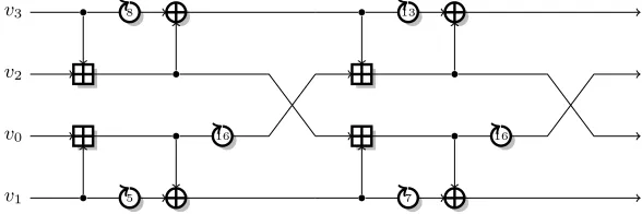
Chaskey is a recent MAC proposal designed jointly by researchers from COSIC and Hitachi [35]. The mode of operation of Chaskey is based on CBC-MAC with an Even-Mansour cipher; but it can also be described as a permutation-based design as seen in Figure 4. Chaskey is designed to be extremely fast on 32-bit micro-controllers, and the internal permutation follows an ARX construction with 4 32-bit words based on SipHash; it is depicted in Figure 5. Since the security of Chaskey is based on an Even-Mansour cipher, the security bound has a birthday termO(T D·2−128). More precisely, the designers claim that it should be secure up to 248 queries, and 280 computations.
K m0
π m1
π
m2 K0
π K0
τ
Fig. 4.Chaskey mode of operation (full block message)
v1
v0
v2
v3
5 8
16
7 13
16
Fig. 5.One round of the Chaskey permutation. The full permutation has 8 rounds.
extended into a 5 round attack following the method of attacks against the Salsa family[1]. It is important to try more advanced techniques in order to understand the security of Chaskey, in particular because it is being considered for standardization.
5.1 Differential-linear cryptanalysis
Table 2.Probabilities of the best differential characteristics of Chaskey reported by the designers [35]
Rounds: 1 2 3 4 5 6 7 8
Probability: 1 2−4 2−16 2−37 2−73.1 2−132.8 2−205.6 2−289.9
The best differential characteristics found by the designers of Chaskey quickly become unusable when the number of rounds increase (See Table 2). The designers also report that those characteristics have an “hourglass structure”: there is a position in the middle where a single bit is active, and this small difference is expanded by the avalanche effect when propagating in both direction. This is typical of ARX designs: short characteristics have a high probability, but after a few rounds the differences cannot be controlled and the probability decrease very fast. The same observation typically holds also for linear trails.
Because of these properties, attacks that can divide the cipherE in two parts
E =E⊥◦E> and build characteristics or trail for both half independently – such as the boomerang attack or differential-linear cryptanalysis – are partic-ularly interesting. In particular, many attacks on ARX designs are based on the boomerang attack [46,31,11,26,22,39] or differential-linear cryptanalysis [20]. Since Chaskey never uses the inverse permutation, we cannot apply a boomerang attack, and we focus on differential-linear cryptanalysis.
x
y
z E>
E⊥>
x0
y0
z0 E>
E⊥> δi
δo
χi
χo
χi
χo
Differential-linear cryptanalysis uses a differentialδi E>
−→δo with probability
pfor E>, and a linear approximationχi E⊥
−→χo with imbalance εfor E⊥ (see Figure 6). The attacker uses pairs of plaintexts (Pi, Pi0) with Pi0 = Pi ⊕δi, and computes the observed imbalance ˆε = |2·#{i:Ci[χo]=Ci0[χo]}/D−1|.
Following the heuristic analysis of [5], the expected imbalance is aboutpε2, which gives an attack complexity ofO(2/p2ε4):
– A pair of plaintext satisfiesE>(P)⊕E>(P0) =δowith probabilityp. In this case, we haveE>(P)[χi]⊕E>(P0)[χi]=δo[χi]. Without loss of generality,
we assume thatδo[χi]= 0.
– Otherwise, we expect thatE>(P)[χi]⊕E>(P0)[χi]is not biased. This gives
the following: Pr
E>(P)[χi]⊕E>(P0)[χi]= 0
=p+ (1−p)·1/2 = 1/2 +p/2 (8)
ε(E>(P)[χi]⊕E>(P0)[χi]) =p (9)
– We also haveε(E>(P)[χi]⊕C[χo]) =ε(E>(P0)[χi]⊕C0[χo]) =ε from the
linear approximations. Combining with (9), we getε(C[χo]⊕C0[χo]) =pε2.
A more rigorous analysis has been recently provided by Blondeau, Leander and Nyberg [13], but since we use experimental values to evaluate the complexity of our attacks, this heuristic explanation will be sufficient.
5.2 Using partitioning
A differential-linear distinguisher can easily be improved using the results of Section 2 and 3. We can improve the differential and linear part separately, and combine the improvements on the differential-linear attack. More precisely, we have to consider structures of plaintexts, and to guess some key bits in the differential and linear parts. We partition all the potential pairs in the structures according to the input difference, and to the filtering bits in the differential and linear part; then we evaluate the observed imbalance ˆI[s] in every subsets. Finally, for each key guessk, we compute the expected imbalanceIk[s] for each subsets, and then we evaluate the distance between the observed and expected imbalances asL(k) =P
s(ˆI[s]− Ik[s])2 (following the analysis of multiple linear cryptanalysis [10]).
While we follow the analysis of multiple linear cryptanalysis to evaluate the complexity of our attack, we use each linear approximation on a different subset of the data, partitioned according to the filtering bits. In particular, we don’t have to worry about the independence of the linear approximations.
If we use structures of size T, and select a fraction µdiff of the input pairs with an improved differential probability pe, and a fraction µlin of the output pairs with an improved linear imbalance eε, the data complexity of the attack is O(µlinµ2diffT /2×2/pe
2 e
ε4). This corresponds to a complexity ratio ofRDdiff-2RDlin2. More precisely, using differential filtering bitspdiff and linear filtering bits
and the cipher text bitsC[clin] and C0[clin], withC=E(P) andC0 =E(P⊕
∆). In practice, for everyP, P0 in a structure, we update the value of ˆI[P⊕
P0, P[plin], C[cdiff], C0[cdiff]].
We also take advantage of the Even-Mansour construction of Chaskey, without keys inside the permutation. Indeed, the filtering bits used to define the subsetss
correspond to the key bits used in the attack. Therefore, we only need to compute the expected imbalance for the zero key, and we can deduce the expected imbalance for an arbitrary key asIkdiff,klin[∆, p, c, c
0] =I0[∆, p⊕k
lin, c⊕kdiff, c0⊕kdiff].
Time complexity. This description lead to an attack with low time complexity using an FFT algorithm, as described previously for linear cryptanalysis [16] and multiple linear cryptanalysis [19]. Indeed, the distance between the observed and expected imbalance can be written as:
L(k) =X s
(ˆI[s]− Ik[s])2
=X
s
(ˆI[s]− I0[s⊕φ(k)])2, where φ(kdiff, klin) = (0, klin, kdiff, kdiff)
=X
s ˆ
I[s]2+X s
I0[s⊕φ(k)]2−2X s
ˆ
I[s]I0[s⊕φ(k)],
where only the last term depend on the key. Moreover, this term can be seem as theφ(k)-th component of the convolutionI0∗Iˆ. Using the convolution theorem, we can compute the convolution efficiently with an FFT algorithm.
This gives the following fast analysis:
1. Compute the expected imbalanceI0[s] of the differential-linear distinguisher for the zero key, for every subsets.
2. CollectD plaintext-ciphertext pairs, and compute the observed imbalance ˆ
I[s] of each subset.
3. Compute the convolutionI ∗Iˆ, and findkthat maximizes coefficientφ(k).
5.3 Differential-linear Cryptanalysis of Chaskey
In order to find good differential-linear distinguishers for Chaskey, we use a heuristic approach. We know that most good differential characteristics and good linear trails have an “hourglass structure”, with a single active bit in the middle. If a good differential-linear characteristics is given with this “hourglass structure”, we can divideEin three partsE=E⊥◦E⊥>◦E>, so that the single active bit in the differential characteristic falls betweenE> andE⊥>, and the single active bit in the linear trail falls betweenE⊥> andE⊥. We use this decomposition to look for good differential-linear characteristics: we first divideE in three parts, and we look for a differential characteristicδi
E>
−→δo inE> (with probabilityp), a differential-linear characteristicδo
E⊥>
−→χi inE⊥> (with imbalanceb), and a linear characteristicχi
E⊥
active bit. This gives a differential-linear distinguisher with imbalance close to
bpε2:
– We consider a pair of plaintext (P, P0) withP0 = P⊕δi, and we denote
X=E>(P),Y =E>⊥(X),C=E⊥(Y).
– We haveX⊕X0=δo with probabilityp. In this case,ε(Y[χi]⊕Y0[χi]) =b
– Otherwise, we expect thatY[χi]⊕Y0[χi]is not biased. This gives the following:
Pr
Y[χi]⊕Y0[χi]= 0
= (1−p)·1/2 +p·(1/2 +b/2) = 1/2 +bp/2 (10)
ε(Y[χi]⊕Y0[χi]) =bp (11)
– We also have ε(Y[χi]⊕C[χo]) = ε(Y0[χi]⊕C0[χo]) = ε from the linear
approximations. Combining with (11), we getε(C[χo]⊕C0[χo]) =bpε2.
In theE⊥> section, we can see the characteristic as a small differential-linear characteristic with a single active input bit and a single active output bit, or as a truncated differential where the input difference has a single active bit and the output value is truncated to a single bit. In other words, we use pairs of values with a single bit difference, and we look for a biased output bit difference.
We ran an exhaustive search over all possible decompositionsE =E⊥◦E⊥>◦E> (varying the number of rounds), and all possible positions for the active bitsiat the input ofE⊥> and the biased bit5 j at the output of E⊥>. For each candidate, we evaluate experimentally the imbalanceε(E⊥>(x)[j]⊕E⊥>(x⊕2i)[j]), and we study the best differential and linear trails to build the full differential-linear distinguisher. This method is similar to the analysis of the Salsa family by Aumassonet al.[1]: they decompose the cipher in two partsE =E⊥◦E⊥>, in order to combine a biased bit inE⊥> with an approximation ofE⊥.
This approach allows to identify good differential-linear distinguisher more easily than by building full differential and linear trails. In particular, we avoid most of the heuristic problems in the analysis of differential-linear distinguish-ers (such as the presence of multiple good trails in the middle) by evaluating experimentally ε(E⊥>(x)[j]⊕E⊥>(x⊕2i)[j]) without looking for explicit trails in the middle. In particular, the transition betweenE> and E⊥> is a transition between two differential characteristics, while the transition betweenE⊥>andE⊥ is a transition between two linear characteristics.
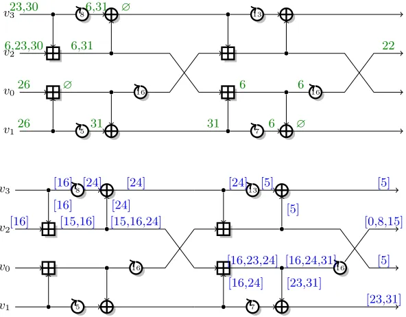
5.4 Attack against 6-round Chaskey
The best distinguisher we identified for an attack against 6-round Chaskey uses 1 round inE>, 4 rounds inE⊥>, and 1 round in E⊥. The optimal differences and masks are:
– Differential forE> with probability p> ≈2−5:
v0[26], v1[26], v2[6,23,30], v3[23,30] E>
−→v2[22]
5
v1 v0 v2 v3 5 8 16 7 13 16 22 6 ∅ 6 6 31 31 ∅ 6,31 6,31 ∅ 26 26 6,23,30 23,30 v1 v0 v2 v3 5 8 16 7 13 16 [23,31] [5] [0,8,15] [5] [5] [5] [24] [24] [24] [16] [16] [16,24,31] [16,24] [16,23,24] [23,31] [15,16] [15,16,24] [24] [16]
Fig. 7.6-round attack: differential characteristic, and linear trail.
– Biased bit forE⊥> with imbalanceε⊥>= 2−6.05:
v2[22] E⊥>
−→v2[16]
– Linear approximations forE⊥ with imbalanceε⊥= 2−2.6:
v2[16] E⊥
−→v0[5], v1[23,31], v2[0,8,15], v3[5] The differential and linear trails are shown in Figure 7. The expected imbalance is
p>·ε⊥>·ε2⊥ = 2−16.25. This gives a differential-linear distinguisher with expected complexity in the order ofD= 2/p2>ε>⊥2ε4⊥≈233.5.
We can estimate the data complexity more accurately using [12, Eq. (11)]: we need about 234.1pairs of samples in order to reach a false positive rate of 2−4. Experimentally, with 234pairs of samples (i.e.235data), the measured imbalance is larger than 2−16.25with probability 0.5; with random data, it is larger than 2−16.25 with probability 0.1. This matches the predictions of [12], and confirms the validity of our differential-linear analysis.
This simple differential-linear attack is more efficient than generic attacks against the Even-Mansour construction of Chaskey. It follows the usage limit of Chaskey, and reaches more rounds than the analysis of the designers. Moreover, it we can be improved significantly using the results of Sections 2 and 3.
trail becomes:
v2[16] E⊥
−→v1[16,24], v2[16,23,24], v3[24]
We select control bits to improve the probability of the addition between v1 and v2on active bits 16 and 24. Following the analysis of Section 2.2, we need
v1[14]⊕v2[14] andv1[15]⊕v2[15] as control bits for active bit 16. To identify more complex control bits, we considerv1[14,15,22,23], v2[14,15,22,23] as potential control bits, as well asv3[23] because it can affect the addition on the previous half-round. Then, we evaluate the bias experimentally (using the round function as a black box) in order to remove redundant bits. This leads to the following 8 control bits:
v1[14]⊕v2[14] v1[14]⊕v1[15] v1[22] v1[23]
v1[15]⊕v2[15] v1[15]⊕v3[23] v2[22] v2[23]
This defines 28partitions of the ciphertexts, after guessing 8 key bits. We evaluated the bias in each partition, and we found that the combined capacity isc2= 26.84. This means that we have the following complexity ratio
RDlin= 2−2·2.6/2−826.84≈2−4 (12)
Analysis of differential with partitioning. There are four active bits in the first additions:
– Bit 23 inv2v3: (223,223)−→ 0 – Bit 30 inv2v3: (230,230)−→ 231 – Bit 6 inv2v3: (26,0)−→ 26 – Bit 26 inv0v1: (226,226)−→ 0
Following the analysis of Section 3, we can use additional input differences for each of them. However, we reach a better trade-off by selected only three of them. More precisely, we consider 23 input differences, defined byδ
i and the following extra active bits:
v2[24] v2[31] v0[27]
As explained in Section 2, we build structures of 24 plaintexts, where each structure provides 23pairs for every input difference,i.e.26 pairs in total.
Following the analysis of Section 3, we use the following control bits to improve the probability of the differential:
v2[23]⊕v2[24] v2[30]⊕v3[30] v0[26]⊕v0[27]
v2[24]⊕v3[23] v0[27]⊕v1[26]
differentials. We found that, for 18 of those subsets, there is a probability 2−2 to reach δo (the probability is 0 for the remaining subsets). This leads to a complexity ratio:
RDdiff= 2·2 −5
18/28×24×2−2 = 2/9
RDdiff-2=
2·22×−5
18/28×24×22×−2 = 1/36
This corresponds to the analysis of Section 3: we have a ratio of 2/3 for bits
v2[23] andv0[27] (Section 3.1), and a ratio of 1/2 for v2[31] in the simple linear case. In the differential-linear case, we have respectively ratios of 1/3 and 1/4.
Finally, the improved attack requires a data complexity in the order of:
RDlin2RDdiff-2D≈220.3.
We can estimate the data complexity more accurately using the analysis of Biryukov, De Canni`ere and Quisquater [9]. First, we give an alternate description of the attack similar the multiple linear attack framework. Starting fromDchosen plaintexts, we build 22Dpairs using structures, and we keepN = 18·2−8·2−14·22D samples per approximation after partitioning the differential and linear parts. The imbalance of the distinguisher is 2−2·2−6.05·26.84 = 2−1.21. Following [9, Corollary 1], the gain of the attack withD= 224is estimated as 6.6 bits,i.e.the average key rank should be about 42 (for the 13-bit subkey).
Using the FFT method of Section 5.2, we perform the attack with 224 counters ˆI[s]. Each structure of 24 plaintexts provides 26 pairs, so that we need 22D operations to update the counters. Finally, the FFT computation require 24×224≈228.6operations.
We have implemented this analysis, and it runs in about 10s on a single core of a desktop PC.6 Experimentally, we have a gain of about 6 bits (average key rank of 64 with 128 experiments); this validates our theoretical analysis. We also notice some key bits don’t affect the distinguisher and cannot be recovered. On the other hand, the gain of the attack can be improved using more data, and further trade-offs are possible using larger or smaller partitions.
5.5 Attack against 7-round Chaskey
The best distinguisher we identified for an attack against 7-round Chaskey uses 1.5 round in E>, 4 rounds inE⊥>, and 1.5 round inE⊥. The optimal differences and masks are:
– Differential forE> with probability p> = 2−17:
v0[8,18,21,30], v1[8,13,21,26,30], v2[3,21,26], v3[21,26,27] E>
−→v0[31]
6
– Biased bit forE⊥> with imbalanceε⊥>= 2−6.1:
v0[31] E⊥>
−→v2[20]
– Linear approximations forE⊥ with imbalanceε⊥= 2−7.6:
v2[20] E⊥
−→v0[0,15,16,25,29], v1[7,11,19,26], v2[2,10,19,20,23,28], v3[0,25,29] This gives a differential-linear distinguisher with expected complexity in the order of D= 2/p2
>ε2⊥>ε4⊥≈277.6. This attack is more expensive than generic attacks against on the Even-Mansour cipher, but we now improve it using the results of Sections 2 and 3.
Analysis of linear approximations with partitioning. We use an automatic search to identify good control bits, starting from the bits suggested by the result of Section 2. We identified the following control bits:
v1[3]⊕v1[11]⊕v3[10] v1[3]⊕v1[11]⊕v3[11] v0[15]⊕v3[14]
v0[15]⊕v3[15] v1[11]⊕v1[18]⊕v3[17] v1[11]⊕v1[18]⊕v3[18]
v1[3]⊕v2[2] v1[3]⊕v2[3] v1[11]⊕v2[9]
v1[11]⊕v2[10] v1[11]⊕v2[11] v1[18]⊕v2[17]
v1[18]⊕v2[18] v1[2]⊕v1[3] v1[9]⊕v1[11]
v1[10]⊕v1[11] v1[17]⊕v1[18] v0[14]⊕v0[15]
v0[15]⊕v1[3]⊕v1[11]⊕v1[18]
Note that the control bits identified in Section 2 appear as linear combinations of those control bits.
This defines 219 partitions of the ciphertexts, after guessing 19 key bits. We evaluated the bias in each partition, and we found that the combined capacity is
c2= 214.38. This means that we gain the following factor:
RDlin= 2−2·7.6/2−19214.38≈2−10.5 (13) This example clearly shows the power of the partitioning technique: using a few key guesses, we essentially avoid the cost of the last layer of additions.
Analysis of differential with partitioning. We consider 29input differences, defined byδi and the following extra active bits:
v0[9] v0[22] v0[31] v0[19]
v0[14] v0[27] v2[22] v2[27] v2[4]
As explained in Section 2, we build structures of 210 plaintexts, where each structure provides 29pairs for every input difference,i.e.218 pairs in total.
probability of the differential:
v0[4]⊕v2[3] v2[22]⊕v3[21] v2[27]⊕v3[26] v2[27]⊕v3[27]
v2[3]⊕v2[4] v2[21]⊕v2[22] v2[26]⊕v2[27] v0[9]⊕v1[8]
v0[14]⊕v1[13] v0[27]⊕v1[26] v0[30]⊕v1[30] v0[8]⊕v0[9]
v0[18]⊕v0[19] v0[21]⊕v0[22]
This divides each set of pairs into 214 subsets, after guessing 14 key bits. In total we have 223 subsets to analyze, according to the control bits and the multiple differentials. We found that, for 17496 of those subsets, there is a probability 2−11to reachδ
o (the probability is 0 for the remaining subsets). This leads to a ratio:
Rdiff-2D = 2·2 −2·17
17496/223×210×2−2·11 = 1/4374≈2 −12.1
Finally, the improved attack requires a data complexity of:
RDlin2RDdiff-2D≈244.5.
Again, we can estimate the data complexity more accurately using [9]. In this attack, starting fromN0chosen plaintexts, we build 28N0pairs using structures, and we keep N = 17496·2−23·2−38·28N
0 samples per approximation after partitioning the differential and linear parts. The imbalance of the distinguisher is 2−11·2−6.1·214.38= 2−2.72. Following [9, Corollary 1], the gain of the attack withN0= 248 is estimated as 6.3 bits,i.e. the average rank of the 33-bit subkey should be about 225.7. Following the experimental results of Section 5.4, we expect this to estimation to be close to the real gain (the gain can also be increased if more than 248 data is available).
Using the FFT method of Section 5.2, we perform the attack with 261counters ˆ
I[s]. Each structure of 210 plaintexts provides 218 pairs, so that we need 28D
operations to update the counters. Finally, the FFT computation require 61× 261≈267 operations.
This attack recovers only a few bits of a 33-bit subkey, but an attacker can run the attack again with a different differential-linear distinguisher to recover other key bits. For instance, a rotated version of the distinguisher will have a complexity close to the optimal one, and the already known key bits can help reduce the complexity.
Conclusion
partitioning for differential cryptanalysis. This allows a significant reduction of the data complexity of attacks against ARX ciphers, and is particularly efficient with boomerang and differential-linear attacks.
Our main application is a differential-linear attack against Chaskey, that reaches 7 rounds out of 8. In this application, the partitioning technique allows to go through the first and last additions almost for free. This is very similar to the use of partial key guess and partial decryption for SBox-based ciphers. This is an important result because standard bodies (ISO/IEC JTC1 SC27 and ITU-T SG17) are currently considering Chaskey for standardization, but little external cryptanalysis has been published so far. After the first publications of these results, the designers of Chaskey have proposed to standardize a new version with 12 rounds [34].
Acknowledgement
We would like to thank Nicky Mouha for enriching discussions about those results, and the anonymous reviewers for their suggestions to improve the presentation of the paper.
A
Appendix: Application to FEAL-8X
We now present application of our techniques to reduce the data complexity of differential and linear attacks.
FEAL is an early block cipher proposed by Shimizu and Miyaguchi in 1987 [40]. FEAL uses only addition, rotation and xor operations, which makes it much more efficient than DES in software. FEAL has inspired the development of many cryptanalytic techniques, in particular linear cryptanalysis.
At the rump session of CRYPTO 2012, Matsui announced a challenge for low data complexity attacks on FEAL-8X using only known plaintexts. At the time, the best practical attack required 224 known plaintexts [2] (Matsui and Yamagishi had non-practical attacks with as little as 214 known plaintext [29]), but Biham and Carmeli won the challenge with a new linear attack using 215 known plaintexts, and introduced the partitioning technique to reduce the data complexity to 214[3]. Later Sakikoyamaet al.improved this result using multiple linear cryptanalysis, with a data complexity of only 212 [38].
We now explain how to apply the generalized partitioning to attack FEAL-8X. Our attack follows the attack of Biham and Carmeli [3], and uses the generalized partitioning technique to reduce the data complexity further. The attack by Biham and Carmeli requires 214data and about 245time, while our attack needs only 212data, and 245time. While the attack of Sakikoyamaet al.is more efficient with the same data complexity, this shows a simple example of application of the generalized partitioning technique.
partial decryption for the last round (with a 22 bit key guess). This allows to compute enough bits of the state after the first round and before the last round, respectively, to compute the linear approximation. For more details of the attack, we refer the reader to the description of Biham and Carmeli [3].
In order to improve the attack, we focus on the round function of the second-to-last round. The corresponding linear approximation isx[10115554]→
y[04031004] with imbalance of approximately 2−3.
We partition the data according to the following 4 bits7 (note that all those bits can be computed in the input of round 6 with the 22-bit key guess ofDK7):
b0=f0,3⊕f1,3⊕f2,2⊕f3,2 b1=f0,3⊕f1,3⊕f2,3⊕f3,3
b2=f0,3⊕f1,3⊕f2,5⊕f3,5 b3=f0,2⊕f1,2⊕f0,3⊕f1,3
The probability of the linear approximation in each subset is as follows (indexed by the value ofb3, b2, b1, b0):
p0000= 0.250 p0001= 0.270 p0010= 0.531 p0011= 0.746
p0100= 0.406 p0101= 0.699 p0110= 0.750 p0111= 0.652
p1000= 0.254 p1001= 0.469 p1010= 0.730 p1011= 0.750
p1100= 0.652 p1101= 0.750 p1110= 0.699 p1111= 0.406 This gives a total capacityc2=P
i(2·pi−1)2= 2.49, using subsets of 1/16 of the data. For reference, a linear attack without partitioning has a capacity (2−3)2, therefore the complexity ratio can be computed as:
RDlin= 2−6/(1/16×2.49)≈1/10
This can be compared to Biham and Carmeli’s partitioning, where they use a single linear approximation with capacity 0.1 for 1/2 of the data, this gives a ratio of only:
RDlin= 2−6/(1/2×0.1)≈1/3.2
With a naive implementation of this attack, we have to repeat the analysis 16 times, for each guess of 4 key bits. Since the data is reduced by a factor 4, the total time complexity increases by a factor 4 compared to the attack on Biham and Carmeli. This result in an attack with 212 data and 247 time.
However, the time complexity can also be reduced using counters, because the 4 extra key bits only affect the choice of the partitions. This leads to an attack with 212 data and 243 time.
References
1. Aumasson, J.P., Fischer, S., Khazaei, S., Meier, W., Rechberger, C.: New Features of Latin Dances: Analysis of Salsa, ChaCha, and Rumba. In: Nyberg, K. (ed.) FSE. Lecture Notes in Computer Science, vol. 5086, pp. 470–488. Springer (2008)
7
2. Biham, E.: On Matsui’s Linear Cryptanalysis. In: Santis, A.D. (ed.) EUROCRYPT. Lecture Notes in Computer Science, vol. 950, pp. 341–355. Springer (1994) 3. Biham, E., Carmeli, Y.: An Improvement of Linear Cryptanalysis with Addition
Operations with Applications to FEAL-8X. In: Joux and Youssef [21], pp. 59–76 4. Biham, E., Chen, R., Joux, A.: Cryptanalysis of SHA-0 and Reduced SHA-1. J.
Cryptology 28(1), 110–160 (2015)
5. Biham, E., Dunkelman, O., Keller, N.: Enhancing Differential-Linear Cryptanalysis. In: Zheng, Y. (ed.) ASIACRYPT. Lecture Notes in Computer Science, vol. 2501, pp. 254–266. Springer (2002)
6. Biham, E., Shamir, A.: Differential Cryptanalysis of DES-like Cryptosystems. In: Menezes and Vanstone [32], pp. 2–21
7. Biham, E., Shamir, A.: Differential Cryptanalysis of DES-like Cryptosystems. J. Cryptology 4(1), 3–72 (1991)
8. Biham, E., Shamir, A.: Differential Cryptanalysis of Feal and N-Hash. In: Davies, D.W. (ed.) EUROCRYPT. Lecture Notes in Computer Science, vol. 547, pp. 1–16. Springer (1991)
9. Biryukov, A., Canni`ere, C.D., Quisquater, M.: On Multiple Linear Approximations. In: Franklin, M.K. (ed.) CRYPTO. Lecture Notes in Computer Science, vol. 3152, pp. 1–22. Springer (2004)
10. Biryukov, A., Canni`ere, C.D., Quisquater, M.: On Multiple Linear Approximations. IACR Cryptology ePrint Archive, Report 2004/57 (2004)
11. Biryukov, A., Nikolic, I., Roy, A.: Boomerang Attacks on BLAKE-32. In: Joux, A. (ed.) FSE. Lecture Notes in Computer Science, vol. 6733, pp. 218–237. Springer (2011)
12. Blondeau, C., G´erard, B., Tillich, J.P.: Accurate estimates of the data complexity and success probability for various cryptanalyses. Des. Codes Cryptography 59(1-3), 3–34 (2011)
13. Blondeau, C., Leander, G., Nyberg, K.: Differential-Linear Cryptanalysis Revisited. In: Cid, C., Rechberger, C. (eds.) FSE. Lecture Notes in Computer Science, vol. 8540, pp. 411–430. Springer (2014)
14. Bogdanov, A., Knudsen, L.R., Leander, G., Paar, C., Poschmann, A., Robshaw, M.J.B., Seurin, Y., Vikkelsoe, C.: PRESENT: An Ultra-Lightweight Block Cipher. In: Paillier, P., Verbauwhede, I. (eds.) CHES. Lecture Notes in Computer Science, vol. 4727, pp. 450–466. Springer (2007)
15. Cho, J.Y., Pieprzyk, J.: Crossword Puzzle Attack on NLS. In: Biham, E., Youssef, A.M. (eds.) Selected Areas in Cryptography. Lecture Notes in Computer Science, vol. 4356, pp. 249–265. Springer (2006)
16. Collard, B., Standaert, F.X., Quisquater, J.J.: Improving the Time Complexity of Matsui’s Linear Cryptanalysis. In: Nam, K.H., Rhee, G. (eds.) ICISC. Lecture Notes in Computer Science, vol. 4817, pp. 77–88. Springer (2007)
17. Desmedt, Y. (ed.): Advances in Cryptology - CRYPTO ’94, 14th Annual Interna-tional Cryptology Conference, Santa Barbara, California, USA, August 21-25, 1994, Proceedings, Lecture Notes in Computer Science, vol. 839. Springer (1994) 18. Gilbert, H., Chass´e, G.: A Statistical Attack of the FEAL-8 Cryptosystem. In:
Menezes and Vanstone [32], pp. 22–33
19. Hermelin, M., Nyberg, K.: Dependent Linear Approximations: The Algorithm of Biryukov and Others Revisited. In: Pieprzyk, J. (ed.) CT-RSA. Lecture Notes in Computer Science, vol. 5985, pp. 318–333. Springer (2010)
21. Joux, A., Youssef, A.M. (eds.): Selected Areas in Cryptography - SAC 2014 - 21st International Conference, Montreal, QC, Canada, August 14-15, 2014, Revised Selected Papers, Lecture Notes in Computer Science, vol. 8781. Springer (2014) 22. Lamberger, M., Mendel, F.: Higher-Order Differential Attack on Reduced SHA-256.
IACR Cryptology ePrint Archive, Report 2011/37 (2011)
23. Langford, S.K., Hellman, M.E.: Differential-Linear Cryptanalysis. In: Desmedt [17], pp. 17–25
24. Leurent, G.: Analysis of Differential Attacks in ARX Constructions. In: Wang, X., Sako, K. (eds.) ASIACRYPT. Lecture Notes in Computer Science, vol. 7658, pp. 226–243. Springer (2012)
25. Leurent, G.: Construction of Differential Characteristics in ARX Designs Application to Skein. In: Canetti, R., Garay, J.A. (eds.) CRYPTO (1). Lecture Notes in Computer Science, vol. 8042, pp. 241–258. Springer (2013)
26. Leurent, G., Roy, A.: Boomerang Attacks on Hash Function Using Auxiliary Differentials. In: Dunkelman, O. (ed.) CT-RSA. Lecture Notes in Computer Science, vol. 7178, pp. 215–230. Springer (2012)
27. Lipmaa, H., Moriai, S.: Efficient Algorithms for Computing Differential Properties of Addition. In: Matsui, M. (ed.) FSE. Lecture Notes in Computer Science, vol. 2355, pp. 336–350. Springer (2001)
28. Matsui, M.: Linear Cryptanalysis Method for DES Cipher. In: Helleseth, T. (ed.) EUROCRYPT. Lecture Notes in Computer Science, vol. 765, pp. 386–397. Springer (1993)
29. Matsui, M., Yamagishi, A.: A New Method for Known Plaintext Attack of FEAL Cipher. In: Rueppel, R.A. (ed.) EUROCRYPT. Lecture Notes in Computer Science, vol. 658, pp. 81–91. Springer (1992)
30. Mavromati, C.: Key-recovery attacks against the mac algorithm chaskey. In: SAC 2015 (2015)
31. Mendel, F., Nad, T.: Boomerang Distinguisher for the SIMD-512 Compression Function. In: Bernstein, D.J., Chatterjee, S. (eds.) INDOCRYPT. Lecture Notes in Computer Science, vol. 7107, pp. 255–269. Springer (2011)
32. Menezes, A., Vanstone, S.A. (eds.): Advances in Cryptology - CRYPTO ’90, 10th Annual International Cryptology Conference, Santa Barbara, California, USA, August 11-15, 1990, Proceedings, Lecture Notes in Computer Science, vol. 537. Springer (1991)
33. Miyano, H.: Addend dependency of differential/linear probability of addition. IEICE TRANSACTIONS on Fundamentals of Electronics, Communications and Computer Sciences 81(1), 106–109 (1998)
34. Mouha, N.: Chaskey: a MAC Algorithm for Microcontrollers - Status Update and Proposal of Chaskey-12 -. IACR Cryptology ePrint Archive, Report 2015/1182 (2015)
35. Mouha, N., Mennink, B., Herrewege, A.V., Watanabe, D., Preneel, B., Verbauwhede, I.: Chaskey: An Efficient MAC Algorithm for 32-bit Microcontrollers. In: Joux and Youssef [21], pp. 306–323
36. Mouha, N., Velichkov, V., Canni`ere, C.D., Preneel, B.: The Differential Analysis of S-Functions. In: Biryukov, A., Gong, G., Stinson, D.R. (eds.) Selected Areas in Cryptography. Lecture Notes in Computer Science, vol. 6544, pp. 36–56. Springer (2010)
38. Sakikoyama, S., Todo, Y., Aoki, K., Morii, M.: How Much Can Complexity of Linear Cryptanalysis Be Reduced? In: Lee, J., Kim, J. (eds.) ICISC. Lecture Notes in Computer Science, vol. 8949, pp. 117–131. Springer (2014)
39. Sasaki, Y.: Boomerang Distinguishers on MD4-Family: First Practical Results on Full 5-Pass HAVAL. In: Miri, A., Vaudenay, S. (eds.) Selected Areas in Cryptography. Lecture Notes in Computer Science, vol. 7118, pp. 1–18. Springer (2011)
40. Shimizu, A., Miyaguchi, S.: Fast Data Encipherment Algorithm FEAL. In: Chaum, D., Price, W.L. (eds.) EUROCRYPT. Lecture Notes in Computer Science, vol. 304, pp. 267–278. Springer (1987)
41. Tardy-Corfdir, A., Gilbert, H.: A Known Plaintext Attack of FEAL-4 and FEAL-6. In: Feigenbaum, J. (ed.) CRYPTO. Lecture Notes in Computer Science, vol. 576, pp. 172–181. Springer (1991)
42. Wagner, D.: The Boomerang Attack. In: Knudsen, L.R. (ed.) FSE. Lecture Notes in Computer Science, vol. 1636, pp. 156–170. Springer (1999)
43. Wall´en, J.: Linear Approximations of Addition Modulo 2n. In: Johansson, T. (ed.) FSE. Lecture Notes in Computer Science, vol. 2887, pp. 261–273. Springer (2003) 44. Wang, X., Yin, Y.L., Yu, H.: Finding Collisions in the Full SHA-1. In: Shoup, V. (ed.) CRYPTO. Lecture Notes in Computer Science, vol. 3621, pp. 17–36. Springer (2005)
45. Wang, X., Yu, H.: How to Break MD5 and Other Hash Functions. In: Cramer, R. (ed.) EUROCRYPT. Lecture Notes in Computer Science, vol. 3494, pp. 19–35. Springer (2005)

![Table 2. Probabilities of the best differential characteristics of Chaskey reported bythe designers [35]](https://thumb-us.123doks.com/thumbv2/123dok_us/7923746.1315676/16.612.265.347.540.640/table-probabilities-dierential-characteristics-chaskey-reported-bythe-designers.webp)