Large Amplitude, Short Wave Peristalsis
1and Its Implications for Transport
2Lindsay D. Waldrop
1and Laura A. Miller
1,23
1Dept. of Mathematics, CB#3250, Univ. of North Carolina, Chapel Hill, NC 27599 4
2Dept. of Biology, CB#3280, Univ. of North Carolina, Chapel Hill, NC 27599 5
ABSTRACT
6Valveless, tubular pumps are widespread in the animal kingdom, but the mechanism by which these pumps generate fluid flow are often in dispute. Where the pumping mechanism of many organs was once described as peristalsis, other mechanisms, such as dynamic suction pumping, have been sug-gested as possible alternative mechanisms. Peristalsis is often evaluated using criteria established in a technical definition for mechanical pumps, but this definition is based on a small-amplitude, long-wave approximation which biological pumps often violate. In this study, we use a direct numerical simulation of large-amplitude, short-wave peristalsis to investigate the relationships between fluid flow, compression frequency, compression wave speed, and tube occlusion. We also explore how the flows produced differ from the criteria outlined in the technical definition of peristalsis. We find that many of the technical criteria are violated by our model: fluid flow speeds produced by peristalsis are greater than the speeds of the compression wave; fluid flow is pulsatile; and flow speed have a non-linear relationship with compression frequency when compression wave speed is held constant. We suggest that the technical definition is inappropriate for evaluating peristalsis as a pumping mechanism for biological pumps because they too frequently violate the assumptions inherent in these criteria. Instead, we recommend that a simpler, more inclusive definition be used for assessing peristalsis as a pumping mechanism based on the presence of non-stationary compression sites that propagate uni-directionally along a tube without the need for a structurally fixed flow direction.
7
Keywords: Peristalsis,embryonic hearts, fluid dynamics 8
1 INTRODUCTION
9Tubular pumps are found across the animal kingdom in all stages of development (e.g.Griffiths et al, 10
1987; Gashev, 2002; Xavier-Neto et al, 2007; Lee and Socha, 2009; Glenn et al, 2010; Xavier-Neto et al, 11
2010; Krenn, 2010; Greenlee et al, 2013; Harrison et al, 2013a). In all vertebrate embryos, the heart 12
first forms as a valveless tubular pump (e.g.Taber, 2001). Similarly, the hearts of many non-vertebrate 13
chordates such as tunicates are also valveless, tubular pumps (Anderson, 1968; Kalk, 1970; Glenn et al, 14
2010; Waldrop and Miller, 2015). In the last 10 years, the mechanism of pumping in tubular hearts and 15
other tubular pumps has been described as either peristalsis or dynamic suction pumping (Forouhar et al, 16
2006; Taber et al, 2007; M¨anner et al, 2010; Maes et al, 2011). 17
For the case of peristalsis, a wave of active contraction propagates down the length of the tube. Since 18
the advent of mechanical peristaltic pumps (i.e., roller pumps), the technical definition of a peristaltic 19
pump has been refined to include these characteristics (summarized in M¨anner et al (2010)): 20
1. Peristaltic pumps are positive-displacement pumps, which displace a fixed volume to create fluid 21
flow. 22
2. Peristaltic pumps have non-stationary compression sites, i.e., waves of compression that uni-23
directionally propagate down a flexible tube. 24
3. Peristaltic pumps produce continuous flow. 25
4. There are no structurally fixed directions of flow (e.g., there are no one-way valves), and the 26
direction of flow is determined by the direction of the compression wave. 27
P
re
P
rin
5. Flow velocity is equivalent to the speed of the compression wave. Peak flow velocity does not 28
exceed the speed of the compression wave. 29
6. There is a linear relationship between the frequency of the compression wave and flow rate it 30
produces. 31
The principles of the technical definition are based upon a body of analytical work using small-amplitude 32
and/or long-wave approximations of peristaltic pumping where nonlinear effects, such as inertia and 33
large flows in the radial direction, are small (Jaffrin and Shapiro, 1971; Hanin, 1968; Shapiro et al, 1969; 34
Fung and Yih, 1968). These results may not apply to cases when inertia is non-negligible or where the 35
compression amplitude is not small relative to the diameter or the wavelength. These nonlinear cases do, 36
however, characterize many biological pumps (Santhanakrishnan and Miller, 2011). 37
There are, however, some numerical and analytic results available for large amplitude and/or short 38
wavelength peristalsis. Childress (2009) showed analytically for large occlusion ratios and long wave 39
lengths that the peak flow velocity can exceed the peristaltic wave speed. Pozrikidis (1987) modeled 40
peristalsis for relatively small wavelengths in a Stokes fluid. He found that peak flow velocities are nearly 41
twice the wave speed for an 80% occlusion of the tube. Large amplitude, short wave peristalsis has also 42
been studied numerically for Stokesian viscous and viscoelastic fluids. Teran et al (2008) simulated up to 43
50% occlusion and reported only mean flow rates for viscous and viscoelastic fluids. Aranda et al (2011) 44
simulated high amplitude peristaltic pumping in a three-dimensional tube with a phase-shifted asymmetry. 45
The mean flow rate approached the wave speed for full occlusion, implying that the peak speeds are higher 46
than the wave speed given the large spatial and temporal variations in the flow. Ceniceros and Fisher 47
(2012) also simulated viscoelastic fluids at high occlusion ratios but also only reported mean flow rates. 48
For Newtonian fluids in nearly occluded tubes, mean flow rates approached the wave speed. Given the 49
large spatial variations in flow as evidenced by the given vorticity plots, it is likely that peak flow speeds 50
were much higher than the wave speed. 51
In contrast, dynamic suction pumping is defined by an isolated region of active contraction that is 52
asymmetrically located in a section of flexible tube connected to relatively stiffer inflow and outflow 53
tracts (Liebau, 1954, 1957, 1955). Passive elastic traveling waves emanate from the active contraction 54
site, and these waves drive flow. Analytical models (Auerbach et al, 2004; Bringley et al, 2008), physical 55
experiments (Hickerson et al, 2005a; Bringley et al, 2008), and numerical simulations (Jung and Peskin, 56
2000; Jung et al, 2008; Baird et al, 2014) support that this pumping mechanism can effectively transport 57
fluid under certain conditions. Furthermore, these pumps are characterized by a nonlinear frequency-flow 58
relationship, reversals in flow directions, and flow speeds higher than the wave speed. 59
Based on the technical definition of peristalsis, Forouharet al.(2006) make the case that the zebrafish 60
embryonic heart is not a peristaltic pump by observing the kinematics of heart compression and blood 61
flowin vivo. They found these observations violated some of the principles that underpin peristalsis, 62
specifically: they observed bidirectional compression and reflection waves of the heart muscle and imply 63
that activation of the muscle was limited to one site (#2 and #3), the flow velocity inside the heart exceeded 64
the compression wave speed (#5), and there was a non-linear relationship between blood flow speed 65
and the frequency of heart compressions (#6). As a result of these observations, Forouhar et al (2006) 66
reject peristalsis and suggest that the fluid dynamics of the embryonic vertebrate heart share more of the 67
properties of dynamic suction pumping than peristalsis (a localized site of active compression is placed 68
off-center, and the resulting traveling waves are passive elastic). 69
Since the publication of this paper nearly 8 years ago, some researchers have speculated that other 70
biological pumps drive blood and other fluids using dynamic suction pumping (Davidson, 2007; Vogel, 71
2007; Harrison et al, 2013b). Other researchers continue to describe tubular pumping in the embryonic 72
heart as peristalsis (Christoffels and Moorman, 2009; Postma et al, 2008; Taber et al, 2007). Some of these 73
tubular pumps, like tunicate hearts and many embryonic hearts, violate the low-amplitude, long-wave 74
assumptions of the technical definition of peristalsis. In many of these cases, the compression wave almost 75
completely occludes the tube, action potentials are known to propagate the length of the entire tube by 76
activating helically wound muscle fibers (Anderson, 1968; Kalk, 1970), and the width of the tube is not 77
significantly longer than its length. Furthermore, these pumps are often at a scale where neither inertial 78
nor viscous effects can be neglected. 79
In this paper, we use direct numerical simulation of the fully coupled fluid-structure interaction 80
problem to quantify the flows generated by large-amplitude, short-wave peristalsis. We then evaluate 81
P
re
P
rin
which aspects of the technical definition of peristalsis a large-amplitude, short-wave peristaltic pump can 82
fulfill. The simulations were done using the immersed boundary method (Peskin, 2002). The peristaltic 83
wave was prescribed as a traveling sine wave. The length of the tube was four times the diameter, and the 84
region of prescribed motion was centered in the middle of the tube. The ends of the elastic section were 85
allowed to bend as determined by the coupling between the fluid and the elastic tube. We quantify peak 86
and average fluid speeds downstream of the compression region, the pressure at the inflow and outflow 87
points of the compression tube, and flow speeds at a point within the compression region. 88
2 METHODS
892.1 The Immersed Boundary Method 90
The modeling and numerical simulations of peristalsis were conducted with the immersed boundary 91
method (Peskin, 2002) using the library IBAMR (Griffith, 2014). The IB method can be used either 92
to simulate a boundary moving with a prescribed motion or for solving for the motion based on the 93
interaction of the fluid with an elastic boundary. The following outline describes the two-dimensional 94
formulation of the immersed boundary method, but the three-dimensional extension is straightforward. 95
For a full review of the method, see Peskin (2002). The equations of fluid motion are given by the 96
Navier–Stokes equations: 97
ρ(ut(x,t) +u(x,t)·∇u(x,t)) =−∇p(x,t)
+µ∇2u(x,t) +F(x,t)
(1)
∇·u(x,t) =0 (2)
whereu(x,t)is the fluid velocity,p(x,t)is the pressure,F(x,t)is the force per unit area applied to the 98
fluid by the immersed boundary,ρis the density of the fluid, andµis the dynamic viscosity of the fluid.
99
The independent variables are the timetand the positionx. 100
The interaction equations between the fluid and the boundary are given by: 101
F(x,t) =
Z
f(r,t)δ(x−X(r,t))dr (3)
Xt(r,t) =U(X(r,t)) =
Z
u(x,t)δ(x−X(r,t))dx (4)
wheref(r,t)is the force per unit length applied by the boundary to the fluid as a function of Lagrangian 102
position and time,δ(x)is a two-dimensional delta function,X(r,t)gives the Cartesian coordinates at 103
timet of the material point labeled by the Lagrangian parameterr. Equation 3 applies force from the 104
boundary to the fluid grid, and Equation 4 evaluates the local fluid velocity at the boundary. The boundary 105
is then moved at the local fluid velocity, and this enforces the no-slip boundary condition. Each of these 106
equations involves a two-dimensional Dirac delta function,δ, which acts as the kernel of an integral
107
transformation. These equations convert Lagrangian variables to Eulerian variables and vice versa. 108
The force equations are specific to the application. In a simple case where a preferred motion is enforced, boundary points are tethered to target points via springs. The equation describing the force applied to the fluid by the boundary in Lagrangian coordinates is given by:
f(r,t) =ktarg(Y(r,t)−X(r,t)) (5)
wheref(r,t)is the force per unit length,ktargis a stiffness coefficient of the tethering springs, andY(r,t)
109
is the prescribed position of the target boundary. 110
2.2 Dimensionless Numbers 111
To compare the flows of different pumps over a range of length scales and velocities, it is a useful exercise to non-dimensionalize the terms in the Navier-Stokes equations as follows,
x0=x
L,
u0= u
U,
P
re
P
rin
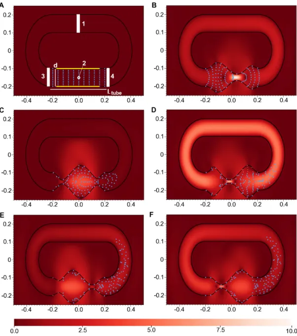
Figure 1.Panels showing racetrack circulatory system and compression region with speed across the simulation area (background color) and light-blue flow marker particles. A: Initial simulation conditions (t=0.0) showing racetrack circulatory system (black lines), tube diameterd(white vertical line), compression region,Ltube(white horizontal line between white boxes 3 and 4), tethered region (yellow
bars) and marker particles (light blue dots). Areas over which data were collected are labeled as white boxes and a white/black point (see text for details on calculations). B: Simulation att=0.4. C:
Simulation att=0.8. D: Simulation att=1.2. E: Simulation att=1.6. F: Simulation att=2.0. Color scale units non-dimensional speed.
P
re
P
rin
t0=f∗t,
whereL,U, and 1/f∗are characteristic flow length, velocity, and time scales respectively. In this paper, 112
we chooseLto be the diameter of the elastic section of the tube, f∗to be the beat frequency of our base 113
case, and the characteristic velocity asU=L f∗. Note theUdescribes the velocity in terms of heart tube 114
lengths per beat. 115
The dimensionless bending stiffness of the boundary may then be calculated as
k0bend= kbend
ρU2L3, (6)
wherekbend is the flexural stiffness of the boundary. The dimensionless spring stiffness may be written as
k0= k
ρU2L, (7)
wherekis the spring stiffness which describes the resistance to stretching. 116
The dimensionless pressure can then be defined as
p0= p
ρU2, (8)
wherepis the dimensional pressure andUis the characteristic velocity. 117
Of particular relevance to internal biological flows is the Womersley number (Wo). TheWodescribes to what extent unsteady effects matter in pulsatile flows. It is given by the following equation,
Wo=d
r
ω
ν, (9)
whereω is the frequency of the pulse,dis the diameter of the tube, andνis the kinematic viscosity of the
118
fluid. Within the context of a blood vessel, when the value ofWois high, the velocity profile is nearly 119
flat over most of the cross-section and there is a small region near the vessel wall known as the boundary 120
layer where viscous effects are important. Also, the flow at the center of the tube is inertial and pulsatile. 121
At the other low extreme end ofWo, the velocity profile over the vessel cross-section is parabolic, and the 122
flow is quasi-steady and viscous dominated. The transient effects can be ignored whenWois sufficiently 123
small, generally whenWo<1, and this is common in the case of microcirculation. Unless otherwise 124
noted, we vary theWoby changing the viscosity of the fluid only. 125
2.3 Numerical Method 126
We used an adaptive and parallelized version of the immersed boundary method, IBAMR (Griffith, 2014). 127
IBAMR is a C++ framework that provides discretization and solver infrastructure for partial differential 128
equations on block-structured locally refined Eulerian grids (Berger and Oliger, 1984; Berger and Colella, 129
1989) and on Lagrangian (structural) meshes. IBAMR also includes infrastructure for coupling Eulerian 130
and Lagrangian representations. 131
The Eulerian grid on which the Navier-Stokes equations were solved was locally refined near the 132
immersed boundaries and regions of vorticity with a threshold of|ω|>0.1. This Cartesian grid was 133
organized as a hierarchy of four nested grid levels, and the finest grid was assigned a spatial step size of 134
dx=D/512, whereDis the length of the domain. The ratio of the spatial step size on each grid relative 135
to the next coarsest grid was 1:4. The numerical parameters used for the simulations are given in Table 1. 136
2.4 Model of Peristalsis 137
A numerical model of an elastic heart tube connected to a rigid racetrack was constructed to study high 138
amplitude peristaltic flows. The racetrack design was used for easy comparison to previous models of 139
tubular heart pumping (e.g.Jung and Peskin, 2000; Hickerson et al, 2005b; Baird et al, 2014; Avrahami 140
and Gharib, 2008; Lee et al, 2012). The racetrack section was constructed by connecting two sections of 141
straight tube (one of which represents the elastic heart) to curved sections. The resting diameter of the 142
racetrack was constant throughout its length. Dimensions and elastic properties of the racetrack are given 143
in Table 2, and the model set up is shown in Fig. 1A. 144
P
re
P
rin
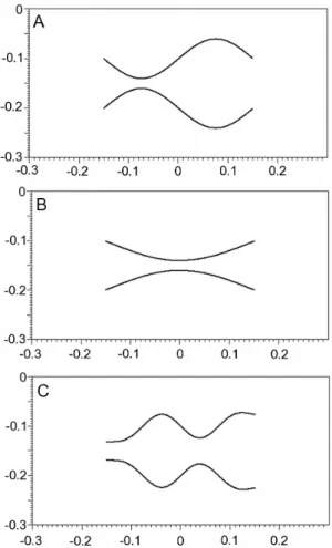
Figure 2.Panels showing no-racetrack design and several waveforms at simulation time = 2 seconds. Waveforms are the result of keeping a constant speed of compression wave,c=3.0, while altering the frequency of compression wave, f. A: f=1.0 (default value), B: f=0.5, C: f=2.0. Note that the domains in this figure have been reduce to show detail of the waveforms and do not reflect the domain on which the simulations were performed.
Table 1.Parameter values for two-dimensional immersed-boundary simulations.
Parameter value
Maximum time step (dt) 0.00001 Minimum Eulerian spatial step (dx) 0.01952 Lagrangian spatial step (ds) 0.00976
Domain size (D) 10.0
Refinement ratio (Rf) 4:1
P
re
P
rin
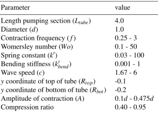
Table 2.Dimensionless parameter values for the peristalsis model.
Parameter value
Length pumping section (Ltube) 4.0
Diameter (d) 1.0
Contraction frequency (f) 0.25 - 3 Womersley number (Wo) 0.1 - 50 Spring constant (k0) 0.03 - 100 Bending stiffness (k0bend) 0.001 - 1
Wave speed (c) 1.67 - 6
ycoordinate of top of tube (Rtop) -0.1 ycoordinate of bottom of tube (Rbot) -0.2
Amplitude of contraction (A) 0.1d- 0.475d
Compression ratio 0.40 - 0.95
The bottom portion of the racetrack consisted of an elastic section of dimensionless lengthL=4.0 and dimensionless diameterd=1.0. The middle 3/4 of the tube was tethered to target points that drove the peristaltic motion. Note that the tube was initialized at rest in a straight configuration. The amplitude of the peristaltic wave increased from zero to its maximum amplitude after one pulse. To ensure conservation of volume inside the racetrack during pumping, the ends of the elastic section were allowed to deform as a result of the coupling between the elastic boundary and the fluid. Note that the sides and top of the racetrack were also tethered to target points that did not move. The target point stiffness,ktargwas set
equal to the spring stiffnessk. This parameter can be adjusted to minimize the distance between the actual boundary point and its target position. The position of the target points was determined by the following equation,
ytop,bot=Rtop,bot±Asin(2πf t+2πcxt) (10)
whereytop,botis they-coordinate of the top or bottom of the tube,Rtop,botis the distance of the top or
145
bottom of the tube from the horizontal centerline of the racetrack,Ais the amplitude of the contraction, f 146
is the frequency of contraction,cis the wave speed, andxtis the horizontal distance from the beginning
147
of the prescribed motion. The compression ratio gives the percent occlusion, and is equal to 2A. 148
In addition to the racetrack design, we constructed an open model of peristalsis which consisted of 149
only the elastic heart tube on the same domain (Fig. 2). The heart tube was driven in an identical way to 150
the racetrack design. This design allowed us to eliminate the possibility of Liebau pumping in our closed, 151
racetrack model by removing the flexible regions of heart tube that connected the contracting region to 152
the rigid racetrack. 153
2.5 Parameter Sweeps 154
We varied the values of four parameters in five separate sets of simulations. 1)Wowas changed by altering 155
the dynamic viscosityµof the fluid within the tube, which altersνin Equation 9 sinceν=µ/ρ, where
156
ρis fluid density.Woranged from 0.1 to 10. 2) Tube occlusion was changed by altering the amplitude of
157
contractionAin Equation 10 by some factor (compression ratio), which ranged from 40% tube occlusion 158
(compression ratio = 0.4) to nearly complete occlusion of the tube (compression ratio = 0.95). 3) The 159
speed of compression wave 4) the frequency of compressions (f in Equation 10) was changed, ranging 160
from 0.5 to 2.0, while allowing the speed of compression wave,c, to increase linearly. 5) The frequency 161
of compressions (f in Equation 10) was changed while holding the speed of the compression wave,c, 162
constant. Note that the no-racetrack design was used only for sweeps of compression wave frequency. 163
The default parameter values used for simulation sweeps other than the parameter of interest are: 164
Wo=1, f∗=1,c=3.0, and compression ratio=0.8. 165
2.6 Data Analysis 166
For each simulation, several calculations were made on fluid flow velocity in VisIt 2.5.2 (Childs et al, 167
2012) (for the racetrack design), Matlab (for the no-racetrack design), andR(Team, 2011) (both designs). 168
The compression wave propagated along the compression tube from left to right which drove fluid flow in 169
P
re
P
rin
the counter-clockwise direction around the racetrack (Fig. 1A-F). As a result, all positive flow speeds 170
indicate counter-clockwise flow (in the direction of the propagating compression wave) and negative 171
values indicate clockwise flow (opposite to the direction of the propagating compression wave). 172
Uavg: At each time point in the simulation, the non-dimensional magnitude of velocity|u0|of fluid
173
flow was spatially averaged across the cross-section of the upper tube of the racetrack indicated by a white 174
box labeled 1 in Fig. 1A. These mean speeds were then temporally averaged over the entire simulation to 175
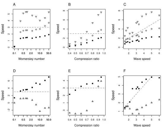
find the average speed per simulationUavg, presented in Fig. 5A-C (black circles) and Fig. 8A (black and
176
gray circles). 177
Umax,t, Umax: The non-dimensional maximum magnitude of velocity across the same section of
178
tube (white box labeled 1 in Fig. 1A) was also calculated for each time point of the simulation,Umax,t.
179
Fig. 3 showsUmax,tversus dimensionless time. These numbers were temporally averaged over the entire
180
simulation to find the average maximum speed per simulation,Umax, presented in Fig. 5A-C (white
181
diamonds) and Fig. 8A (white and gray diamonds). 182
Upeak: Using the non-dimensional, maximum speeds across the upper section of tube (white box
183
labeled 1 in Fig. 1A) for each simulation time step, peak speeds (maximum of maximum speed) were 184
found for each pulse. For each simulation, the peak speeds over each pulse were averaged to find the 185
average peak speed for each simulation,Upeak.
186
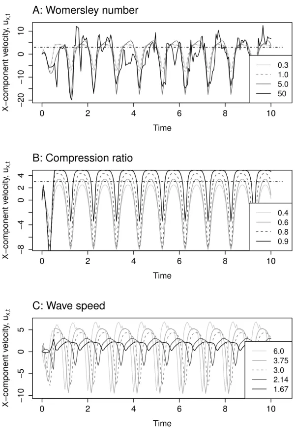
um, ux,t, ux: To characterize some of the dynamics in the compression region, the instantaneous,
187
non-dimensional magnitude of velocity (|u0|, speed) andx-component of fluid flow velocity,ux,t, were
188
sampled at each time at one point in the center of the compression tube, indicated by the white/black 189
dot labeled 2 in Fig. 1A. For thex-component of velocity, the instantaneous component of velocity for 190
each time stepux,tversust0are presented in Fig. 4. These speeds were then temporally averaged across
191
the entire simulation to find the average speed or magnitude of velocity (um) and averagex-component
192
of velocity (ux) for each simulation. These speeds are presented in Fig. 5D-F as black squares (um) and
193
triangles (ux) and in Fig. 8B as black and gray squares (um) and black and gray triangles (ux).
194
pin, pout,∆p: Non-dimensional pressure,p0, at each time step in the simulation was spatially averaged
195
across two cross-sections of the racetrack near the compression region: the inflow region (Fig. 1A, white 196
box 3) and outflow region (Fig. 1A, white box 4). The inflow pressures were subtracted from the outflow 197
pressures to find the pressure difference at each time step and averaged across the entire simulation to find 198
the average inflow pressurepin, the average outflow pressurepout, and average pressure difference (∆p)
199
for each simulation. These pressures are presented in Fig. 7A-D as connected circles (pin), connected
200
diamonds (pout) and dotted triangles (∆p).
201
For the no-racetrack design, the average volume flow ratevavgwas calculated using Matlab. The
202
averagex-component of velocity across the opening of the heart tube was calculated and then divided 203
by the diameter of the opening at that time point. These values were then temporally averaged across 204
simulation time to findvavg.
205
3 RESULTS
206Results discussed below are for the racetrack design unless otherwise noted. 207
3.1 Womersley number 208
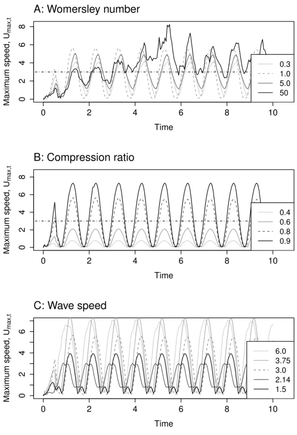
Flow speeds in the racetrack.Umax,t is graphed against simulation time for severalWoin Fig. 3A. Note
209
that theWowas varied by changing the viscosity of the fluid rather than the pulse frequency and/or the 210
wave speed. The dashed line shows the constant wave speed for these simulations. Fluid flow speeds 211
exhibit pulsatile behavior forWoof 5 and below. Unsteady behavior is observed forWo=50, likely due 212
to inertial effects and the formation of strong vortices in the tube. In all cases, the maximum dimensionless 213
flow speed is greater than the wave speed for part of the cycle. 214
215
Uavg,Umax, andUpeakare graphed against Womersley number (Wo) in Fig. 5A. Non-linear
relation-216
ships exist between each of the dimensionless flow speed metrics andWo, where theWowas varied by 217
changing the viscosity.Uavgtend to steadily increase with increasingWo, while average peak flow speeds
218
are greatest aroundWo=1 and 50.Upeakare greater than the speed of the compression wave,c, for all 219
Woand show variability with simulation time for values ofWo>10 (Fig. 3A). 220
221
P
re
P
rin
0
2
4
6
8
10
0
2
4
6
8
Time
Maxim
um speed, U
max,t
0.3 1.0 5.0 50
A: Womersley number
0
2
4
6
8
10
0
2
4
6
8
Time
Maxim
um speed, U
max,t
0.4 0.6 0.8 0.9
B: Compression ratio
0
2
4
6
8
10
0
2
4
6
Time
Maxim
um speed, U
max,t
6.0 3.75 3.0 2.14 1.5
C: Wave speed
Figure 3.Umax,tvs. simulation timet0. Dotted lines indicate default values for each parameter. Positive
speed indicates movement of fluid in the counter-clockwise direction around the racetrack. Horizontal dot-dash line indicates the non-dimensional speed of the compression wave for A and B. A: Womersley number, B: compression ratio, C: non-dimensional speed of the compression wave,c.
P
re
P
rin
0
2
4
6
8
10
−20
−10
0
10
Time
X−component v
elocity
, u
x,t
0.3 1.0 5.0 50
A: Womersley number
0
2
4
6
8
10
−8
−4
0
2
4
Time
X−component v
elocity
, u
x,t
0.4 0.6 0.8 0.9
B: Compression ratio
0
2
4
6
8
10
−10
−5
0
5
Time
X−component v
elocity
, u
x,t
6.0 3.75 3.0 2.14 1.67
C: Wave speed
Figure 4.ux,tvs. dimensionless time,t0, for a point at the center of the compression tube. Positive speed
indicates movement of fluid in the counter-clockwise direction around the racetrack. Dotted lines indicate default values for each parameter. Horizontal dotted-dashed line indicates the non-dimensional speed of the compression wave,c, for A and B. A: Womersley number, B: compression ratio, C: non-dimensional compression wave speed,c.
P
re
P
rin
0.1 0.5 2.0 10.0 50.0
0
1
2
3
4
5
Womersley number
Speed
0.1 0.5 2.0 10.0 50.0
A
0.4 0.5 0.6 0.7 0.8 0.9 1.0
0
2
4
6
8
Compression ratio
Speed
B
2 3 4 5 6
0
2
4
6
8
Wave speed
Speed
C
0.1 0.5 2.0 10.0 50.0
−2
0
2
4
6
Womersley number
Speed
0.1 0.5 2.0 10.0 50.0
D
0.4 0.5 0.6 0.7 0.8 0.9 1.0
0
1
2
3
4
Compression ratio
Speed
E
2 3 4 5 6
1
2
3
4
5
Wave speed
Speed
F
Figure 5.A-C: Non-dimensional fluid speeds within the racetrack versus parameter forUavg(black
circles),Umax(white diamonds), andUpeak(white, inverted triangles) across a section of tube (see text for
details of calculations). Positive speed indicates movement of fluid in the counter-clockwise direction around the racetrack. D-F:um(black squares) andux(white triangles) vs. parameter for a point at the
center of the compression tube. Non-dimensional compression wave speed,c, is noted on each plot as a dotted-dashed line. A,D: Womersley number, B,E: compression ratio, C,F: non-dimensional speed of the compression wave,c.
Flow speeds within the compression tube.umanduxare plotted againstWoin Fig. 5D.ux,t is plotted
222
against time for several simulations in Fig. 4A. The flow reversals (indicated by a change in sign) show 223
a non-parabolic flow profile in the pumping section forWo≥10. Whileum at this point increases
224
with increasingWo, the temporally averaged value ofuxdecreases and becomes negative forWo>1.
225
This indicates that flow is moving on average in clockwise direction, or opposite the direction of the 226
propagating compression wave. This phenomenon is due to significant back flow that occurs when the 227
tube rapidly expands behind the compression wave. 228
229
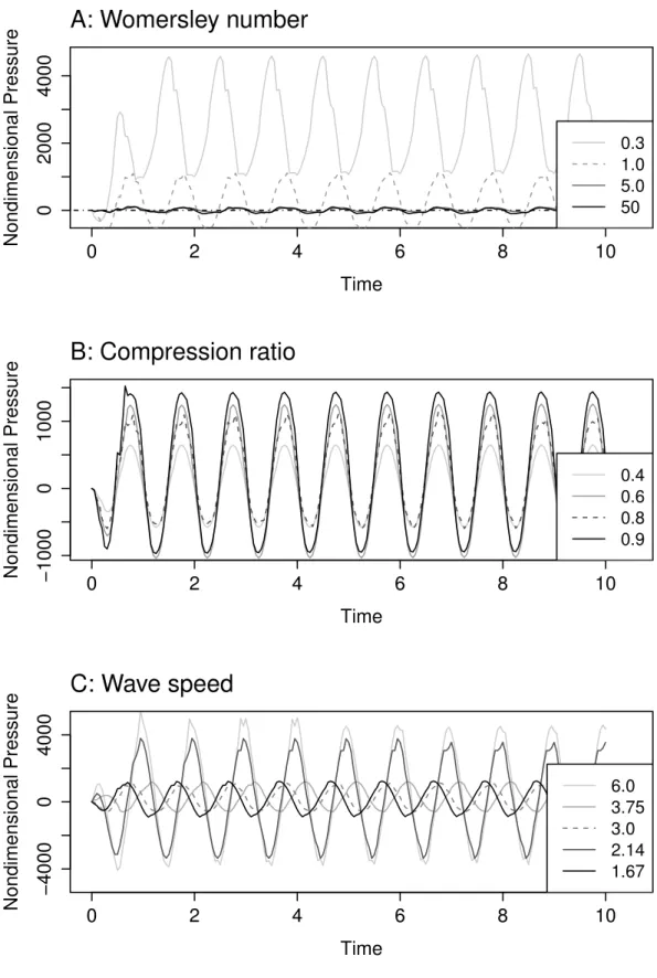
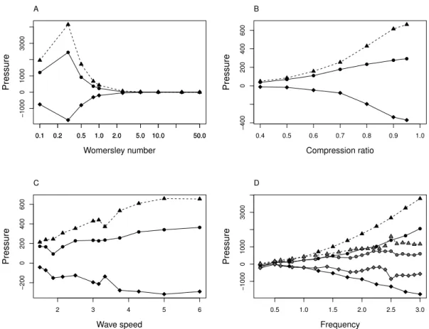
Pressure.For valuesWo<2, there are large differences in pressure (∆p). SinceWois varied by changing
230
viscosity, theWo<1 cases are viscous dominated, and this results in a high resistance of the fluid to 231
move through the tube.∆pare greatest atWo=0.3, with p0>4000 (Fig. 7A). Of note is the case where 232
Wo=0.1 and the pressure difference decreases relative toWo=0.3. Note in Fig. 5A that the flow speed 233
at thisWodrops to almost zero. For a compression ratio of 0.8, the peristaltic pump is not able to drive 234
highly viscous flow around the racetrack, and the pressure difference between the inflow and outflow tracts 235
drops. For valuesW ≥2, pressure differences between the two regions approach zero as the resistance to 236
flow decreases with decreasing viscosity. Non-dimensional pressurep0is reported versus time in Fig. 6A 237
for varying values ofWo. 238
3.2 Tube Occlusion 239
Flow speeds in the racetrack.Umax,t is graphed against dimensionless time for several compression
240
ratios in Fig. 3B. Note thatUmax,t does not exceedcfor compression ratios set to 0.6 and less. For
241
P
re
P
rin
0
2
4
6
8
10
0
2000
4000
Time
Nondimensional Pressure
0.3 1.0 5.0 50
A: Womersley number
0
2
4
6
8
10
−1000
0
1000
Time
Nondimensional Pressure
0.4 0.6 0.8 0.9
B: Compression ratio
0
2
4
6
8
10
−4000
0
4000
Time
Nondimensional Pressure
6.0 3.75 3.0 2.14 1.67
C: Wave speed
Figure 6. p0vs. dimensionless time,t0, for a point at the center of the compression tube. Dotted lines indicate default values for each parameter. Horizontal dotted-dashed line indicates the non-dimensional speed of the compression wave,c, for A and B. A: Womersley number, B: compression ratio, C: non-dimensional compression wave speed,c.
P
re
P
rin
large compression ratios of 0.8-0.9,Umax,treaches speeds of nearly double the value ofc. In all cases
242
considered,Umax,t is positive, and the flow moves in the counterclockwise direction at the top of the
243
racetrack. 244
245
Uavg,Umax, andUpeakare graphed against compression ratio in Fig. 5B. Each metric of the flow speed
246
has a non-linear, increasing relationship with increasing compression ratios. For compression ratios 247
under 0.7, corresponding to 70% tube occlusion,Upeak does not exceedcwhich is consistent with a
248
low-amplitude approximation of peristalsis (Fig. 3B). However, for values 0.7 and above, the average 249
peak flow speeds exceedc. 250
251
Flow speeds within the compression tube. Fig. 4B reportsux,t measured at the center of the
com-252
pression region as a function of dimensionless time for different compression ratios. Note that in all 253
cases, significant backflow occurs as the tube rapidly expands behind the compression wave. Backflow 254
is minimized at the highest compression ration of 0.9. Fig. 5E reports the temporally averaged speeds, 255
umandux, versus compression ratio. Higher compression ratios lead to higher forward flow speeds, as
256
evidenced by the increase inux relative to overall magnitude in Fig. 5B.ux exceeds the speed of the
257
compression wave for the highest values (≥0.9).umstarts to exceedcas low as compression ratio = 0.6
258
(Fig. 4B). 259
260
Pressure.Pressure differences between the inflow region (Fig. 1A at 3) and outflow region (Fig. 1A at 4)
261
are small for lower compression ratios and grow non-linearly with increasing tube occlusion (Fig. 7B). 262
The higher pressure differences correspond to the larger flow speeds generated by the higher compression 263
ratios. Non-dimensional pressurep0is reported versus time in Fig. 6B for varying values of compression 264
ratio. 265
3.3 Speed of Compression Wave,c 266
Flow speeds in the racetrack.In this set of simulations, the pulsing frequency is held constant andc
267
is varied. Umax,t is graphed against dimensionless time for several wave speeds in Fig. 3C. Note that
268
changingcwhile holding the frequency constant has the effect of changing the wave form (see Fig. 2). 269
The base case wave speed,c=3.0 was halved and doubled. As expected, lower values ofcresulted in 270
slow flows and higher values ofcresulted in faster flows. 271
272
Fig. 5C presentsUavg,Umax, andUpeakversuscfor the upper section of the racetrack. All three speeds
273
have a non-linear and increasing relationship with increasing wave speed, with average peak speeds being 274
consistently higher thanc. There is a small dip in fluid speeds around valuec=3.33 which is consistent 275
across all three measures of fluid speed. 276
277
Flow speeds within the compression tube.Fig. 4C reportsux,tas a function of dimensionless time for
278
different wave speeds. Note that there is significant backflow for the higher wave speed cases. In Fig. 5F, 279
the temporally averaged speedsumanduxmeasured at a point within the compression tube are plotted
280
against the wave speed. All three speed metrics have a similar non-linear relationship withc. Speeds 281
increase overall with increasingc. 282
283
Pressure.Pressures across both the inflow region (Fig. 1A at 3) and outflow region (Fig. 1A at 4) shares
284
a non-linear relationship withc, similar to the relationship seen between fluid flow speed and wave speed 285
(Fig. 7C). Generally, increasing wave speed also increases the pressure difference between the two points. 286
Note that the pressure difference dips aroundc=3.33, just asUavg,Umax, andUpeakalso drop at this
287
value ofc. Non-dimensional pressurep0is reported versus time in Fig. 6C for varying values ofc. 288
3.4 Compression Wave Frequency 289
Here we consider the following two cases: 1) frequency and wave speed are varied proportionally such 290
that the waveform along the compression tube is unchanged, and 2) frequency is varied while the wave 291
speed is held constant. This allows us to consider the cases when wave speed is coupled to and decoupled 292
from changes in the pulse frequency. 293
P
re
P
rin
0.1 0.2 0.5 1.0 2.0 5.0 10.0 50.0
−1000
0
1000
3000
Womersley number
Pressure
0.1 0.2 0.5 1.0 2.0 5.0 10.0 50.0
A
0.4 0.5 0.6 0.7 0.8 0.9 1.0
−400
0
200
400
600
Compression ratio
Pressure
B
2 3 4 5 6
−200
0
200
400
600
Wave speed
Pressure
C
0.5 1.0 1.5 2.0 2.5 3.0
−1000
0
1000
3000
Frequency
Pressure
D
Figure 7.Pressure versus parameter across two sections of the racetrack. pin: circles, solid line;pout:
black diamonds, solid line;∆p: black triangles, dotted line. A: Womersley number, B: compression ratio, C: non-dimensional speed of the compression wave,c, and D: non-dimensional compression-wave frequency, f. For D, frequencies with constant wave speed are gray and frequencies with varying wave speeds are black.
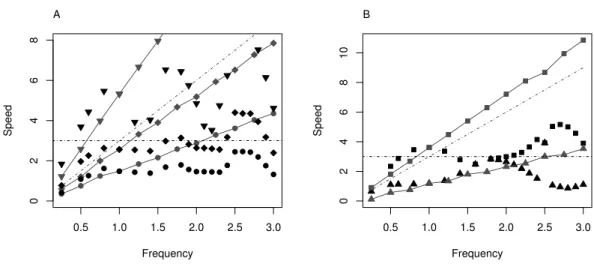
3.4.1 Variable Wave Speed 294
Flow Speed. Fig. 8A showsUavg,Umax, andUpeak as a function of the pulse frequency, f∗, for the
295
racetrack design. The grey data connected by lines shows the case when the compression wave speed is 296
allowed to change proportionally with f∗. In this case, all measures of speed show a linear relationships 297
with f∗. The dashed line shows the wave speed, andUmaxis close to the wave speed across all frequencies
298
considered.Upeakalso varies linearly with f∗and is higher than the wave speed. (Fig. 8B) showsum
299
anduxmeasured in the compression region as a function of f∗. The grey data shows the cases wherec
300
varies with f∗, and a clear linear relationship is observed. The linear relationships between flow speeds 301
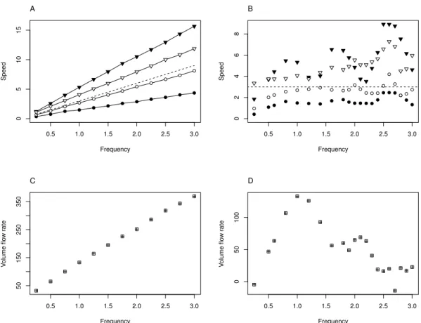
(UavgandUpeak) andf for flows generated in the no-racetrack model as well (Fig 9A). Additionally,Upeak
302
exceedcfor the no-racetrack design. 303
304
Volume Flow Rate.For the no-racetrack design, the volume flow rate,vavg, has a linear relationship with
305
compression frequency,f, whencincreases with increasing f (Fig. 9C). 306
307
Pressure.Fig. 7D shows the relationship between pressure,p0, and compression frequency,f, for cases
308
when the wave speed,c, changes proportionally with frequency (black items).p0inshows a nonlinear but 309
regular increase with increasing f, andpoutshows a nonlinear decrease with increasing frequency. The
310
pressure difference,∆pbetween the inflow and outflow tract increases in a regular and nonlinear way
311
with f. 312
P
re
P
rin
0.5 1.0 1.5 2.0 2.5 3.0
0
2
4
6
8
Frequency
Speed
A
0.5 1.0 1.5 2.0 2.5 3.0
0
2
4
6
8
10
Frequency
Speed
B
Figure 8.Non-dimensional fluid speed vs. non-dimensional compression wave frequency, f, for two cases: simulations with constant compression wave speed,c, (black items, no lines) or variablec(gray, solid line). Positive speed indicates movement of fluid in the counter-clockwise direction around the racetrack. A:Uavg(circles),Umax(diamonds), andUpeak(inverted triangles) measured in the upper tube
of the racetrack. (See text for description of calculations.) B:um(squares) andux(triangles) measured at
a point within the compression region of the tube.
3.4.2 Constant Wave Speed 313
Flow speeds in the racetrack. When compression wave speed is held constant while the pumping
314
frequency increases, all measures of fluid speed have markedly non-linear relationships with compression 315
frequency. Note that this has the effect of changing the wave form along the length of the compression 316
region. Within the upper section of the racetrack,Uavg,Umax, andUpeakshow an increasing, oscillatory
317
pattern with distinct peaks near f =0.8,1.6,and 2.5 (Fig. 8A). This pattern is more pronounced for 318
theUpeak.Upeakgreatly exceed the compression wave speed,c.Upeakis triple the wave speed nearf=2.5.
319
320
Flow speeds within the compression tube for the racetrack design.umanduxalso share a non-linear
321
relationship with the contraction frequency, f. This graph is characterized by oscillations, but peak flow 322
speeds within the compression tube do not correspond to the pattern seen within the racetrack (Fig. 8B). 323
324
Flow speeds for the no-racetrack design.UavgandUpeakshow a similar non-linear relationship with f
325
whencis held constant (the racetrack and no-racetrack designs are compared in Fig. 9B). Peaks in both 326
speeds are seen around f =0.8,1.6, and 2.5. Values ofUpeakare consistently abovec.
327
328
Volume Flow Rate.For the no-racetrack design, the volume flow rate,vavg, has a non-linear relationship
329
with compression frequency, f, whencis held at 3.0 (Fig. 9D). 330
331
Pressure. Fig. 7D shows the relationship between pressures, p0in,p0out and∆p, and frequency, f, for
332
constant wave speed (gray items). Pressures show a non-linear relationship with frequency, as in the case 333
of fluid flow speed. 334
4 DISCUSSION
3354.1 Evaluating large-amplitude, short-wave peristaltic pumps against the technical defi-336
nition of peristalsis 337
M¨anner et al (2010) summarizes 6 qualities of technical peristaltic pumps often used to evaluate biological 338
pumps based on small-amplitude and/or long-wave approximation of peristalsis. Our direct, numerical 339
simulation of peristalsis adheres to a simpler, more inclusive definition of peristalsis: having a non-340
stationary compression wave that travels uni-directionally down a tube with no structurally fixed direction 341
P
re
P
rin
0.5 1.0 1.5 2.0 2.5 3.0
0
5
10
15
Frequency
Speed
A
0.5 1.0 1.5 2.0 2.5 3.0
0
2
4
6
8
Frequency
Speed
B
0.5 1.0 1.5 2.0 2.5 3.0
50
150
250
350
Frequency
V
olume flo
w r
ate
C
0.5 1.0 1.5 2.0 2.5 3.0
0
50
100
Frequency
V
olume flo
w r
ate
D
Figure 9.Top row: Non-dimensional fluid speed vs. non-dimensional compression wave frequency, f, for two cases: with a connected racetrack (black items) and with no circulatory system or rigid ends (white items). Positive speed indicates movement of fluid in the counter-clockwise direction around the racetrack.Uavg(circles) andUpeak(inverted triangles) measured in the upper tube of the racetrack
(racetrack) and the mouth of the contracting region (no racetrack). Dotted lines report the speed of the compression wave,c. A. Simulations with variablec. B. Simulations with constantc. Bottom row: Volume flow rate,vavg, versus compression-wave frequency, f, for C. simulations with with variablec,
and D. simulations with constantc.
of flow. The geometry considered in this paper violates the long-wave approximation (the full wavelength 342
is 4 times the diameter for the base case) and the small-amplitude approximation (compressions up to 343
95% are considered). Furthermore, theWowas varied from 0.1 to 50, spanning cases where both inertia 344
and viscosity are significant. Note that this model was not developed to capture the specific dynamics of 345
any particular tubular heart but rather to consider highly nonlinear dynamics. 346
Our models incorporates the most basic features of peristalsis and produces flow characteristics that 347
run counter to those listed in the technical definition. Our model generates pulsatile fluid flow forWoof 5 348
and less at high compression ratios (Fig. 3A and B); flow speeds that show non-linear relationships when 349
either the compression wave speed or the pulsing frequency is fixed (Fig. 5C); and peak flow speeds that 350
exceed compression wave speeds in most cases (Figs. 3A-C, 5A-C, and 9A-B). These results are similar 351
to the results of other valveless, peristaltic models with cardiac cushions (Taber et al, 2007). When flow 352
speeds are measured in the compression section, significant back flow can be observed. 353
Additionally, the model shows that flow speeds can have either a linear or non-linear relationship 354
with compression frequency, depending on how the speed of the compression wave is handled. A linear 355
relationship between flow speed and compression frequency results when the speed of the compression 356
wave increases linearly with compression frequency (Figs. 8A and 9A,C), demonstrating that flow is 357
being driven by peristalsis and not another pumping mechanism. In this case, the wave form along the 358
P
re
P
rin
tube is the same, and the pump just operates faster. This is a feature of most mechanical pumps that does 359
not necessarily translate to biological pumps. In the case of a constant wave speed, the relationship is 360
strikingly non-linear between fluid speed and compression frequency (Fig. 8A and 9B,D). For these cases, 361
the wave form along the compression region changes (demonstrated in Fig. 2). This scenario corresponds 362
to situations when the pacemaker activity is altered while the propagation speed of an action potential is 363
constant. 364
4.2 Implications of large-amplitude, short-wave peristaltic pumps in biological fluid trans-365
port systems 366
Since many of the principles of the technical definition derived from mechanical pumps are violated by 367
our simple model, we suggest that the technical definition of peristalsis is inappropriate for evaluating the 368
pumping mechanism of biological pumps. While the definition appropriately describes some peristaltic 369
pumps, many biological pumps may fail simply because they violate the low-amplitude, long-wave 370
approximation used to establish the criteria in the technical definition. Simply decoupling compression 371
wave speed and frequency can also cause a pump to violate the technical definition even though it retains 372
the essential features of peristalsis (traveling wave of compression and no structurally fixed flow direction) 373
that mathematicians and biologists use. 374
There are many biological pumps that fail criteria in the technical definition of peristalsis but fit the 375
more inclusive definition. In tunicate hearts, heart beat frequency increases with increasing ambient 376
temperature but the conduction velocity that passes down the heart tube remains constant (Kriebal, 1967). 377
In mosquito hearts, hemolymph flow is not continuous and flow speed is greater than compression wave 378
speed (Glenn et al, 2010). For many tubular pumps, the contraction wave may nearly or even completely 379
occlude the tube. Other tubular pumps, such as the embryonic hearts of tunicates, are not much longer 380
than they are wide. Tubes with diameters on the order of their length violate the long-wave assumption. 381
4.3 Significance of the pumping mechanism to the embryonic heart 382
In the past 8 years, both peristalsis and dynamic suction pumping have been proposed as the mechanism 383
by which the early embryonic heart tube drives the flow of blood. The important point of this difference 384
for the case of understanding the evolution and development of the heart is the distinction between which 385
regions of the heart actively contract. If tubular hearts pump using dynamic suction pumping, then only 386
one region of the heart actively contracts, and the waves observed are passive and elastic. On the other 387
hand, if the pumping mechanism is peristalsis, then the heart actively contracts along its entire length. 388
This distinction has consequences for how the cardiac conduction system and the musculature develops. 389
In Forouhar et al (2006), work on embryonic zebrafish hearts, they present observations that demon-390
strate this valveless, tubular heart violates the technical definition of peristalsis. As we’ve shown with 391
this simple model of flow being driven by peristalsis, fluid flow can mimic each observation made on the 392
embryonic heart, including pulsatile flow both within the compressing tube (Fig. 4A-C) and far away from 393
the compression tube (Fig. 3A-C); peak flow speeds that exceed compression wave speeds (Fig. 5A-F and 394
9A-B); and a non-linear relationship between fluid flow and compression frequency that is very similar to 395
the relationship observed in their study (Fig. 8A and 9B). The results of our study suggest that peristalsis 396
cannot be ruled out as the pumping mechanism of the vertebrate embryonic heart, and that the exact 397
pumping mechanism requires further study since both mechanisms can result in similar features for cases 398
with nearly complete occlusion and diameter to length ratios on the order of 1:4. 399
The only observation that supports rejection of peristalsis as the pumping mechanism for the zebrafish 400
heart is that no active contraction down the length of tube was observed (Forouhar et al, 2006). However, 401
this observation has been disputed by others (M¨anner et al, 2010; Maes et al, 2011; Goenezen et al, 2012) 402
and was not supported by direct measurement of muscle activation or morphological features that would 403
suggest electrical activation of cardiac muscle was limited to one area of the heart. Many studies show 404
that the architecture required to propagate such a signal are present early during heart development and 405
that conduction throughout the myocardium is itself a critical component of normal cardiogenesis (Paff, 406
1938; Paff et al, 1964; Rottbauer et al, 2001; Chi et al, 2010). 407
5 ACKNOWLEDGEMENTS
408The authors would like to thank Boyce Griffith for his assistance with the use of IBAMR and to William 409
Kier for his thoughtful advice on this project over the years. This work was funded by a NSF DMS 410
P
re
P
rin
CAREER # 1151478 (to L. Miller) and by a NSF DMS Research and Training Grant # 5-54990-2311 (to 411
R. McLaughlin, R. Camassa, L. Miller, G. Forest, and P. Mucha). 412
REFERENCES
413Anderson M (1968) Electrophysiological studies on initiation and reversal of the heart beat inCiona 414
intestinalis. J Exp Biol 49:363–385 415
Aranda V, Cortez R, , Fauci L (2011) Stokesian peristaltic pumping in a three-dimensional tube with a 416
phase-shifted asymmetry. Physics of Fluids 23:081,901 417
Auerbach D, Moehring W, Moser M (2004) An analytic approach to the liebau problem of valveless 418
pumping. Cardiovascular Engineering: An International Journal 4(2):201–207 419
Avrahami I, Gharib M (2008) Computational studies of resonance wave pumping in compliant tubes. 420
Journal of Fluid Mechanics 608:139–160 421
Baird A, King T, Miller LA (2014) Numerical study of scaling effects in peristalsis and dynamic suction 422
pumping. Contemporary Mathematics 628:129–148 423
Berger MJ, Colella P (1989) Local adaptive mesh refinement for shock hydrodynamics. J Comput Phys 424
82(1):64–84 425
Berger MJ, Oliger J (1984) Adaptive mesh refinement for hyperbolic partial-differential equations. 426
J Comput Phys 53(3):484–512 427
Bringley T, Childress S, Vandenberghe N, Zhang J (2008) An experimental investigation and a simple 428
model of a valveless pump. Physics of Fluids 20:033,602 429
Ceniceros HD, Fisher JE (2012) Peristaltic pumping of a viscoelastic fluid at high occlusion ratios and 430
large weissenberg numbers. Journal of Non-Newtonian Fluid Mechanics 171-172(31-41) 431
Chi N, Bussen M, Brand-Arzamendi K, Ding C, Olgin J, Shaw R, Martin G, Stainier D (2010) Car-432
diac conduction is required to preserve cardiac chamber morphology. Proc Natl Acad Sci U S A 433
107(33):14,662–14,667 434
Childress S (2009) An Introduction to Theoretical Fluid Mechanics, Courant Lecture Notes, vol 19. 435
American Mathematical Society 436
Childs H, Brugger E, Whitlock B, Meredith J, Ahern S, Pugmire D, Biagas K, Miller M, Harrison C, 437
Weber GH, Krishnan H, Fogal T, Sanderson A, Garth C, Bethel EW, Camp D, R¨ubel O, Durant M, 438
Favre JM, Navr´atil P (2012) VisIt: An End-User Tool For Visualizing and Analyzing Very Large Data. 439
In: High Performance Visualization–Enabling Extreme-Scale Scientific Insight, pp 357–372 440
Christoffels VM, Moorman AFM (2009) Basic science for the clinical electrophysiologist. Circulation: 441
Arryhythmia and Electrophysiology 2:195–207 442
Davidson B (2007) Ciona intestinalis as a model for cardiac development. Semin Cell Dev Biol 18(1):16– 443
26 444
Forouhar AS, Liebling M, Hickerson A, Nasiraei-Moghaddam A, Tsai HJ, Hove JR, Fraser SE, Dickinson 445
ME, Gharib M (2006) The embryonic vertebrate heart tube is a dynamic suction pump. Science 446
312(5774):751–753 447
Fung YC, Yih CS (1968) Peristaltic transport. ASME E J Appl Mech 35:669–675 448
Gashev A (2002) Physiologic aspects of lymphatic contractile function. Annals of the New York Academy 449
of Sciences 979:178–187 450
Glenn J, King J, Hillyer J (2010) Structural mechanics of the mosquito heart and its function in bidirec-451
tional hemolymph transport. J Exp Biol 213:541–550 452
Goenezen S, Rennie M, Rugonyi S (2012) Biomechanics of early cardiac development. Biomech Model 453
Mechanobiol 11:1187–1204 454
Greenlee K, Socha J, Eubanks H, Thapa G, Pederson P, Lee W, Kirkton S (2013) Hypoxia-induced 455
compression in the tracheal system of the tobacco hornworm caterpillar,Manduca sextaL. J Exp Biol 456
216:2293–2301 457
Griffith B (2014) An adaptive and distributed-memory parallel implementation of the immersed boundary 458
(ib) method. URL https://github.com/IBAMR/IBAMR 459
Griffiths D, Constantinou C, Mortensen J, Djurhuus J (1987) Dynamics of the upper urinary tract: II. 460
the effect of variations of peristaltic frequency and bladder pressure on pyeloureteral pressure/flow 461
relations. Phys Med Biol 32(7):832–833 462
Hanin M (1968) The flow through a channel due to transversely oscillating walls. Israel J Tech 6:67–71 463
P
re
P
rin
Harrison J, Waters J, Cease A, Cease A, VandenBrooks J, Callier V, Klok C, Shaffer K, Socha J (2013a) 464
How locusts breathe. Physiology 28:18–27 465
Harrison JF, Waters JS, Cease AJ, VandenBrooks JM, Callier V, Klok CJ, Shaffer K, Socha JJ (2013b) 466
How locusts breathe. Physiology 28(1):18–27 467
Hickerson AI, Rinderknecht D, Gharib M (2005a) Experimental study of the behavior of a valveless 468
impedance pump. Experiments in fluids 38(4):534–540 469
Hickerson AI, Rinderknecht D, Gharib M (2005b) Experimental study of the behavior of a valveless 470
impedance pump. Experiments in Fluids 38(4):534–540 471
Jaffrin M, Shapiro A (1971) Peristaltic pumping. Annual Review of Fluid Mechanics 3:13–37 472
Jung E, Peskin CS (2000) Two-dimensional simulations of valveless pumping using the immersed 473
boundary method two-dimensional simulations of valveless pumping using the immersed boundary 474
method. SIAM J Sci Comput 23(1):19–45 475
Jung E, Lee S, Lee W (2008) Computational models of valveless pumping using the immersed boundary 476
method. Computer Methods in Applied Mechanics and Engineering 197:2329–2339 477
Kalk M (1970) The organization of a tunicate heart. Tissue and Cell 2:99–118 478
Krenn H (2010) Feeding mechanisms of adult Lepidoptera: structure, function, and evolution of the 479
mouthparts. Annu Rev Entomol 55:307–327 480
Kriebal M (1967) Conduction velocity and intracellular action potentials of the tunicate heart. J General 481
Physiology 50(8):2097–2107 482
Lee W, Socha J (2009) Direct visualization of hemolymph flow in the heart of a grasshopper (Schistocerca 483
americana. BMC Physiology 9(2):doi:10.1186/1472–6793–9–2 484
Lee W, Lim S, Jung E (2012) Dynamical motion driven by periodic forcing on an open elastic tube in 485
fluid. Commun Comput Phys 12:494–514 486
Liebau G (1954) ¨Uber ein ventilloses pumpprinzip. Naturwissenschaften 41:327–327, DOI 487
10.1007/BF00644490, URL http://dx.doi.org/10.1007/BF00644490 488
Liebau G (1955) Die stromungsprinzipien des herzens. Z Kreislaufforsch 44:677 489
Liebau G (1957) Die bedeutung der tragheitskrafte fur die dynamik des blutkreislaufs. Z Kreislaufforsch 490
46:428 491
Maes F, Chaudhry B, Ransbeeck PV, Verdonck P (2011) The pumping mechanism of embryonic hearts. 492
IFMBE Proceedings 37:470–473 493
M¨anner J, Wessel A, Yelbuz T (2010) How does the tubular embryonic heart work? looking for the physical 494
mechanism generating unidirectional blood flow in the valveless embryonic heart tube. Developmental 495
Dynamics 239:1035–1046 496
Paff G (1938) The beahvior of the embryonic heart in solutions of ouabain. Am J Physiol 122(3):753–758 497
Paff G, Boucek R, Klopfenstein H (1964) Experimental heart-block in the chick embryo. Anatomical 498
Record 149:217–223 499
Peskin CS (2002) The immersed boundary method. Acta Numer 11:479–517 500
Postma AV, Christoffels VM, Moorman AFM (2008) Developmental aspects of the electrophysiology of 501
the heart: Function follows form. Electrical Diseases of the Heart pp 24–36 502
Pozrikidis C (1987) A study of peristaltic flow. J Fluid Mech 180:515–527 503
Rottbauer W, Baker K, Wo Z, Mohideen M, Cantiello H, Fishman M (2001) Growth and function of the 504
embryonic heart depend upon the cardiac-specific L-type calcium channelα1 subunit. Developmental 505
Cell 1:265–275 506
Santhanakrishnan A, Miller LA (2011) Fluid dynamics of heart development. Cell Biochem Biophys 507
61(1):1–22 508
Shapiro A, Jaffrin M, Weinberg S (1969) Peristaltic pumpuing with long wave lengths at low reynolds 509
number. J Fluid Mech 37:799–825 510
Taber LA (2001) Biomechanics of cardiovascular development. Annu Rev Biomed 3:1–25 511
Taber LA, Zhang J, Perucchio R (2007) Computational model for the transition from peristaltic to pulsatile 512
flow in the embryonic heart tube. J Biomech Eng 129:441–449 513
Team RDC (2011) R: A Language and Environment for Statistical Computing. R Foundation for Statistical 514
Computing, Vienna, Austria, http://www.r-project.org/ edn 515
Teran J, Fauci L, Shelley M (2008) Peristaltic pumping and irreversibility of a stokesian viscoelastic fluid. 516
Physics of Fluids 20:073,101 517
Vogel S (2007) J Biosci 32(2):207–222 518
P
re
P
rin
Waldrop L, Miller LA (2015) The role of the pericardium in the valveless, tubular heart of the tunicate, 519
ciona savignyi, submitted. 520
Xavier-Neto J, Castro R, Sampaio A, Azambuja A, Castillo H, Cravo R, Simoes-Costa M (2007) Parallel 521
avenues in the evolution of hearts and pumping organs. Cell Mol Life Sci 64:719–734 522
Xavier-Neto J, Davidson B, Simoes-Costa M, Castillo H, Sampaio A, Azambuja A (2010) Heart Develop-523
ment and Regeneration, vol 1, 1st edn, Elsevier Science and Technology, London, chap Evolutionary 524
origins of the heart, pp 3–38 525