A DATA-DRIVEN APPROACH FOR OPERATIONAL IMPROVEMENT IN EMERGENCY DEPARTMENTS
Wanyi Chen
A dissertation submitted to the faculty of the University of North Carolina at Chapel Hill in partial fulfillment of the requirements for the degree of Doctor of Philosophy in the
Department of Statistics and Operations Research.
Chapel Hill 2018
Approved by: Nilay Argon Serhan Ziya Chuanshu Ji
c 2018 Wanyi Chen
ABSTRACT
WANYI CHEN: A Data-Driven Approach for Operational Improvement in Emergency Departments
(Under the direction of Nilay Argon and Serhan Ziya)
TABLE OF CONTENTS
LIST OF TABLES . . . 1
LIST OF FIGURES . . . 1
1 Introduction . . . 1
2 Dynamic Decision Making in a Queueing System with Secondary Service . . . 4
2.1 Introduction . . . 4
2.2 Literature Review . . . 7
2.3 Model Description . . . 9
2.4 Existence of a Stationary Optimal Policy . . . 13
2.5 Structure of the Optimal Policy . . . 15
2.6 Monotonicity of the Optimal Threshold . . . 18
3 Optimal Timing for Early Bed Request for Admitted Patients in an Emergency Department . . . 20
3.1 Introduction . . . 20
3.2 Literature Review . . . 22
3.3 The Fluid Model . . . 23
3.4 The Optimal Policy . . . 26
4 Numerical Study . . . 29
4.1 Introduction . . . 29
4.2 Heuristic Policies . . . 30
4.2.1 The Current System . . . 30
4.2.2 Fixed Threshold Policy (FT) . . . 30
4.2.3 Time-Dependent Threshold Policy (TT) . . . 31
4.2.5 Constrained Fixed Threshold Policy (CFT) . . . 33
4.3 Simulation Model . . . 38
4.3.1 Input Analysis . . . 40
4.3.2 Calibration and Validation . . . 43
4.4 Numerical Study . . . 45
4.5 Discussion . . . 48
5 Impact of Census on Emergency Department Providers’ Triage and Admission Decisions . . 49
5.1 Introduction . . . 49
5.2 Methods . . . 51
5.2.1 Study Design and Setting . . . 51
5.2.2 Data Analysis . . . 51
5.2.3 Statistical Modeling . . . 54
5.3 Results . . . 56
5.4 Discusssion . . . 61
5.5 Conclusion . . . 63
6 Conclusion . . . 64
A APPENDIX: PROOF OF THEOREMS, LEMMAS, AND SUPPLEMENTARY TABLES . 67 A.1 Proof of Lemma 1 . . . 67
A.2 Proof of Lemma 2 . . . 68
A.3 Proof of Lemma 3 . . . 71
A.4 Proof of Lemma 4 . . . 79
A.5 Proof of Theorem 4 . . . 81
A.6 Single-Server Clearing Model . . . 90
A.7 Tables for Chapter 5 . . . 92
LIST OF TABLES
4.1 Estimated for 9am to 5pm . . . 34
4.2 Estimated γ under different admission thresholds for 9am-5pm . . . 35
4.3 Estimated δ under different admission thresholds for Λ = 0.5 . . . 37
4.4 Estimated δ under different admission thresholds for Λ = 1 . . . 37
4.5 Estimated δ under different admission thresholds for Λ = 1.5 . . . 37
4.6 Estimated δ under different admission thresholds for Λ = 2 . . . 37
4.7 Ward hours and bed capacity . . . 39
4.8 Service time distributions for adult patients . . . 41
4.9 Service time distributions for pediatric patients . . . 42
4.10 Boarding time distributions for adult patients . . . 42
4.11 Boarding time distributions for pediatric patients . . . 43
4.12 Ward hours and bed capacity . . . 44
5.1 Breakdown of patient characteristics for variables of interest. . . 53
5.2 P-values from likelihood ratio tests for all independent variables included in the selected cumulative logit model for triage decisions and multivariate logistic regression model for disposition. . . 56
5.3 Odds ratios of Prob(high acuity) versus Prob(low or medium acuity) and Prob(medium or high acuity) versus Prob(low acuity), and corresponding 95% confidence intervals for intercept, census, race, gender, and age group. . . 57
5.4 Odds ratios of Prob(admit) versus Prob(discharge) and corresponding 95% confidence intervals for intercept, census, race, gender, acuity, age group, and pod. . . 58
A.1 Odds ratios of Prob(high acuity)/Prob(low or medium acuity) = Prob(medium or high acuity)/Prob(low acuity) for chief complaint (con-trast: other) from the model for the association between ED census and triage decisions. (A model where the two odds ratios were not necessarily the same for chief complaints provided similar results.) . . . 92
A.3 Odds ratios of Prob(admit) versus Prob(discharge) for interaction terms between ESI and age group (contrast: ESI3 and Age Group 18 to 40) from the model for the association between ED census and disposition decisions.
LIST OF FIGURES
3.1 Arrival rate (number of arrivals per hour) vs. hour-of-day based on UNC
ED 2012 data . . . 25
3.2 Service rate (number of patients served per hour) per server under normal operating conditions vs. hour-of-day based on UNC ED 2012 data . . . 25
4.1 Patient flow at The ED . . . 38
4.2 Sojourn Times Validation . . . 45
4.3 Length-of-stay (LOS) under CTT and FT . . . 47
4.4 Length-of-stay (LOS) under CTT and TT . . . 47
4.5 Length-of-stay (LOS) under CTT and CFT . . . 47
5.1 Marginal probabilities of different acuity levels versus census for a patient subgroup: Caucasian female, aged between 18 to 40, with abdominal pain. . . 61
CHAPTER 1 Introduction
Emergency departments (EDs) are gateways to hospitals and play a critical role in the US healthcare system. The majority of them are experiencing significant operational stress caused by overcrowding. Failure to serve on time can put patients at risk for suboptimal care and potential health harm. Researchers have been seeking to identify primary causes of ED overcrowding and ways to reduce its adverse effects to the extent possible (Olshaker, 2009), (Hoot and Aronsky, 2008), (Welch et al., 2011).
With this motivation, we formulated a queueing model in Chapter 2 that approximates the patient flow in the ED in a stylized fashion. Each job (patient) that arrives to the queueing system (i.e., the ED) belongs to one of two types. Type 1 jobs need only a primary service given by a single server while type 2 jobs need an additional secondary service. The primary service corresponds to the lump sum service patients receive at the ED and the secondary service refers to the inpatient admission procedure (the secondary service time corresponds to boarding). The type of a patient determines whether he/she will be admitted to the hospital. Secondary service is conducted by servers that are always available when it is initiated. However, primary server cannot serve a new job until secondary service of a job is over. Jobs incur waiting costs and there is an option of starting primary and secondary services at the same time with an extra cost. The decision is whether or not to use that option for each job given the probability that the job is of type 1. We formulate this problem as a Markov decision process and prove that the optimal policy that minimizes the long-run average cost is of threshold-type.
In Chapter 3, we take an alternative approach and build a deterministic and continuous fluid model aiming to capture the general behavior of patient flow in the ED. As mentioned earlier, when implementing early bed requests in the ED one needs to carefully manage the tradeoff between the cost of overcrowding associated with holding hospital admitted patients in the ED and the cost of wasting hospital resources by making too many early bed requests based on false admission prediction. Of course, knowing the relative magnitude of these two counteracting costs can aid in our decision making yet it might be unrealistic to estimate the cost of a false early bed request. Hence, in this alternative formulation, we impose a constraint on the length of time during which one can make early bed requests and thus speed up service. To be more specific, we treat the patients arriving to an ED as fluid flowing into a tank. The fluid is pumped out of the tank at some deterministic outflow rate as patients receive service at the ED. There is an option to speed up the outflow rate, which corresponds to the option of starting preparing the hospital bed for patients early on based on their predicted probability of admission to hospital. Using this fluid model we identify the optimal period of time during each day to use that option given the aforementioned operational constraint on the total amount of time early bed requests can be made.
consists of 12 months of all patient encounters at the UNC ED in 2012, we built a simulation model of the ED. We utilize this simulation model to evaluate the heuristics considered in terms of the improvement they bring in reducing patients’ length-of-stay, waiting, and boarding times.
CHAPTER 2
Dynamic Decision Making in a Queueing System with Secondary Service
2.1 Introduction
Mainly motivated by these novel practices, we consider a queueing system in which each arriving customer is either of type-1 or type-2. Customers of either type require primary service, which is provided by a single server (we will refer to this server as the server throughout the paper) while type-2 customers additionally require the secondary service. This secondary service is provided by another collection of servers, which are assumed to be infinitely many. All customers queue in front of the server. When the server picks up the next customer to serve, it cannot observe the type of the customer but can observe the probability that the customer is of type-2, i.e., that the customer will need the secondary service. Only after completion of the primary service, the server knows with complete certainty whether the customer will need the secondary service. However, there is nothing that prevents the primary and the secondary services to proceed simultaneously and thus the system controller can order the secondary service to start at the same time as the server starts the primary service even though the secondary service for that particular customer could be unnecessary.
If the controller does not initiate the secondary service together with the primary service, the server proceeds with the primary service and by the end of the service, it determines whether the customer needs the secondary service. If s/he does not (meaning a type-1 customer), the customer leaves right away and the server picks up the next customer. If the customer is of type-2, and thus needs the secondary service, the customer starts receiving the secondary service right away from the pool of infinitely many servers. However, the server cannot serve a new customer. It remains
blocked until the secondary service of the customer is over. If the controller initiates the secondary service together with the primary service, the server again proceeds with the primary service and it determines whether the customer needs the secondary service. If she does not or if she does but the secondary service, which started earlier together with the primary service, is already over, then the customer leaves right away and the server picks up the next customer. Each customer incurs a waiting cost, which is linearly increasing with the time s/he spends waiting. Without loss of generality, there is no cost associated with the primary service but the secondary service has a cost and this cost is smaller when it is started after the primary service is over.
more for the secondary service but is also taking a risk because the secondary service may in fact be completely unnecessary for that customer. Thus, the goal of the controller is to carefully manage this trade-off. More specifically, the objective of the controller is to minimize the long-run average cost the system incurs by identifying whether the secondary service should be initiated together with the primary service given the number of customers waiting and the probability that the customer who is about to start the primary service is of type-2.
The model broadly described above is stylized and is not meant to capture the motivating applications at a highly detailed, realistic level. Our goal in this paper is to provide some general insights and possibly pave the way for the analysis of more advanced formulations in the future. However, it might be necessary to provide some explanations for the reasons behind some of our modeling choices. It is likely clear to the reader that the customers in the model correspond to the patients arriving at the emergency department and the type of a customer determines whether the patient needs a diagnostic test in the first setting described above and whether the patient will eventually be admitted to the hospital in the second setting. Somewhat more difficult to see is what exactly the server corresponds to and what exactly it means to have an infinite collection of servers for the secondary service.
2.2 Literature Review
There are three streams of research relevant to the study undertaken in this paper, one con-cerned with the dynamic control of queues, and in particular the control imposed on the service pro-cess, one concerned with Business Process Management (BPM) and the evaluation of the changes in service structure along the dimension of cost, and the final one concerned with service outsourcing. With regard to dynamic control of queues via varying service rates, one commonality found in most literature, a similarity to our paper, is that the decision making is typically centered around the tradeoff between two kinds of costs, namely, the cost of holding customers in the queue, which is nondecreasing with respect to the queue length, and the cost of applying faster service rates, which is nondecreasing with respect to the service rates applied. Additionally, among the papers dealing with the characterization of optimal policies most of them show that they have certain monotonicity structure in terms of the queue lengths.
process with constant arrival rate and state-dependent service rates that can be chosen from a fixed subset. There is a nondecreasing cost-of-effort function on the subset of values that service rates can be chosen from and holding costs are continuously incurred as a nondecreasing function of the queue length. They find that the optimal service rates are nondecreasing as a function of queue length. They also present a method for computing the minimum achievable average cost.
As to the redesign of the underlying mechanics of business processes, Buzacott and John A. (Buzacott, 1996) gives a comprehensive review of different kinds of system structure reengineering and explores conditions under which such changes are beneficial. In general, a high degree of variability in task times seems to be necessary. In his paper, the scenario where several tasks are combined into one is a similar version of our problem in the sense that for both the purpose is to reduce or eliminate subdivision of the overall processing requirements into individual tasks, each performed by a different facility, person or machine. To be more specific, our model assumes there is the option of starting stage-2 service together with stage-1 service with a resulting service time of the maximum of the two. This is in parallel with the use of case teams, suggested by Hammer and Champy and summarized in the paper, where in our case the team corresponds to the team formed by stage-1 and stage-2 servers. Similar to their setting, each job is not complete until both tasks are complete and the next job cannot begin until the previous job is complete. The difference lies in the fact that with no collaboration, which in our case corresponds to starting stage-2 service after stage-1 service is complete, the next job cannot enter stage-1 service until both tasks on the previous job are complete. To our knowledge, most BPM research is primarily concentrated upon identifying the objective and developing heuristic policies for business processes through a qualitative perspective. Interested readers can refer to (Van Der Aalst, 2013) for a comprehensive review of the state-of-the-art in BPM research. On the other hand, this paper starts with a redesign of the service flow, namely, to conduct second stage service together with first stage service at the same time, and focuses on finding the dynamically optimal way to apply this control.
increase the holding cost. Hence the act of starting stage-2 service can be considered as outsourcing, and the decision-making is centered around balancing in-house holding cost and outsourcing cost (starting ahead is more expensive than starting on-demand). In relation to the literature on service outsourcing, our paper is most similar to (Ko¸ca˘ga et al., 2015). Most papers in this literature study contracting issues in the context of call center outsourcing, where a firm (which we will call the user) that sends some or all of its calls to an outside server (which we willl call the vendor) must determine appropriate terms for the contract to induce the vendor to make system-optimal decisions and the vendor must make decisions about staffing level and effort level. Unlike these papers, (Ko¸ca˘ga et al., 2015) focus on real-time routing decisions instead. They are faced with the issue of under/over-staffing in call centers when arrival rates are uncertain. To mitigate this issue, they find a joint policy for staffing and real-time call co-sourcing, i.e., by sometimes outsourcing calls, that minimizes long run average cost when there is staffing cost and costs associated with abandoments and outsourcing. They formulate a Markov decision process and propose a policy that uses a square-root safety staffing rule, and outsources calls in accordance with a threshold rule that is dependent on the queue length. They show that this policy is asymptotically optimal. Both the optimality of a threshold-type policy and the cost structure that influences dynamic decision making is very similar to our work presented here.
2.3 Model Description
complete. (In the rest of the paper, unless otherwise specified, “the server” will always refer to the server performing the primary service.) However, if primary service and secondary service are started simultaneously and primary service finishes first but it is revealed that secondary service is in fact not needed, the customer leaves right away and the server becomes immediately available for the next customer.
The system controller cannot observe the type of the customers before they go through primary service but it can observe the probability of any given customer being of type-2. The type of the customer is revealed with certainty only after the completion of primary service. Let Zk denote the random variable representing the probability that the kth customer to arrive to the system is of type-2. We assume that {Zk}∞k=1 is a sequence of independent and identically distributed (iid) random variables with the common discrete probability distribution specified asP{Zk =αi}=qi} for αi ∈Ω and k∈ {1,2, . . .}, where Ω ={α1, α2, . . . ,} is the set of possible values Zk can take. Without loss of generality, we assume thatαi is increasing ini. We also letα=P∞i=1qiαi so that
α represents the probability that a randomly chosen customer is of type-2.
let Ssz denote the same time if the services are performed in stage. Then,
Spz =
max(X1, X2) w.p. z
X1 w.p.1−z
,
and
Szs =
X1+X2 w.p. z
X1 w.p. 1−z
.
Thus, the benefit of choosing the parallel service option is that with probability z, the service time of the customer shortens to max(X1, X2) fromX1+X2. As we explain, next, however, there are costs associated with taking different actions and therefore choosing this option for all the customers may not be desirable.
Specifically, we assume that the system incurs a holding cost of Cw for each waiting customer per unit of time. The cost of performing secondary service after the completion of primary service is denoted by Cs and the cost of performing secondary service in parallel with primary service is denoted by Cp. Note that any cost of primary service is irrelevant and is thus ignored because all customers have to go through primary service. We assume throughout the paper that αiCs ≤Cp for all i, which implies that for any single customer in isolation the cost of performing parallel service is larger than the expected cost of performing service in sequence. An obvious sufficient condition for this assumption to hold is that Cs≤Cp, i.e., service in sequence does not cost more than service in parallel, which is likely to hold in our motivating applications where the cost under either service option would likely be about the same. The objective of the service controller is to minimize the long-run average cost for this system by determining when to choose parallel service and when to choose service in sequence depending on the system state.
and m = 3 corresponding to the state in which the server has already completed primary service and the customer is now going through secondary service. We restrict ourselves to the policy set Π, where any π ∈ Π is a stationary, non-idling, state-dependent policy, and is a mapping from the system stateX to the action space A={0,1} where 0 corresponds to the decision of starting a “service in sequence”, i.e., not initiating a secondary service together with primary service and 1 corresponds to the decision of starting a parallel service with the restriction that no action is available in state (0) and action 1 is only available in statesxwherex= (αi, n≥1), for somei, i.e. when there is at least one customer and either a primary or a secondary service has not already been completed for the customer because of a parallel service decision made earlier. Note that the policies we consider here can be seen as preemptive in the sense that the system controller can switch from “parallel service” to “service in sequence” at a decision epoch, which can correspond to either an arrival time or a service completion time, as long as neither primary nor secondary service is complete for the customer or from “service in sequence” to “parallel service” as long as the primary service of the customer is still in progress.
Using uniformization, the continuous-time MDP formulation can equivalently be written as a discrete-time MDP. Letβ=λ+γ1+γ2 denote the uniformization constant. We setβ = 1 without loss of generality. For anyx∈X,h(x) denotes the relative value or bias for statex. For expositional convenience below, we further define h(αj,0) =h(0) for j= 1,2, . . . as the relative value function although (αj,0) is not an element of the state spaceX. Finally, let g denote the long-run average cost under an optimal policy. Then, the optimality equations can be written as follows:
h(0) =λX
j
qjh(αj,1) + (γ1+γ2)h(0). (2.1)
For alln≥1, andαi ∈Ω,
h(αi, n) =nCw+λh(αi, n+ 1) + (1−αi)γ1 X
j
qjh(αj, n−1)
+αiγ1h(3, n) +γ2min{h(αi, n) +
αiγ1
γ2
Cs, h(2, n) +
γ1+γ2
γ2
whereh(αj,0) =h(0) =Pjqjh(αj,0), for allj. For all n≥1,
h(2, n) =nCw+λh(2, n+ 1) +γ1 X
j
qjh(αj, n−1) +γ2h(2, n), (2.3)
h(3, n) =nCw+λh(3, n+ 1) +γ2 X
j
qjh(αj, n−1) +γ1h(3, n). (2.4)
We know that if there is a solution to the optimality equations above, then there exists a stationary, deterministic policy, π∗ ∈ Π under which the long-run average cost is g = g∗ and the policy is described by the action that minimizes the right hand side of the optimality equation for each state x∈X.
2.4 Existence of a Stationary Optimal Policy
In this section, we show that under a particular condition on the arrival and service rates, the solution to the optimality equations exist and thus there exists an optimal stationary policy. The condition we need is that λγ1
1 + α γ2
<1. Recall that α is the probability that a randomly chosen customer is of type-2 and thus the term in the parentheses,γ1
1 + α γ2
is the total expected time the server will be occupied with a random customer if a decision is made to perform the two stages of service in sequence and the condition is basically the stability condition for the queueing system if all customers are served in a service-in-sequence fashion. It is important to note that this a sufficient condition and that there could be solutions to the optimality equations if it does not hold.
Theorem 1. Suppose λγ1
1 +
E[α] γ2
<1, then there exists a finite constantJ and a finite function h that satisfy the ACOE (average cost optimality equalities):
J +h(i) = min a
C(i, a) +X j
Pij(a)h(j)
, i∈ S.
Let f be a stationary policy realizing the equality in the ACOE. Thenf is average cost optimal with
average cost J.
inequalities)
J +h(i)≥min a
C(i, a) +X j
Pij(a)h(j)
, i∈ S.
Also, there exists an average cost optimal policyf that achieves the minimum in the ACOI. Accord-ing to Theorem 7.5.6 (Sennott, 2009), the (BOR) Assumptions ensure that the (SEN)s Assumptions hold and that the ACOE is valid. Hence we only need to show that (BOR) Assumptions hold under the condition thatλ
1 γ1 +
E[α] γ2
<1.
We consider the stationary policydthat always chooses the parallel service option. Then under the assumption that λ
1 γ1 +
E[α] γ2
< 1, the Markov chain induced by d is a M/G/1 with service time distribution: S=
X1 w.p. 1−E[α] max(X1, X2) w.p. E[α]
.
Thus
E[S] = (1−E[α])E[X1] + E[α]E[max(X1, X2)] ≤(1−E[α])E[X1] + E[α]E[X1+X2] = (1−E[α]) 1
γ1
+ E[α]
1 γ1 + 1 γ2 = 1 γ1
+E[α]
γ2
.
The utilization of the system is
ρ=λE[S]≤λ
1
γ1
+E[α]
γ2
<1.
Hence the Markov chain induces bydis stable and induces a positive recurrent classRd. It is easy to see thatRd=S ={(0)} ∪ {(αi, n),1≤i≤K, n≥1} ∪ {(s, n), s= 2 or 3}. Suppose we choose a distinguished statez= 0. By Definition 7.5.1 (Sennott, 2009) and Definition C.2.5 (Sennott, 2009),
Next, since the MC under d is positive recurrent, the long run average cost underd, denoted by Jd, is finite. Choose ε= 1. Define D={s|C(s;a)≤Jd+ 1 for somea} as in (BOR2), where
C(0) = 0; C(2, n) =C(3, n) =nCw,∀n≥1,
and for 1≤i≤K and n≥1,
C(αi, n; 0) =nCw+αiγ1Cs, C(αi, n; 1) =nCw+γ2Cp.
thenD={0} ∪A∪B, where
A={(αi, n)|1≤i≤K and 1≤n≤
1
Cw
(Jd+ 1−min{αiγ1Cs, γ2Cp})
.
B ={(2, n) and (3, n)|1≤n≤
Jd+ 1
Cw
}.
It is easy to see thatDis a finite set sinceJdis finite, meaning that (BOR2) holds. Finally, (BOR3) holds becauseD− Rd=∅.
2.5 Structure of the Optimal Policy
This section is devoted to proving that ifλγ1
1 + α γ2
<1, i.e., under the condition with which we can ensure the existence of an optimal policy, the optimal policy has a threshold structure. More specifically, the optimal policy is such that for any given value of αi, the probability for the customer to be of type-2, the parallel service option is chosen if and only if the number of customers in the system is above a particular threshold value. We start with the statement of the theorem.
Theorem 2. Suppose that λγ1
1 + α γ2
<1. Then, the optimal policy, which minimizes the long-run average cost, is of threshold type. More specifically, there exists an integer N(αi) such that if
the system is in state (αi, n), i.e., there are n customers in the system and the customer who is
already receiving primary service or is about to start receiving service has a probability αi of being
type-2, then the optimal action is to perform parallel service if and only ifn≥N(αi). Furthermore,
N(αi) := inf{n:h(αi, n)−h(2, n)>
γ1+γ2
γ2
Cp−
αiγ1
γ2
From (2.2), one can see that the optimal action in state (αi, n) is to perform parallel service if and only ifh(αi, n)−h(2, n)> γ1γ+2γ2Cp−αγiγ21Cs. Therefore, if the right hand side of this inequality,
h(αi, n)−h(2, n), is non-decreasing inn, Theorem 2 immediately follows. In the rest of this section, we prove that is indeed the case.
First, we introduce the finite-horizon version of the uniformized, discrete-time version of our problem described in Section 2.3. Let Vmπ(x) denote the total expected cost under policy π over a period ofmstages starting from statex. The optimal expectedm-stage cost then can be expressed as
Vm(x) = inf π∈ΠV
π m(x),
and satisfies the following finite horizon optimality equations: For m≥1,
Vm(0) =λ X
j
qjVm−1(αj,1) + (γ1+γ2)Vm−1(0). (2.5)
For allm≥1,n≥1, andαi∈Ω,
Vm(αi, n) =nCw+λVm−1(αi, n+ 1) + (1−αi)γ1 X
j
qjVm−1(αj, n−1)
+αiγ1Vm−1(3, n) +γ2min{Vm−1(αi, n) +
αiγ1
γ2
Cs, Vm−1(2, n) +
γ1+γ2
γ2
Cp}, (2.6)
whereVm(αj,0) =Vm(0) =PjqjVm(αj,0), for allj. For all m≥1 andn≥1,
Vm(2, n) =nCw+λVm−1(2, n+ 1) +γ1 X
j
qjVm−1(αj, n−1) +γ2Vm−1(2, n), (2.7)
Vm(3, n) =nCw+λVm−1(3, n+ 1) +γ2 X
j
qjVm−1(αj, n−1) +γ1Vm−1(3, n). (2.8)
Lemma 1. Suppose for any m≥1 we have that 1) Vm(2, n)−P
jqjVm(αj, n−1)is a non-negative non-decreasing function of n for alln≥1.
2) Vm(αi, n)−PjqjVm(αj, n−1) is a non-decreasing function of n for all i and n ≥ 1 and
Vm(αi,1)−PjqjVm(αj,0)≥αiCs.
3)min{Vm(αi, n) +αγiγ21Cs, Vm(2, n) +γ1γ+2γ2Cp} −Vm(2, n) is a non-decreasing function ofnfor all
iand n≥1. Then we have
Condition 1. min{Vm(αi, n) +αγi2γ1Cs, Vm(2, n) +γ1γ+2γ2Cp} −PjqjVm(αi, n−1)is a non-decreasing
function ofnfor alliandn≥1, andmin{Vm(αi,1)+αγiγ21Cs, Vm(2,1)+γ1γ+2γ2Cp}−PjqjVm(αi,0)≥ αi(γ1+γ2)
γ2 Cs for all i.
The proof of this lemma is provided in the appendix.
Lemma 2. Suppose for any m≥1 we have thatVm(αi, n)−Vm(2, n) is a non-decreasing function
of n for alli and n≥1. Then we have
Condition 2. Vm(αi, n)−min{Vm(αi, n) +αγiγ21Cr, Vm(2, n) +γ1γ+2γ2Ce}is a non-decreasing function
of n for all i and n≥1, and Vm(αi,1)−min{Vm(αi,1) + αγiγ21Cr, Vm(2,1) + γ1γ+2γ2Ce} ≥ −αγiγ21Cr
for all i.
Condition 3. min{Vm(αi, n) +αγiγ21Cr, Vm(2, n) +γ1γ+2γ2Ce} −Vm(2, n) is a non-decreasing function
of n for alli and n≥1.
The proof of this lemma is provided in the appendix.
Lemma 3. Let αiCs≤Cp, for allαi∈Ωand suppose that the following six conditions all hold for 0≤k≤m−1 where m≥1:
Condition 4. Vk(αi, n)−Vk(2, n) is a non-decreasing function of n for alli and n≥1.
Condition 5. Vk(3, n)−PjqjVk(αj, n−1) is a non-negative non-decreasing function of n for all
n≥1.
Condition 6. Vk(αi, n)−(1−αi)PjqjVk(αj, n−1)−αiVk(3, n) is a non-decreasing function ofn
for all iand n≥1, andVk(αi,1)−(1−αi)PjqjVk(αj,0)−αiVk(3,1)≥αiCs.
Condition 7. Vk(2, n)− P
jqjVk(αj, n−1) is a non-negative non-decreasing function of n for all
Condition 8. Vk(αi, n)−PjqjVk(αj, n−1) is a non-decreasing function of n for all iand n≥1
and Vk(αi,1)−PjqjVk(αj,0)≥αiCs.
Condition 9. Vk(αi, n) is a non-decreasing function of ifor all n≥1.
Then Condition 4 through 9 also hold for k=m, i.e., Condition 4 through 9 are preserverd under the optimality equations.
The proof of this lemma is provided in the appendix. Now, we choose the terminating costs so that V0(αi, n) = nCs for n ≥ 0 and αi ∈ Ω, V0(2, n) = V0(3, n) = (n−1)Cs for n ≥ 1. One can then easily check that all the conditions of Lemma 3 hold for m = 1. Then, repeated use of Lemma 3 implies that all the conditions of the lemma hold for any integer m ≥1. We also know from Theorem 1 that there exists an optimal policy for the long-run average cost problem with bias functionh(·) satisfying the ACOEs (2.1) through (2.4). Thus, we must have
h(αi, n)−h(2, n) = lim
m→∞[Vm(αi, n)−Vm(2, n)]
forαi ∈Ω andn≥1. Then, because we know that all the conditions of Lemma 3 holds for any m and in particular Condition 1, i.e., Vm(αi, n)−Vm(2, n) is a non-decreasing function of n, we can conclude thath(αi, n)−h(2, n) is also non-decreasing in nfor n≥1 and αi ∈Ω. This completes the proof of Theorem 2.
2.6 Monotonicity of the Optimal Threshold
Theorem 3. The optimal threshold N(αi) is a non-increasing function of αi.
Proof. The proof follows along the lines of the proof of Theorem 2. First, we choose the terminating costs so that V0(αi, n) = nCs for n ≥ 0 and αi ∈ Ω, V0(2, n) = V0(3, n) = (n−1)Cs for n ≥ 1. One can then easily check that the conditions of Lemma 3 hold for m= 1. Then, repeated use of Lemma 3 implies that all the conditions of the lemma hold for any integer m ≥1. We also know from Theorem 1 that there exists an optimal policy for the long-run average cost problem with bias functionh(·) satisfying the ACOEs (2.1) through (2.4). Thus, we must have
h(αi, n)−h(2, n) = lim
m→∞[Vm(αi, n)−Vm(2, n)]
for αi ∈ Ω and n ≥ 1. Then, because we know that the conditions of Lemma 3 hold for any
CHAPTER 3
Optimal Timing for Early Bed Request for Admitted Patients in an Emergency Department
3.1 Introduction
In this chapter, we are interested in implementing as well as evaluating the efficacy of early bed requests in EDs to reduce patient sojourn times. The idea is to predict whether or not a patient will eventually be admitted to the hospital at his/her time of arrival, rather than later when the ED service is completed for the patient, and request a bed from the hospital at that time. From now on, we term this operational strategy as early bed request, or BeRT. BeRT could possibly reduce the time an admitted patient occupies a bed in the ED, because by the time the service at the ED is completed for the patient, the bed at the hospital might have already been prepared for him, or at least will be soon after, since it was called ahead earlier on at the time of arrival as opposed to at the end of the ED service according to the usual practice. However, if the patient for whom a BeRT is made turns out to be a discharged patient, i.e., the prediction is a false positive, that would mean that the hospital resources were unnecessarily employed to make the BeRT, which could turn into a problem between the hospital and the emergency department. To incorporate this fact into our model, we assume in this chapter that there is a limit on the maximum number of BeRTs per day, and this limit is derived based on discussions with the ED management about the hospital management’s tolerance for the number of false BeRTs per day, and the sensitivity of the admission prediction.
at the center of our discussion in this chapter, it is important to know the performance metrics derived from it, and we will discuss it later to aid in our primary discussion.
To implement BeRT, we first need to come up with a tool that guides us with when to initiate the bed preparation process at the hospital each day and for which patients in the ED. Because of the cost of potentially wasting hospital resources due to incorrect prediction of admission, there has to be a limit on the number of times one can use the option of BeRT on ED patients. To find a decision rule that dictates when to implement BeRT during the day, we propose a mathematical fluid model to approximate the behavior of the patient flow and service process in an ED. In this model, we regard patients arriving to an ED as fluid flowing into a tank with unlimited capacity according to a deterministic inflow (arrival) rate. Upon arrival, the tank (ED) will immediately start emptying the fluid (serving the patient) at a deterministic rate. There are two options for outflow (service) rate. The minimum outflow rate corresponds to the overall service rate, which is the inverse of mean sojourn time at the ED, under normal operating conditions, i.e., with no BeRT applied to any patient. The maximum outflow rate corresponds to the overall service rate at the ED when BeRT is applied to all patients for whom the predicted admission probabilities are above a certain threshold. Our problem is to determine the optimal time at which one should start applying the maximum service rate to the system and the length during which one should keep applying the maximum service rate so as to minimize the time averaged fluid level in the system subject to a constraint on the maximum length during which the maximum service rate can be applied. Although the model broadly described here is stylized and is not meant to capture the ED operations at a highly detailed and realistic level, the main purpose here is to shed light on how to apply the BeRT strategy at an actual emergency department optimally depending on its operating conditions such as daily arrival volumes and its service capacities, as well as to evaluate the benefit that this novel strategy can bring to the ED in reducing patient sojourn times.
Instead, our focus is on testing the optimal policy found by the mathematical fluid model on the simulation model, evaluating the system performance in terms of the sojourn times, and getting insights into how to implement this policy in the real ED.
3.2 Literature Review
Our research relies on a logistic regression model that we developed as part of an UNC Health-care Innovations Grant to predict the probability of admissions for ED patients (Travers et al., 2017). The recent published literature offers a handful of classification tools to predict admissions of ED patients. Peck et al. (Peck et al., 2012b) evaluated three models (expert opinion, naive Bayes and a generalized linear regression model) that predict the number of ED patients that will be admitted and introduced a methodology for implementing these models in a hospital setting. Barack-Corren et al. (Barak-Corren et al., 2017) developed a logistic regression model to predict patient disposition (hospitalization vs. discharge) at three progressive time points throughout the ED visit using clinical, operational and demographic data retrospectively collected in an Israeli hospital. LaMantia et al. (LaMantia et al., 2010) focuses on elderly patients, and derived and val-idated a triage-based model that predicts hospital admission of elderly patients and probabilities of them returning to the ED. Despite different modeling techniques, whether it is statistics based or it relies on solely the judgement of experienced nurse and/or physicians, the similarity we found is that most of the aforementioned work favor simple probabilistic models using only a minimal number of predictors available at triage and renders reasonable accuracy.
unlike our work, which considers the ED as a queueing system and evaluates the total “cost” incurred for the system through all customers (patients) waiting, they do not have a queueing model and only assess costs at an individual patient level.
Our work is novel in the sense that we study the ED as a queueing system and use a fluid model to approximate the patient flow in the ED in a continuous and deterministic manner to optimize the early bed request decision. And not only are we able to draw conclusions about the optimal timing and length of time to take advantage of admission prediction, which speeds up the patient flow, we will also use a simulation model tailored to the operating conditions at the UNC ED to validate as well as evaluate the optimal policy found by the mathematical fluid model.
3.3 The Fluid Model
We consider the ED as a fluid system, where the patient flow coming into the ED is characterized by a deterministic function of time,λ(t), which is the inflow rate at timet≥0, i.e., the number of patients arriving per unit of time. The system has a fixed, s, number of servers. Let µ(t) be the per server service rate at timet, i.e., the number of patients served per unit of time. µ(t) can take two values at any time point: γ(t), which denotes the maximum service rate per server at time t, and γ(t), which denotes the minimum service rate per server at time t. The decision is about how to switch µ(t) between these two values at any given point in time.
We study the problem over a finite horizon t ∈ [0, T]. One needs to decide when to use the maximum service rate in order to minimize the time average fluid level under a constraint on the length of time during which we can apply the maximum service rate. We letx(t) denote the fluid level at time t. The time average fluid level, i.e., our objective function, can be expressed as
A= 1
T
Z T 0
x(t)dt.
fort∈[0, T], let
I(t) =
1 ifµ(t) =γ(t),
0 ifµ(t) =γ(t).
Note that I(t) is our decision variable. Based on the definition of I(t), the constraint can be expressed as
Z T 0
I(t)dt≤δ.
Also, we can express µ(t) in terms ofI(t) as
µ(t) =γ(t)I(t) +γ(t) [1−I(t)].
We can also expressx(t) usingµ(t) as (Harrison, 1985)
x(t) = sup 0≤t0≤t
max{x0+ Z t
0
[λ(u)−sµ(u)]du,
Z t t0
[λ(u)−sµ(u)]du},
where x0 denotes the initial fluid level at time zero, i.e., x0 = x(0). Then our problem can be formulated as
min I(t):t∈[0,T]
Z T 0
x(t)dt
s.t. x(t) = sup0≤t
0≤tmax{x0+Rt
0[λ(u)−sµ(u)]du, Rt
t0[λ(u)−sµ(u)]du}
,∀t∈[0, T],
µ(t) =γ(t)I(t) +γ(t) [1−I(t)],∀t∈[0, T],
Z T 0
I(u)du≤δ,
I(t) = 0 or 1,∀t∈[0, T].
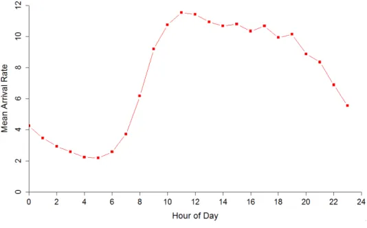
Figure 3.1: Arrival rate (number of arrivals per hour) vs. hour-of-day based on UNC ED 2012 data
Figure 3.2: Service rate (number of patients served per hour) per server under normal operating
conditions vs. hour-of-day based on UNC ED 2012 data
grows linearly from early morning to noon, and then stay constant at its peak for a couple hours during the daytime, and then linearly declines. We call the period during which the arrival rate stays constantly high the peak hours (9am to 5pm). Upon discussing with the ED staff we reached the agreement that at current stage it is only necessary to BeRT during the peak hours because the ED is usually not crowded in other time of the day. Since the arrival rate is approximately constant over time during the peak hours, we also assume thatλ(t) =λfor our problem. With the assumptions that all rates are constant over time we can re-express the previous formulation of our problem as below
min I(t):t∈[0,T]
Z T 0
x(t)dt
s.t. x(t) = sup0≤t
0≤tmax{x0+ Rt
0[λ−sµ(u)]du, Rt
t0[λ−sµ(u)]du}
,∀t∈[0, T],
Z T 0
I(t)dt≤δ,
I(t) = 0 or 1,∀t∈[0, T].
3.4 The Optimal Policy
and ts= max0≤t≤T{I(t) = 1}be the time BeRT ends. Thenµ(t) can be re-expressed as
µ(t) =
γ ift0 ≤t≤ts,
γ ift∈[0, T]\[t0, ts].
Also, the constraint on the total amount of time during which BeRT can be applied can be re-written as
ts−t0≤δ.
Hence the optimization problem becomes
min t0,ts
Z T 0
x(t)dt
s.t. x(t) = sup0≤t
0≤tmax{x0+Rt
0[λ−sµ(u)]du, Rt
t0[λ−sµ(u)]du}
,∀t∈[0, T],
µ(t) =
γ ift0 ≤t≤ts,
γ ift∈[0, T]\[t0, ts],
ts−t0 ≤δ, 0≤t0≤ts ≤T.
(3.1)
The next lemma further reduces the number of decision variables to only one.
Lemma 4. It is suboptimal to let t0> T −δ and ts−t0 < δ.
Although Lemma 4 is intuitive, it still requires a rigorous proof, which is provided in the Appendix. Based on Lemma 4, the problem reduces to finding only the optimal starting point for the BeRT interval, denoted byt∗0, which should be searched in [0, T −δ].
Theorem 4. The optimal policy π∗ that solves constrained problem (3.1) is to let t∗0 = 0 except when δ > t1 and t3 ≥0, we have t0∗= min{t2, t3, T−δ}, where
t1 =
x0
t2=
δ(sγ−λ)−x0
λ−sγ , and
t3 =
T−δ−(sγ−λs(γ−γ)(λ−sγ) )x0 2 +λ−sγsγ−λ
.
CHAPTER 4 Numerical Study
4.1 Introduction
As mentioned briefly in previous chapters, one proposed idea to reduce ED congestion is to predict whether or not a patient will eventually be admitted to the hospital upon or shortly after arrival and request a bed from the hospital at that time. We term this strategy early BeRT (bed request) or call-ahead. Calling ahead has the potential to significantly reduce the time an admitted patient occupies a bed since the hospital bed the patient will transfer to might already be available by the time the “admit” decision for the patient is given or at least would be available soon after. However, if the patient for whom an “admit” prediction is made ends up being discharged from the emergency department, that would mean that hospital resources were unnecessarily used to make the bed available, which would also turn into a problem between the emergency department and the hospital.
In this chapter, we will conduct numerical studies to evaluate the performances of several early BeRT heuristic policies using a discrete-event simulation model built for the UNC ED. The measurements we use to compare the efficacy of different heuristics are the long-run average length-of-stay, waiting time, and daily number of false early BeRTs. A good heuristic policy will balance the trade-off between the length-of-stay and waiting time, and daily counts of false early BeRTs. The primary purpose of performing the numerical studies is that we could identify heuristics that are easy to implement in a real ED setting and perform reasonably well.
context described above, here type-2 probability corresponds to an individual patient’s admission probability, parallel service option corresponds to requesting a hospital bed early on and starting the bed preparation process in parallel with serving the patient in the ED, and sequential service option corresponds to waiting until the patient finish being served at the ED to request a hospital bed, if the patient turns out to be an admit. Chapter 3, on the other hand, employs a fluid model approximation and constrains the option of early BeRT to a single time interval, for which the start and end times are determined by system parameters. We are also going to consider a heuristic policy that is motivated by this fluid model solution.
This chapter is organized as follows: First, we will discuss heuristic policies considered in this chapter. Second, we will describe the simulation model that we used to represent the UNC ED. Third, we will discuss our experimental setting and then present the results that we found by implementing the aforementioned heuristics on the simulation model.
4.2 Heuristic Policies
4.2.1 The Current System
The simulation model we use to approximate the UNC ED system was built using the patient data for calendar year 2012. From this point on, we refer to the simulation model under the 2012 operating condition the current system. In the current system, no early BeRT is implemented for any patient that visits the ED. We refer the policy that does not call ahead for anyone Hcurrent. In later sections, we will compare the performance of other heuristic policies toHcurrent and focus on how much improvement we can get for length-of-stay and waiting time, given certain tolerance for daily false call-aheads.
4.2.2 Fixed Threshold Policy (FT)
FT simply uses a constant threshold on the admission probability, denoted as T, to make a decision for calling ahead. When a patient enters service, one checks the patient’s probability of admission α, and calls ahead if and only if
whereT is a constant between 0 and 1.
4.2.3 Time-Dependent Threshold Policy (TT)
TT is a myopic policy that only takes into account the cost associated with one single patient, despite of the system’s state of crowding, where we use the cost structure described in Chapter 2. For a single patient, if one does not call ahead for a bed, the expected total cost incurred from the time when the patient enters service to the time the patient leaves the system is
Cw
1
γ1 + α
γ2
+αCs,
while if one chooses to make an early BeRT for the patient, the expected total cost is
Cw
1
γ1 + α
γ2
− α
γ1+γ2
+Cp.
TT says that to make an early BeRT for each individual patient if and only if
Cw
1
γ1 + α
γ2
− α
γ1+γ2
+Cp ≤Cw
1
γ1 + α
γ2
+αCs,
or equivalently,
α≥ Cp
Cs+γ1C+wγ2
. (4.1)
The policy can be time-dependent because both γ1 and γ2 can be dependent on time of day, and the patient type.
4.2.4 Census and Time-dependent Threhold Policy (CTT)
CTT chooses actions differently depending on whether the system has a queue or not. When the system has no queue, then CTT follows what TT does, i.e., to call ahead if and only if (4.1) holds.
2, except that the system does not have any arrivals from the beginning of time, but starts with a fixed number of customers to be served until empty. All the terminology and notations used in Chapter 2 carry over therein. For the clearing model, our objective is to minimize the total cost until the system is emptied by choosing which customers we apply the early BeRT option. The optimal policy we found there is to start early BeRT for the customer if and only if
nCw
α γ1+γ2
≥Cp−αCs,
wherendenotes the number of patients present in the system at the decision epoch andαdenotes the admission probability of the patient for whom we are making an admit decision. To apply the intuition of this formula in a real ED setting where there are multiple servers and random arrivals to the system, we replace n in the formula, which represents the number of customers left in the clearing model system at the decision epoch, by the expected number of patients that will be served until the queue is first emptied, denoted byne, given the current number of patients in the queue, denoted bym. Additionally, assuming the number of servers is denoted byK, then the service rate isK(γ1+γ2) instead of γ1+γ2.
It is straightforward to see that neis a function of m, and is also dependent on how one serves the patients because the total service time distribution for a patient is different if one chooses to early BeRT. That being said, we approximate the system behavior through a way which leads to CTT, which assumes that givenm, the current number of patients in the queue,neis approximately equal to the number of patients served until the queue reaches empty state for the first time with the system behaving as a M/G/1 queue, where the service time distribution is the same if early BeRT is applied to everyone being served during that cycle.
Using the well-known formula in classic queueing theory for the first-passage time from any statem to state 0 for a M/G/1 system with arrival rate λand mean service time τ we have that, one chooses to early BeRT for a patient with admission probability α when there are m patients in the queue if and only if
ne(m)Cw
α K(γ1+γ2)
where ne(m) = 1−λτm , and τ =
1 γ1 +
α γ2
−1
K−1. Let N denote the number of patients in the system, then m=N−K. By rearranging the terms and substituting it into the above formula we have
α≥ Cp
Cs+
Cw
γ1+γ2
m K(1−λτ)
.
Now we are one step away from formulating CTT. Notice that at this point, our policy is to call ahead if and only if
α≥ Cp
Cs+γ1C+wγ2
.
when there is no queue, orN ≤K. And to call ahead if and only if
α≥ Cp
Cs+
Cw
γ1+γ2
N−K K(1−λτ)
.
when there is a queue, orN > K.
However, we want to make CTT continuous in the sense that substituting N = K into the formula for the case whenN > K gives a threshold the same as that for the case whenN ≤K. To achieve this, we simply add a constant to the right hand side of the above formula, and thus CTT dictates that whenN > K,
α≥ Cp
Cs+
Cw
γ1+γ2
N−K K(1−λτ)
+
Cp
Cs+γ1C+wγ2 −1.
4.2.5 Constrained Fixed Threshold Policy (CFT)
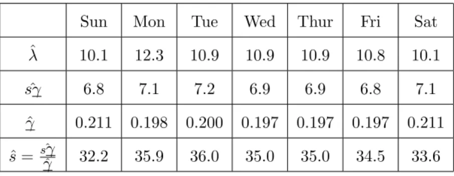
Keep in mind that the higher service rate as assumed in the fluid model is achieved, in a real ED setting, by calling ahead for a group of patients that are identified as to-be-admits. This is done by setting a threshold for admission, and categorize a patient to the admit group if and only if the patient’s admission probability, which is generated upon arrival in the simulation model according to certain distributions, exceeds the preset threshold. As mentioned briefly in Chapter 3, we are only going to implement early BeRT during the peak hours, which is taken to be 9am to 5pm based on Figure 3.1 where it is a period of time when the arrival rate seems to be constant over time. When implementing Theorem 3.4.1 shows that to the structure of the optimal policy depends on the values for x0, λ, s, γ, γ, and δ. We assume that x0 = 0, i.e., the number of patients in the queue at 9am, because before the peak hours the arrival rate is constantly small, which implies that there will not be much accumulation in the queue before 9am. We discussed the method of estimatingλand γ in Section 3.3. While here, since we have a simulation model that is validated using the 2012 UNC ED data, we use the simulation to re-estimate all the parameters in a similar vein. To be more specific, for the peak hours during each day of a week,λis taken to be the mean number of hourly total patient arrivals during the peak hours. γ is the inverse of the mean sojourn time (service + boarding) of all patients that entered service during the peak hours. Additionally, here we takesγ as the mean number of hourly total patient departures during the peak hours, and thus ˆs= sγˆˆγ.
Table 4.1 below shows the estimated λ,sγ,γ, anss using the simulation model under normal operating conditions (without call-aheads).
Sun Mon Tue Wed Thur Fri Sat
ˆ
λ 10.1 12.3 10.9 10.9 10.9 10.8 10.1
ˆ
sγ 6.8 7.1 7.2 6.9 6.9 6.8 7.1
ˆ
γ 0.211 0.198 0.200 0.197 0.197 0.197 0.211 ˆ
s= sγˆˆγ 32.2 35.9 36.0 35.0 35.0 34.5 33.6
Table 4.1: Estimated for 9am to 5pm
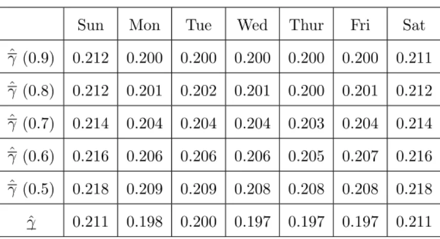
Once we fix the threshold for early BeRT, then one can estimateγ the same way as one estimates
γ.
Table 4.2 below shows the estimated γ under different thresholds for admission.
Sun Mon Tue Wed Thur Fri Sat
ˆ
γ (0.9) 0.212 0.200 0.200 0.200 0.200 0.200 0.211 ˆ
γ (0.8) 0.212 0.201 0.202 0.201 0.200 0.201 0.212 ˆ
γ (0.7) 0.214 0.204 0.204 0.204 0.203 0.204 0.214 ˆ
γ (0.6) 0.216 0.206 0.206 0.206 0.205 0.207 0.216 ˆ
γ (0.5) 0.218 0.209 0.209 0.208 0.208 0.208 0.218 ˆ
γ 0.211 0.198 0.200 0.197 0.197 0.197 0.211
Table 4.2: Estimatedγ under different admission thresholds for 9am-5pm
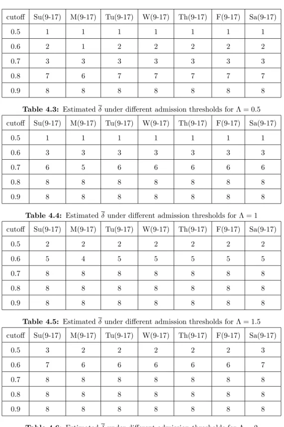
The estimation of δ takes a bit more effort. First, keep in mind that δ in our fluid model formulation represents the maximum amount of time one can use the maximum service rate. In a real ED setting, managers care about the number of false positive early BeRT per day, which we will use to determine δ. Additionally, δ is also dependent upon the admission threshold because the higher the threshold, the less patients we will categorize as admits, and the less false positives we will cause daily.
Let Λ denote the number of incorrect call-aheads the ED managers can tolerate per day. λ0
being the peak-hour number of incorrect call-aheads per hour, which is dependent on the cutoff for admission, then
λ0 =peak-hour number of incorrect call-aheads
=peak-hour number of arrivals per hour×impact×fp =λ×impact×fp.
those who have predicted admission probabilities no less than the BeRT cutoff. Consequently, we have
δ = Λ
λ0.
cutoff Su(9-17) M(9-17) Tu(9-17) W(9-17) Th(9-17) F(9-17) Sa(9-17)
0.5 1 1 1 1 1 1 1
0.6 2 1 2 2 2 2 2
0.7 3 3 3 3 3 3 3
0.8 7 6 7 7 7 7 7
0.9 8 8 8 8 8 8 8
Table 4.3: Estimatedδ under different admission thresholds for Λ = 0.5
cutoff Su(9-17) M(9-17) Tu(9-17) W(9-17) Th(9-17) F(9-17) Sa(9-17)
0.5 1 1 1 1 1 1 1
0.6 3 3 3 3 3 3 3
0.7 6 5 6 6 6 6 6
0.8 8 8 8 8 8 8 8
0.9 8 8 8 8 8 8 8
Table 4.4: Estimatedδunder different admission thresholds for Λ = 1
cutoff Su(9-17) M(9-17) Tu(9-17) W(9-17) Th(9-17) F(9-17) Sa(9-17)
0.5 2 2 2 2 2 2 2
0.6 5 4 5 5 5 5 5
0.7 8 8 8 8 8 8 8
0.8 8 8 8 8 8 8 8
0.9 8 8 8 8 8 8 8
Table 4.5: Estimatedδ under different admission thresholds for Λ = 1.5
cutoff Su(9-17) M(9-17) Tu(9-17) W(9-17) Th(9-17) F(9-17) Sa(9-17)
0.5 3 2 2 2 2 2 3
0.6 7 6 6 6 6 6 7
0.7 8 8 8 8 8 8 8
0.8 8 8 8 8 8 8 8
0.9 8 8 8 8 8 8 8
4.3 Simulation Model
This section discusses the simulation model that we employ to evaluate the efficacy of different heuristic policies in terms of their impact on reducing ED crowding. The simulation model is an extension of an early version, which was built and consistently refined by previous graduate students working on other projects related to UNC ED. Interested readers can refer to (Ahalt et al., 2016) for the first version of the simulation model and the project where it was used. Since many of our assumptions for the mathematical models are drawn from the 2012 UNC ED patient data, the earlier version of the simulation model needs to be updated so that the input parameters reflects the operating conditions at the ED during that time. The content of this section is organized as follows: First, input parameter analysis using the 2012 UNC ED data; Second, validation of the simulation model based on the 2012 UNC ED data.
The simulation model captures the patient flow going through the UNC ED at a highly detailed level, which can be viewed as a queueing process that consists of five components: arrival, triage, service, boarding, and departure. Figure 4.1 gives a general overview of this queueing process:
Figure 4.1: Patient flow at The ED
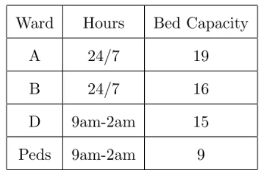
however, be admitted to ward A or B during after hours. Table 4.7 summarizes the hours of four wards’ and bed capacities.
Ward Hours Bed Capacity
A 24/7 19
B 24/7 16
D 9am-2am 15
Peds 9am-2am 9
Table 4.7: Ward hours and bed capacity
ESI measures the severity of a patient’s medical condition. There are five ESI levels ranging from 1 to 5 with lower numbers indicating higher criticality. Finally, there are two disposition categories: admitted and discharged. Admitted patients will be hospitalized after their ED visits while discharged patients leave the hospital system immediately after their ED visit.
Arriving patients join the queue for triage where they get assigned an ESI level. There are typically two triage nurses at triage and their service times are assumed to follow i.i.d. triangular distribution. We make this assumption on the distribution and its parameters based on experience of ED managers that we collaborate with since our data does not have triage times.
After triage, patients join a queue to wait for ED bed assignment. In the simulation model, we do not explicitly model the attending physicians or any other medical personnel. Instead, we regard each ED bed as a server. The first part of service a patient will receive at the ED starts when the patient is assigned to an ED bed and ends when a disposition decision is made for him/her.
4.3.1 Input Analysis
I performed input parameter estimations using the 2012 UNC ED patient data. The information available for each visit includes the patient’s age, gender, ESI, disposition, arrival time, ED bed assignment time, disposition decision time and departure time. Entries with missing data or out-of-order time stamps are deleted. The cleaned data has approximately 56,000 entries (corresponding to 56,000 patient visits).
As mentioned earlier, the parameters that needed to be estimated are the arrival rates, service time, and boarding time distributions. Arrival rates are dependent on hour of the day, day of the week, and patient type broken down by age (adult vs. pediatric), ESI and disposition (admitted vs. discharged). Figure 3.1 displays the hourly average arrival rate for all patient types combined. Note that this is just a demonstration of the time varying nature of the arrival rate. In the actual simulation model the patients arrive according to time-varying arrival rates based on their types. The service times are dependent on hour of the day and patient type broken down by age (adult vs. pediatric) and ESI. Lastly, boarding times are dependent on hour of the day and patient type broken down by age (adult vs. pediatric), ESI and disposition (admitted vs. discharged).
and shape parameters. EXP stands for the Exponential distribution where the parameter is the mean. N stands for the Normal distribution where the first and second parameters represent the mean and standard variance. And finally, we use the notation EXP(pN(µ1, σ1) + (1−p)N(µ2, σ2)) to represent a random variable Y, such that logY follows a mixed Normal distribution. To be more specific, with probabilityp, logY follows N(µ1, σ1), and with probability 1−p, logY follows N(µ2, σ2). Also in the tables, p-value is based on KS test that examines the closeness between the fitted and empirical distribution.
Patient type Hour Service time distribution P-value MSE
A1 0-23 1+GAMM(101,0.952) >0.15
A2 2-9 1+GAMM(185,1.37) 0.022 0.00443
A2 9-14 4+ERLA(125,2) 0.027 0.00183
A2 14-20 EXP(0.68N(5.45,0.54)+0.32N(5.14,0.24)) >0.15
A2 20-2 EXP(0.97N(5.41,0.82)+0.03N(2.63,0.90)) 0.060
A3 2-9 EXP(0.9N(5.43,0.60)+0.1N(4.31,0.96)) 0.059
A3 9-20 1+ERLA(83.9,3) ¡0.01 0.00026
A3 20-2 EXP(0.92N(5.38,0.58)+0.08N(4.23,1.02)) >0.15
A4 2-9 1+GAMM(95.5,1.49) 0.090
A4 9-14 1+GAMM(90.4,1.47) 0.070
A4 14-20 1+GAMM(80.6,1.54) 0.134
A4 20-2 1+ERLA(71.3,2) 0.028 0.00082
A5 0-5 1+EXP(105) >0.15
A5 5-23 EXP(0.8N(4.00,0.84)+0.2N(2.96,1.06)) >0.15
Patient type Hour Serivce time distribution P-value MSE
P1 0-23 2+EXP(78.7) >0.15
P2 2-9 7+WEIB(240,1.06) >0.15
P2 9-14 6+WEIB(305,1.38) >0.15
P2 14-2 EXP(0.95N(5.25,0.86)+0.05N(2.82,0.86)) 0.116
P3 0-23 2+GAMM(79.7,2.33) 0.050 0.00026
P4 0-23 1+GAMM(50.9,2.37) 0.095
P5 0-23 1+GAMM(36.8,2.27) >0.15
Table 4.9: Service time distributions for pediatric patients
Patient type Hour Boarding time distribution P-value MSE
AA1 2-9 17+WEIB(122,0.935) >0.15
AA1 9-12 WEIB(180,1.05) >0.15
AA1 20-2 WEIB(153,0.955) 0.0423 0.00706
AA2 5-16 EXP(0.95N(5.47,0.634)+0.05N(3.77,1.31)) >0.15
AA2 16-5 EXP(0.61N(5.03,0.440)+0.39N(5.20,1.22)) >0.15
AA3 5-16 EXP(0.93N(5.50,0.563)+0.07N(4.43,0.998)) >0.15
AA3 16-5 EXP(0.63N(5.05,0.419)+0.37N(5.37,1.00)) >0.15
AA45 0-5 2+GAMM(188,1.18) 0.069
AA45 5-0 11+ERLA(99.2,2) >0.15
AD12 3-8 1+943BETA(0.183,2.11) 0.001 <0.001
AD12 8-3 WEIB(34,0.616) <0.01 0.00328
AD3 5-11 WEIB(33.6,0.663) <0.01 0.00693
AD3 11-5 WEIB(25.1,0.657) <0.01 0.00256
AD4 2-9 EXP(25.6) <0.01 0.00583
AD4 9-2 EXP(19.9) <0.01 0.00061
AD5 2-9 EXP(23.1) 0.046 0.00997
AD5 9-2 EXP(15.9) <0.01 0.00435
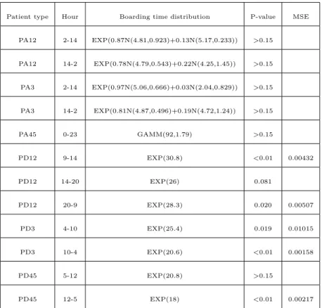
Patient type Hour Boarding time distribution P-value MSE
PA12 2-14 EXP(0.87N(4.81,0.923)+0.13N(5.17,0.233)) >0.15
PA12 14-2 EXP(0.78N(4.79,0.543)+0.22N(4.25,1.45)) >0.15
PA3 2-14 EXP(0.97N(5.06,0.666)+0.03N(2.04,0.829)) >0.15
PA3 14-2 EXP(0.81N(4.87,0.496)+0.19N(4.72,1.24)) >0.15
PA45 0-23 GAMM(92,1.79) >0.15
PD12 9-14 EXP(30.8) <0.01 0.00432
PD12 14-20 EXP(26) 0.081
PD12 20-9 EXP(28.3) 0.020 0.00507
PD3 4-10 EXP(25.4) 0.019 0.01015
PD3 10-4 EXP(20.6) <0.01 0.00158
PD45 5-12 EXP(20.8) >0.15
PD45 12-5 EXP(18) <0.01 0.00217
Table 4.11: Boarding time distributions for pediatric patients
4.3.2 Calibration and Validation
the simulation model and that of the original data, we will be able to see whether our assumptions on the bed capacities, arrivals, work together perfectly to produce a simulation model that mimics the behavior of the original system in 2012.
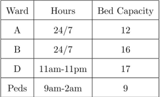
One important thing to note here is that in the simulation model, the notion of servers is modeled as ED bed resources. However, in the data we have available, the beginning of service time is defined as the first time that a patient was attended by an ED provider, which is not necessarily the first time that the patient gets assigned an ED bed. Because of the discrepancy, we had to calibrate bed capacity to achieve a match between the output of the simulation model and that estimated from the data for the three time measurements we consider. The resulting bed capacity is different from that of Table 4.7, and is summarized in Table 4.12.
Ward Hours Bed Capacity
A 24/7 12
B 24/7 16
D 11am-11pm 17
Peds 9am-2am 9
After the aforementioned calibration, we arrive at a simulation model that accurately represent the operating condition of the UNC ED in 2012, as measured by service time, boarding time, and sojourn time. Figure 4.2 shows the result.
Figure 4.2: Sojourn Times Validation
4.4 Numerical Study
A natural assumption on the admission probability distribution would be to use the empirical distributions, as estimated by our APT. To be more specific, we applied APT on the 2012 UNC ED data, obtained a predicted admission probability for each individual patient, and fit an empirical distribution for each individual patient group broken down by their acuity, age (adult vs. pediatric), and disposition category (admit vs. discharge). According to the histograms of patients’ predicted admission probabilities, we observe only a few distinct bars in all the histograms, meaning that for each individual patient group, the predicted admission probabilities tend to occur at a few distinct values most frequently. Based on this observation, for the empirical distributions we fit, we assumed uniform distributions between those most frequent values.
to each point in the plots. Notice that in the figures we also provide the 95% confidence interval (CI) bands around the mean values.
Figure 4.3: Length-of-stay (LOS) under CTT and FT
Figure 4.4: Length-of-stay (LOS) under CTT and TT
4.5 Discussion
As is shown in Figure 4.3 through Figure 4.5, we looked at cases where the daily counts of false early BeRTs are between the value of 0 and 3. The general pattern is that the higher the daily counts of false positives, the larger the improvement on LOS and waiting time one achieves. Under the current system, the average LOS is 358min. It is evident that as the variances of the distributions decreases, larger improvement on the LOS can be expected given certain level of daily false positives. When one allows for 3 daily false positives, the heuristics result in a LOS in the range of 346min to 347min, corresponding to 11 to 12min reduction.
CHAPTER 5
Impact of Census on Emergency Department Providers’ Triage and Admission Decisions
5.1 Introduction
Emergency Departments (EDs) are busy places. In 2015 there were 136.9 million ED visits in the United States. This high volume often leads to ED crowding that has been associated with numerous negative patient outcomes including delays in lifesaving care that result in increased mortality and low patient satisfaction (George and Evridiki, 2015), (McCarthy et al., 2009), (Richardson et al., 2006), (McCusker et al., 2014).
It has been suggested that crowding of the emergency department can lead to difficulties with clinician decision-making and potentially impact equity in care (Hwang et al., 2011). Two such vital decision points that are tied to care quality and equity are the triage level assignment decision made by nursing staff and the disposition decision made by providers.
Nationally, emergency departments represent a significant source of hospital admissions ac-counting for nearly all the growth of hospital admissions in recent years (Morganti et al., 2013). The decision to admit a patient is made by emergency providers based upon available individual patient data, however recent research suggests that this decision may also be influenced by crowding of the ED itself (Gorski et al., 2017). This recently published study at a single academic medical center finds a statistical association between the likelihood of hospital admission and increased ED census. It was suspected that as EDs become busier there is a cognitive offloading that occurs for the physician by admitting patients rather than spending time and mental energy arranging safe discharges for patients who may be in a “gray area”.