Technical.Report.Final.Minge.Jiang.20191213.pdf

(1)

i

DILUTE SPECIES TRANSPORT IN NON-NEWTONIAN, SINGLE-FLUID, POROUS MEDIUM SYSTEMS

Minge Jiang

A technical report submitted to the faculty at the University of North Carolina at Chapel Hill in partial fulfillment of the requirements for the degree of Master of Science in Environmental

Engineering in the Department of Environmental Sciences and Engineering in the Gillings School of Global Public Health.

Chapel Hill 2019

(2)

(3)

iii ABSTRACT

Minge Jiang

(Under the direction of Cass T. Miller)

(4)

iv

ACKNOWLEDGEMENTS

On my way here today to finish this report, I have a lot of people whose support, advice, and help have been fundamental parts of my accomplishments in life. First of all, I want to sincerely thank my advisor, Dr. Cass T Miller, who gave me plenty of support, patience, guidance, and help during the last one and a half years at UNC-CH. He was incredibly patient to edit my writing repeatedly, helped me to improve my work, explained obscure professional terms to me, taught me theoretical essential knowledge about groundwater hydrology, and guided me into numerical methods and the scientific computation world. Without his help, I could not have finished this final report ahead of the original plan.

Furthermore, I would like to give special thanks to the members of Dr. Miller’s research group: Christopher Bowers, Brittany Shepherd, Kelsey Bruning, Timothy Weigand, Christopher Fowler, and Pamela Schultz, who have helped me in areas ranging from housing to classes to research work throughout the time I have spent here. I am especially grateful to Christopher Bowers; without his support to teach me about the experiments and simulations, and his explanations of many hard-to-understand theories, I would not have been able to complete my report, or indeed to make it through this year and a half at all. I want to thank my committee members, Dr. Orlando Coronell and Dr. Jason Surratt; their classes were insightful and informative. It has been my honor to work with all of them.

(5)

v

LIST OF FIGURES

Figure 1. Schematic of Column-Pump Porous Medium System ... 20

Figure 2. Schematic of Domain System ... 28

Figure 3. DIW Tracer Tests Breakthrough Curve ... 40

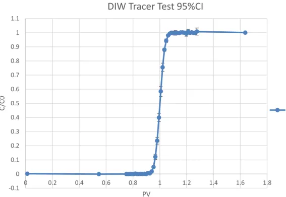
Figure 4. DIW Tracer Tests 95% Confidence Interval Breakthrough Curve ... 40

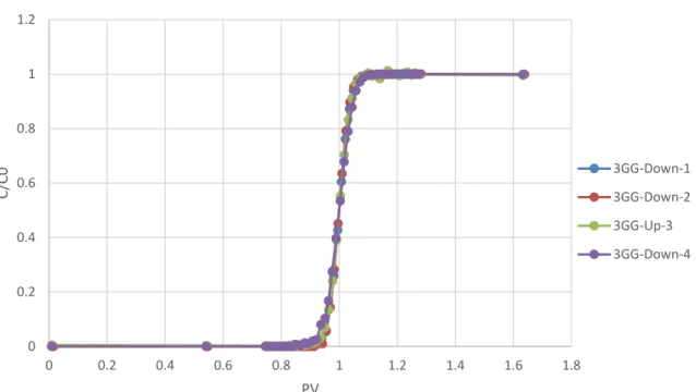
Figure 5. 0.3% Guar Gum Tracer Tests Breakthrough Curve ... 41

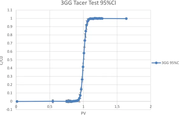
Figure 6. 0.3% Guar Gum Tracer Test 95%CI ... 42

Figure 7. 0.5% Guar Gum Breakthrough Curve ... 42

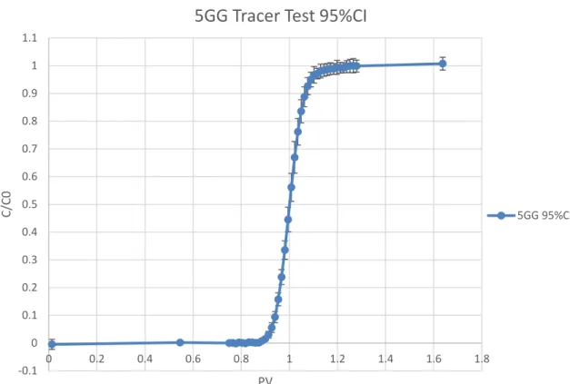
Figure 8. 0.5% Guar Gum Tracer Test 95% CI ... 43

Figure 9. Post-DIW Tracer Test Breakthrough Curve ... 44

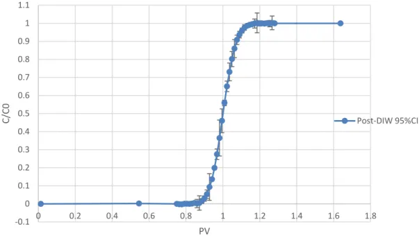
Figure 10. Post-DIW Tracer Test Breakthrough Curve 95% CI ... 44

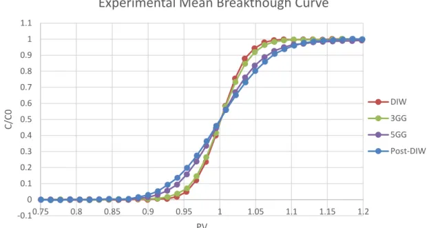
Figure 11. Experimental Mean Breakthrough curve comparison ... 45

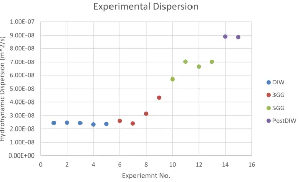
Figure 12. Experimental Hydrodynamic Dispersion Comparison ... 46

Figure 13. Experimental Mean Dispersion 95% CI ... 47

Figure 14. Experimental Breakthrough Curve Fitting ... 48

Figure 15. Analytical Hydrodynamic Dispersion Model Sensitivity ... 49

Figure 16. Experimental Pe Number ... 50

Figure 17. Picture of the Domain from ParaView ... 52

Figure 18. Pressure Drop Varies with Different Spheres and Blocks ... 55

Figure 19. Pressure Drop for 0.3% Guar Gum at v = 0.00005 m/s ... 55

Figure 20. Average Pressure Drop per Length for 0.3% Guar Gum at v = 0.00005 m/s ... 56

Figure 21. REV With Respect to Conductivity Under Different Domain Systems ... 57

Figure 22. Simulation Breakthrough Curve at v=0.0005m/s, DT=2.05E-10 ... 58

Figure 23. Simulation Breakthrough Curve at v=0.00005m/s, DT=2.05E-10 ... 59

Figure 24. Simulation Breakthrough Curve v=0.000005m/s, DT=2.05E-10 ... 59

Figure 25. Simulation 0.3% Guar Gum at v=0.0005m/s Breakthrough Curve ... 60

Figure 28. Simulation Hydrodynamic Dispersion at different velocities ... 62

Figure 29. Simulation Hydrodynamic Dispersion at Different DT ... 63

(8)

viii

LIST OF TABLES

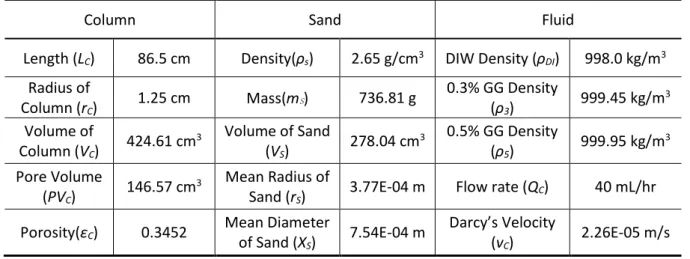
Table 1. Column and Sand Data ... 39

Table 2. Experiment Reynolds Number ... 50

Table 3. Packed Domain Systems Data ... 51

(9)

ix

LIST OF NOMENCLATURE

Roman Letters

𝐴 Area [L2]

C Concentration [M/L3_] 𝐶₀ Initial concentration [M/L3]

𝐷_𝑙 Longitudinal hydrodynamic dispersion coefficient [L2/T] 𝐷_𝑚 Molecular diffusion coefficient [L2/T]

𝑔 Gravity acceleration [L/T2_] 𝐾 Hydraulic conductivity [L/T]

𝑙 Linear coordinate along the flow direction [L] 𝐿 Length [L]

𝑚 Cross power model fitting parameter M Mass [M]

𝑛 Cross power model fitting parameter 𝑁𝑠 Sphere number

𝑃 Pressure [M/LT2] 𝑄 Flow rate [L3/T] 𝑟 Radius [L] 𝑡 Time [T]

T Relative concentration in OpenFOAM simulation 𝒖 Flow velocity tensor with the order of two [L/T] 𝑣 Darcy velocity [L/T]

𝑣̅ Average Darcy velocity [L/T] V Volume [L3]

𝑋 Mean diameter of particles [L] Greek Letters

𝛼 Courant number

𝛼𝑙 Dispersivity of the porous medium [L]

(10)

x 𝜇 Dynamic viscosity [M/LT]

𝜇₀ Dynamic viscosity at zero shear rate [M/LT] 𝜇𝐼𝑛𝑓 Dynamic viscosity at infinite shear rate [M/LT]

𝜇𝑙𝑜𝑔 Lognormal mean

ν Kinematic viscosity [L2_/T]

ν₀ Kinematic viscosity at zero shear rate [L2/T] ν_∞ Kinematic viscosity at infinite shear rate [L2/T] 𝜌 Density [M/L3]

σ2 _{Lognormal distribution variance}

τ Shear stress [M/LT2_]

𝜔 Specific thermodynamic work per unit mass Mathematical Letters

𝐶

𝐶₀ Relative concentration

𝑑ℎ Hydraulic head loss [L]

𝑑ℎ

𝑑𝐿 Hydraulic gradient

erfc Complementary error function 𝑔𝑟𝑎𝑑 Gradient

MASS Mass [M] Pe Peclet number

𝑃𝑉 Number of pore volume passed through 𝑃𝑉_𝐶 Pore volume of the column [L3]

Re Reynolds number

Re0 Reynolds number at zero shear rate

ReInf Reynolds number at infinite shear rate

(11)

xi

LIST OF ABBREVIATIONS

1003 Resolution blocks level at x-y-z as 120×100×100 2003 Resolution blocks level at x-y-z as 240×200×200 3003 _{Resolution blocks level at x-y-z as 360×300×300} 4003 _{Resolution blocks level at x-y-z as 480×400×400} 5003 Resolution blocks level at x-y-z as 600×500×500 3GG 3% by mass guar gum solution

5GG 5% by mass guar gum solution 95% CI 95% Confidence interval DIW Deionized water

EPA United States Environmental Protection Agency EIA United States Energy Information Administration OpenFOAM The Open Source Field Operation and Manipulation REV Representative Elementary Volume

(12)

1

Chapter 1: Introduction

Motivation

Global primary energy consists of petroleum, natural gas, coal, nuclear energy and

renewable sources. In 2018, the world primary energy production grew by 2.8%

compared to the primary energy production in 2017, and the U.S. and China together

made up 54% of this growth [1]. Global primary energy consumption grew 2.9% in

2018, the fastest growth rate since 2010, mainly driven by natural gas, which

accounted for more than 40% of the total increase. Approximately 85% of this

consumption was in the form of fossil fuels. Global natural gas production and

consumption increased by 5.3% and 5.2% in 2018, respectively, and nearly half of the

production growth occurred in the U.S. [2]. In the U.S., fossil fuel accounted for

approximately 80% of energy consumption in 2018, with 31% of energy consumption

provided by natural gas [3].

Fossil fuels will continue to play an important role in energy production and

consumption in the coming decades around the world, even as the transition to

renewable sources of energy continues [4]. A long-term projection report indicates

that, without a dramatic shift in current climate policies, global energy consumption

will grow 20%-30% from now through 2040, mainly driven by fossil fuels, especially

natural gas [5]. Based on the evaluation of Tong et al. [6], in 2018, the world

recoverable conventional oil and natural gas resources are 535 billion tons and 588.4

trillion cubic meters, respectively. In 2016, Wang et al. [7] assessed total global

(13)

2

tight geological formations with low permeability, at an astonishing 442.1 billion tons

and 227 trillion cubic meters, respectively. Both of these estimates document

abundant conventional and unconventional hydrocarbon resources globally.

Hydrocarbon reserves are stored in two different ways and require different

extraction technologies. The hydrocarbon resources that come from

high-permeability formations, such as large fractures in sandstones or limestones, can be

easily obtained by standard well and pumping technologies and are called

conventional hydrocarbons. Alternatively, unconventional hydrocarbons are usually

trapped in tight geological formations, such as shales, with low permeability and

porosity, and cannot be extracted from the deposit by utilizing simple drilling and

production techniques. The latest data shows that from 2016 to 2017, the proven

crude oil reserves in the U.S. increased 19.5% to 39.2 billion barrels (bbl), equivalent

to 5.73 billion tons. Moreover, the proven natural gas reserves increased by 36.1% to

464.3 trillion cubic feet (Tcf), equivalent to 13.15 trillion cubic meters (Tcm). It should

be noted that the share of shale gas grew from merely 13.5% in 2008 to 66% in 2017,

or about two-thirds of the total proven natural gas reserves [8]. The increasing

importance of shale gas, or unconventional natural gas, is an influential trend in

energy production and consumption, especially in the U.S.

Hydraulic fracturing, also known as fracking, is one of the most important extraction

technologies in the fossil fuel industry since the late 1940’s, and the primary method

for unconventional hydrocarbon resource exploitation. Hydraulic fracturing has

developed dramatically in the past few decades to enhance the production of

(14)

3

economically from unconventional reservoirs [9]. From 2004 to 2019, the production

of shale gas in the U.S. grew from about 0.8 billion cubic feet (22.6 million cubic meters)

per day to 3.0 billion cubic feet (85.0 million cubic meters) per day [10]. Though it is a

fossil fuel that produces greenhouse gas when burned, natural gas emits

approximately 50% less CO2 than coal and about 28% less CO2 than oil per unit of

energy production [11], and it emits far less sulfur dioxide (SO2), and nitrogen oxides

(NOx)than either coal or oil. The projection from EIA [12] in 2019 shows that, without

significant changes to clean energy policies, annual energy-related CO2 emission will

fall 4% to about 5 billion metric tons from 2018 to 2050 in the U.S. as a result of a

migration from the consumption of coal and petroleum to natural gas.

The practice of hydraulic fracturing is generally combined with horizontal drilling

techniques, and the process includes several steps: (1) drilling and construction of

wells vertically and then horizontally to reach the hydrocarbon reservoirs far below

the surface; (2) injection of pressurized hydraulic fluids into the wells to exceed the

fracture gradient of the shale needed to form permeable cracks for fluids; (3)

production of petroleum and natural gas from the wells; and (4) maintenance of the

well system and treatment and disposal of fluid waste [13]. Although hydraulic

fracturing dominates the global production of natural gas, it has been a controversial

technique since its introduction. Concerns about the potential impacts of hydraulic

fracturing on the environment, especially on groundwater and surface water quality,

have drawn considerable attention from the research community, the public, and

government [14–20].

(15)

4

fracturing fluids applied during the fracturing process on subsurface water quality.

Hydraulic fracturing fluids are often a type of non-Newtonian fluid, which consists of

sand, large amounts of water, and a mixture of toxic chemicals. Specific concerns

related to the hydraulic fracturing process include leakage of fluids, unrecovered fluids

seeping down into the reservoirs, and potential transport of toxic chemicals into

groundwater systems, the ecosystem, and water supplies [21]. Such contamination

from hydraulic fracturing is extremely difficult to identify and remediate. Many open

research questions must be resolved before the environmental risks resulting from

hydraulic fracturing can be clearly understood. Included in these open questions are

the mechanics of transport phenomena in non-Newtonian fluids, which are the

majority of fluids used in hydraulic fracturing.

Fluid characterization depends on a number of variables. Different fluids or materials

have their own behavior patterns when subjected to stress, shear rate, velocity,

deformation, and flow. Based on their viscosity characteristics, fluids can be classified

as Newtonian or non-Newtonian fluids. Newtonian fluid remains at a constant

viscosity as a linear function of shear stress and shear rate; water and gasoline are two

examples. Non-Newtonian fluids are a group of materials, such as biological fluids,

aqueous guar gum solutions, and suspensions, whose viscosity characteristics do not

follow the classic Newtonian model [22]. As compared to Newtonian fluids, the

viscosity of non-Newtonian fluids [23] has a non-linear correlation between the shear

rate and shear stress. When the derivative of the shear stress with respect to the

applied shear rate is positive, the fluid is defined as a shear-thickening fluid, for which

(16)

5

of the shear stress with respect to applied shear rate is negative, the fluid is called a

shear-thinning fluid, for which the viscosity decreases as the shear rate increases.

In fluid mechanics, hydrodynamic dispersion is a factor that has been applied to

describe the transport of solutes in fluids. In the 1950s, Dr. Geoffrey Ingram Taylor

[24–26] published several papers about soluble matter dispersion in Newtonian fluids

flowing through a tube under certain fluid conditions. Taylor derived a classic

hydrodynamic model, known as the Taylor dispersion model. The Taylor dispersion

model has been proven efficient to fit Newtonian fluids [27–29]. However, because of

the unstable viscosity of non-Newtonian fluids, the Taylor dispersion model cannot

accurately describe the behavior of Newtonian fluids or species transport in

non-Newtonian fluids in porous media. The nature of species transport and dispersion in

non-Newtonian fluids remains unclear, and additional research is warranted. The

standard hydrodynamic dispersion model [30] from Taylor is based on mass

conservation equations and simulates the behavior of species in Newtonian fluids;

however, the hydrodynamic dispersion model for non-Newtonian fluids is uncertain,

and this work aims to narrow this knowledge gap in non-Newtonian fluids. Utilizing

the continuum method and the representative elementary volume concept, one can

observe variations in species dispersion in a non-Newtonian fluid in porous media at

the microscale level. These observations can then inform macroscale models of such

systems. Promoting such fundamental understanding would enable advances in

models used in a variety of fields including: hydrocarbon reservoir engineering,

groundwater hydrology, chemical processing, and other areas in which flow

(17)

6 Goal and Objectives

The goal of this work is to analyze dispersion of a dilute species in a non-Newtonian

fluid for single-fluid-phase transport in a porous media system. The specific objectives

of this work are: (1) to observe dilute species transport in an experimental porous

media system that includes a non-Newtonian fluid; (2) to mathematically model

species transport at the microscale for systems similar to those investigated

experimentally; and (3) to compare experimental observations and simulated

(18)

7

Chapter 2. Background

Natural Gas

Natural gas is one of the most common fossil fuels, naturally occurring deep beneath

the surface of the earth. Like other fossil fuels, natural gas is made up of remnants of

processes occurring under immense pressure and heat below the earth’s crust for

millions of years. Natural gas [31] consists of many different hydrocarbons, carbon

dioxide, nitrogen, and water vapor, but the primary component of natural gas is

methane (CH4). Natural gas that is found in large fractures in permeable formations is

called conventional natural gas, and natural gas that is found in fine-grained shale

formations with low permeability is called unconventional natural gas, or shale gas.

Natural gas occurrence is usually associated with petroleum deposits. In the 19th

century, natural gas was considered a by-product of crude oil extraction and was

burned off as waste from the petroleum field. However, in 2018, natural gas

contributed 32% of U.S. primary energy production [32], a figure that keeps growing.

With new extraction techniques and discoveries, the expansion of natural gas

production, and especially the dramatic rise in shale gas production has remapped the

U.S. energy landscape and turned the U.S. from a net energy consumer into a net

producer.

Many qualities of natural gas make it an economical and relatively clean energy source.

Natural gas has a higher caloric value (12,500 kcal/kg) than fuel oil (9,250 kcal/kg) or

brown coal (3,500 kcal/kg) under standard conditions [33]. Natural gas also has fewer

undesirable by-products emitted on combustion per unit energy than crude oil or coal

(19)

8

greenhouse effect of methane [36], the simplest alkane and principal component of

natural gas, and the leakage of natural gas from infrastructure [35] make its use

controversial with regard to climate change and global warming, natural gas is still a

relatively abundant, economical, efficient, and environmentally friendly fossil fuel

worldwide [34,37]. Natural gas is widely used as a fuel for homes, power plants,

industry, and automobiles. The typical efficiency of converting heat energy into

electrical power in a power plant is 60% for a natural gas combined-cycle power plant,

42% for a petroleum-fired power plant, and 33% for a coal-burning power plant [34].

At the end of 2017, the net increase in proved natural gas reserves in the U.S. was

123.2 Tcf, about 3.49 trillion cubic meters (Tcm); this was a new record of total proved

natural gas reserves, and the share of proved shale gas reserves increased to 66% of

total U.S. proved natural gas reserves [8].

Shale gas trapped in a shale deposit or formation has become the primary source of

natural gas production in the U.S. this century [38–40]. A shortage of crude oil and

conventional natural gas in the late 1960s, along with an evolution in extraction

methods made shale gas a significant energy source in fossil fuel production and

consumption worldwide. Technological advancements made the extraction of shale

gas economically viable. As one of the countries with the greatest proved natural gas

reserves, the U.S. has a large amount of stored natural gas that has not yet been

extracted. Prior to a few decades ago, these shale gas reservoirs were considered

uneconomic targets, requiring difficult procedures to access. However, due to the

development of hydraulic fracturing, these reservoirs are now both accessible and

(20)

9

gas production in the U.S. in 2017 [41]. Since extraction technology for natural gas

hydrates, also known as methane clathrate, is still evolving, shale gas will play a

significant role in the area of natural gas resources in the near future. Hydraulic

fracturing technology is becoming increasingly important, and it is indispensable for

exploiting shale gas reservoirs in the natural gas industry.

Hydraulic Fracturing

Hydraulic fracturing has become prevalent in crude oil and natural gas engineering in

recent decades. Hydraulic fracturing [42] is an established and rapidly advancing

technology that injects pressurized hydraulic fracturing fluids into targeted rock

formations through production wells to create fractures and maximize productivity of

petroleum and gas. Hydraulic fracturing forms cracks in permeable formations with

fine grains, props these fractures open using sand or silica, and improves the

permeability of tight shales artificially, allowing shale gas or petroleum to flow more

easily out of the shale than before.

Horizontal drilling is a procedure that follows vertical drilling down into the subsurface.

The horizontal portion of a well allows for a greater extent of a gas-containing region

to be in close contact to the well, reducing transport distances needed for effective

production. Hydraulic fracturing contributed 67% of the natural gas production and

51% of crude oil production in the United States in 2015, (EIA [43,44]). Since most of

the shallower and more-accessible oil- and natural gas-bearing rock formations have

already been exploited, hydraulic fracturing allows fossil-energy-mining technology

deep into production formation layers previously considered uneconomic. Along with

(21)

10

spread as a popular technique to help the world access existing energy reserves.

The hydraulic fracturing process includes well construction, water acquisition,

chemical mixing, pressurized injection, oil or natural gas extraction, and wastewater

disposal and reuse [13]. Hydraulic fracturing fluids are injected under high pressure to

open fractures in tight formations. The composition of fracking fluids varies with

different types of fracturing, usually consisting of water, proppants which are solid

materials such as sand, ceramic, and silica, and specific chemical additives, such as gels,

guar gum, biocides, emulsifiers, and friction reducers. Industrial practice tends to

choose more viscous fluids to carry more proppants, and such fluids are often

non-Newtonian fluids. Some of the components of hydraulic fracturing fluids are

biologically toxic, and the behavior of non-Newtonian fluids is difficult to model and

predict.

The advent and rapid development of hydraulic fracturing has drawn substantial

attention and debate from environmentalists, scientists, government, and the general

population. Due to the intricacy of unconventional reservoirs and geological

conditions, and the unclear attributes of hydraulic fracturing fluids, concerns have

been raised regarding the risk posed by the initiation and propagation of fractures in

shale formations and the potential resultant threats to groundwater aquifers. The

possible environmental hazards of hydraulic fracturing include substantial water use,

leaks and spills of hydraulic fracturing fluids, potential transport of fluids into

groundwater resources, and other risks associated with operations and extractive

activities [45,46]. Although there has been tremendous crude oil and natural gas

(22)

11

hydraulic fracturing techniques and applications, this process receives relatively little

regulatory surveillance, and the impacts of hydraulic fracturing on surface water

sources and groundwater remain unclear and infrequently studied.

In addition to lack of monitoring and regulation, scientific issues remain to be resolved

before a mature level of understanding is achieved. One of these issues is related to

the flow of non-Newtonian fluids, which are the typical hydraulic fracturing fluids,

through porous media. Non-Newtonian flow through a porous medium system is

often modeled using Darcy’s law, which is not strictly applicable because it does not

account consistently for the relationship observed between shear stress and shear

rate that typifies a non-Newtonian fluid. Furthermore, the transport of individual

dilute species in non-Newtonian fluids, such as is typical of many of the species of

environmental concern, is also not well understood.

Non-Newtonian Fluids

In fluid mechanics [47], the force applied to a fluid parallel to the direction in which

the fluid is moving per unit area is known as the shear stress (τ) [M/LT2_]._Dynamic

viscosity (µ) is defined as the deformational resistance of a fluid to applied shear stress.

When the shear stress exerted on a fluid is linearly proportional to the shear rate (𝑑𝑣_𝑑𝑦),

the viscosity of the fluid is constant, and the fluid is said to be Newtonian. This

relationship can be formulated as Eq. (1).

𝜏 = 𝜇𝑑𝑣

𝑑𝑦 (1)

(23)

12

The viscosity of Newtonian fluids remains constant at a given temperature, which

means it is easy to measure the dynamic viscosity for such a fluid. Common Newtonian

fluids include water, alcohol, gasoline, and mineral oil.

Fluids that do not follow Newton’s law of viscosity are known as non-Newtonian fluids.

Although many fluids are assumed to be Newtonian fluids for practical use,

non-Newtonian fluids are more common and have very different behavior and properties

than Newtonian fluids. In contrast to Newtonian fluids, the viscosity of a

non-Newtonian fluid varies as a function of the applied shear stress or force. The behavior

of a typical Newtonian fluid, such as water, depends on pressure and temperature.

The behavior of a non-Newtonian fluid changes with flow conditions as a result of the

dependence of dynamic viscosity on the rate of strain, in addition to the dependence

on pressure and temperature. A typical example of a non-Newtonian fluid is ketchup:

if one squeezes and shakes a ketchup bottle, it will pour out significantly faster than

just turning over the bottle to wait for it to drop, because the ketchup’s viscosity is

altered when a stress is applied to it.

Non-Newtonian fluids can demonstrate various trends in dynamic viscosity as a

function of the deformation rate, time, and composition, and there are four types of

non-Newtonian fluids [48]. When the viscosity of a non-Newtonian fluid decreases

with the increased shear rate, the fluid is called a shear thinning fluid, such as ketchup;

when the viscosity increases with the increased shear rate, the fluid is called shear

thickening fluid, such as oobleck. For time-dependent viscosity, if the viscosity of the

fluid decreases with the length of time that stress is applied, then the fluid is defined

(24)

13

the length of time that stress is applied, the fluid is known as a rheopexy fluid, such as

cream [49]. Because of the unique behaviors of non-Newtonian fluids, it is important

to fully understand their properties in order to understand flow and transport

phenomena in the porous medium systems in which they exist, such as in hydraulic

fracturing applications.

Mathematical Modeling

Understanding of transport phenomena, engineering design, risk assessment,

management, and policy related to natural gas recovery all depend upon a

quantitative understanding of how mass, momentum, and energy are transported in

porous medium systems [50–53]. This modeling can be performed at different length

scales, two of which are especially important. At the microscale, the laws of

continuum mechanics are reasonably well understood, but it is necessary to describe

the precise location of each phase as a function of space and time. For natural systems

at field scale this is not possible due to observational difficulties and computational

limitations. Because of the challenges with microscale modeling, natural systems are

usually modeled at the macroscale, where a point represents the centroid of an

averaging region over all phases. The macroscale concept overcomes the challenges

with microscale modeling, but raises issues regarding the appropriate form of the

model and the size that a macroscale point needs to be for the model to be well

behaved and meaningful. If the point is too small averaged quantities may be sensitive

to the size of the averaging region. If the point is too large, natural variations may not

be adequately resolved. The determination of this point size is often called the

(25)

14 that follows.

Representative Elementary Volume

In order to derive a macroscale mathematical model to describe transport phenomena

in a porous medium, Bear [30,54] applied a continuum approach that resolves the

behavior of fluids inside a system in an averaged sense, which is referred to as the

macroscale; the optimal size of this averaging region is a termed a representative

elementary volume (REV). The partial differential equations for the mechanistic

model then can be deduced using the REV point perspective. To define the size of REV,

there are several principles that should be followed.

For any REV at point P, the length of the REV Δl0should be larger than the free path of

molecules λ to avoid meaningless fluctuations of statistical variables in the molecular

scale of magnitude, as well as smaller than a characteristic length L0 to capture the

valuable changes in the fluids; and this relationship is described as Eq. (2):

𝜆 < 𝛥𝑙₀ < 𝐿₀; ₍₂₎

Similarly, the time interval Δt0 should be smaller than characteristic time T0 to avoid

information loss, and larger than the average free time [55] of a molecule. For porous

medium domain system, to determine the size of REV in any point of the domain

system, REV can be defined as a certain volume of the sphere ΔU0, which is larger than

one pore with a lower bound often taken as being on the order of tens of pores. The

averaged macroscale properties of the system should be insensitive to the size of the

REV, which is to say that a clear separation of length scales should exist between the

(26)

15

Based on the fluid continuum approach and REV, the meaningful average values of

variables at any given REV provide a basis to develop mechanistic ways to observe

physical, kinematic, and dynamic characteristics at the macroscale. Some useful

macroscale characteristics include porosity, hydraulic conductivity, viscosity, diffusion,

and hydrodynamic dispersion. Hydrodynamic dispersion is of special interest in this

work, because little work has been done to characterize this process for

non-Newtonian flows.

Hydrodynamic Dispersion

In recent decades, many groundwater investigations have emphasized groundwater

degradation, especially due to petroleum recovery [56–59]. Because of the unique

properties of non-Newtonian fluids, fluids commonly used in the oil industry,

understanding and quantitatively describing flow and transport phenomena for

non-Newtonian fluids in the subsurface is important. Non-non-Newtonian fluids applied during

hydraulic fracturing contain a variety of dissolved species when injected into target

formations, and the potential mixing with petroleum, shale gas, and native

groundwater further complicates the mixture [60,61]. Models for fluid motion during

hydraulic fracturing are needed, and the description of species’ transport in non

-Newtonian fluids through porous medium is also necessary.

In groundwater hydrology and fluid mechanics, hydrodynamic dispersion [62] has

been used to denote the combination of mechanical dispersion in the fluid due to the

fluctuations from mean advective transport and the transport of the fluid species due

to molecular diffusion. Advection is typically the term used to denote the rate of

(27)

16

concept of hydrodynamic dispersion to describe deviations from the mean rate of

transport resulting from advective transport. Hydrodynamic dispersion can be

observed by the distribution of the velocity of the species in the fluids. While the

solute moves with the fluid, it tends to spread out in the transverse and longitudinal

directions based on mechanical dispersion and molecular diffusion. Freeze [63]

explained that the mechanical dispersion, or hydraulic dispersion, occurs because of

three mechanisms: the drag force caused by the roughness of the pore surface; the

variation of pore sizes in the flow path; and the tortuosity due to the presence of solid

particles that obstruct flow. Generally, the molecular diffusion is small enough to be

negligible except when the flow velocity is small.

Taylor [24] studied the hydrodynamic dispersion of a species for single fluid flow

through a cylindrical tube. Specifically, the effect of an unresolved microscale velocity

distribution along with molecular diffusion was related to the mean rate of macroscale

flow. Taylor developed an approximate solution that accounted for the unresolved

microscale velocity distribution on the spread of a dissolved species. The velocity of

the species near the wall of the cylinder is close to zero, and the velocity of the species

in the center path reaches its maximum value. If one examines any cross-section in

the cylinder that is perpendicular to the direction of the flow path, the integral of the

velocity of the species at that face would be a constant and equal to the average

velocity when viewed at the macroscale.

For porous medium systems, the situation is more complicated. Compared to a

cylindrical tube without medium, fluid flowing through a column packed with a porous

(28)

17

to additional components of hydrodynamic dispersion compared to Taylor’s pipe

system. Mathematical models for species dispersion in a Newtonian fluid in a

homogeneous, isotropic porous medium have been well established. However, most

porous media are not homogeneous, and some of the fluids we care about are not

Newtonian fluids. Solute dispersion in such stochastic media has been the focus of

considerable research over the last few decades. More work is also needed for

understanding dispersion in non-Newtonian fluids.

For the purpose of developing a mechanistic solution for species in non-Newtonian

fluids, models based upon the conservation of mass, momentum, and energy are

often used. A set of partial differential equations can be derived from conservation

equations. However, these equations have more unknowns than the number of

equations, leading to solvability issues. Therefore, closure relations such as Darcy’s

law are used to render the models solvable. Hydrodynamic dispersion is one such

closure relation. While a useful form has been established for homogeneous porous

media and Newtonian fluids, the correct form of the hydrodynamic dispersion closure

relation for non-Newtonian fluids is an open question. Dispersion can be investigated

(29)

18

Chapter 3. Methods and Materials

The overall goal of this work was to advance understanding of dilute species dispersion

in non-Newtonian fluids flowing through porous medium systems. A combination of

experimental and modeling methods was used in this work. A column system packed

with sand was used to conduct a series of laboratory dispersion tracer tests; a

microscale mechanistic model was implemented to model dispersion for a set of

domain systems; and comparisons were then made between the experimental

observations and the mechanistic modeling results. The sections that follow detail the

approaches taken in this work.

Experimental Methods

Materials

The Newtonian fluid used in the experiments was deionized water (DIW), which was

produced from a Dracor Water System (Durham, NC) with ultra-purification

procedures using distilled water from UNC. Non-Newtonian fluids were made up from

guar gum powder (Grade S-4500-G, Synthetic Natural Polymers, Inc. Durham, NC)

dissolved in DIW, along with sodium azide (NaN3, reagent grade, Sigma Aldrich) [64]

to prevent biodegradation of the fluid system. The dilute species that was investigated

was tritiated water (American Radiolabeled Chemicals, Inc.), with a portion of tritium

(3_{H) as the hydrogen atoms in water molecules added as a tracer to monitor its}

dispersion in Newtonian and non-Newtonian fluids flowing through porous medium

systems. Tritiated water was pre-diluted by former users in the laboratory. Tritium is

(30)

19

experiments for fluids. Tritiated water was pre-diluted before it was added to DIW to

produce a DIW-tritiated water solution. The density of the DIW and guar gum solutions

were tested in the density meter DMA 48 (Anton Paar USA Inc.) at room temperature.

Column

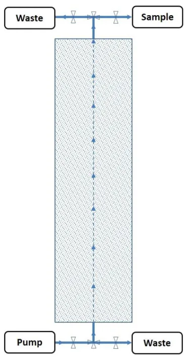
A vertical column porous medium system (Figure 1) was designed to pump fluid

through a porous media at the bottom of the column, and outflow samples were

collected at the top in a designed time sequence. The column was packed with 20/30

Accusand (Unimin Corporation, USA) with an air vibrator (Syntron, USA) to compress

the sand packing, and the diameter distribution and mean radius of the sand were

collected by laboratory colleagues Scott C. Hauswirth and Christopher A. Bowers [66],

whose paper is under review. The length and diameter of the column packed with

sand were measured and recorded, with density of the sand used to calculate the

porosity of the column porous medium. The inlet and outlet openings of the column

on both sides were closed with plugs with a middle hole to connect the inside and

outside of the domain system with plastic tubes. A syringe pump (Harvard Apparatus,

USA) was also connected to the column with plastic tubes and three-way and two-way

plastic valves to control the flow. CO2 (Industrial grade, Airgas) was injected into the

column for 30 minutes to push air bubbles out of the system completely, then

sufficient DIW was pumped with a constant flow rate into the system to saturate the

sand thoroughly and prepare the system for dispersion testing. Before every tracer

test, the inlet connection lines were cleaned and saturated with the same target fluids

(31)

20

Figure 1. Schematic of Column-Pump Porous Medium System

Guar Gum

Guar gum [67] is commonly and economically applied to produce non-Newtonian

fluids in hydraulic fracturing. Guar gum powder is produced from the endosperm of

seeds from the guar plant, also known as the cluster bean. Due to the physical

properties of guar gum as a galactomannan polysaccharide, dissolved guar gum

powder in water forms hydrogen bonds with water molecules and is broadly used as

(32)

21

used as a thickener and stabilizer in the petroleum and natural gas industries [68].

Guar gum powder was weighed and dissolved in DIW, DIW-tritium solution, along with

approximately 1 g sodium azide, diluted to 1 kg in total. The DIW-tritium solution was

further diluted about 100 times from the pre-diluted tritiated water based on the

purchased tritium. The mixture was then mixed at the highest speed in an electric

blender (Better Chef) for 30s and transferred into sealed glass containers after the

mixing was finished. Then the mixture was stirred slowly with a magnetic stir bar in a

magnetic stirrer (Thermix, Fisher Scientific) for about 24 hours until the guar gum was

fully dispersed. After that, the mixture was transferred into sealed plastic centrifuge

tubes and centrifuged for 30 minutes at 3100 R/min at 15℃ in a ventilated centrifuge (Marathon 21/R Ventilated Centrifuge, Fisher Scientific) to separate the potential

uneven insoluble ingredients of the mixture. After centrifugation, the upper solution

was homogenous and was collected as 0.05%, 0.1%, 0.2%, 0.3%, 0.4%, and 0.5% guar

gum solutions by mass, or guar gum tritium solutions if the DIW-tritium solution was

used to dissolve the guar gum powder. Before the solutions were injected into the

column, the DIW, DIW-tritium, guar gum, and guar gum tritium solutions were

degassed through a wall vacuum system in the laboratory to prevent air bubbles from

moving into the column system and maintain the saturated status of the domain.

Tracer Tests

Tracer tests were performed by observing the transport of tritium in either DIW or

guar gum solutions to quantify dilute species dispersion in both Newtonian and

non-Newtonian fluids. For the non-non-Newtonian fluids, the concentration of guar gum was

also a variable that was controlled. All experiments were run with a more viscous

(33)

22 displacement pattern.

DIW Up-Tracer Test: The plastic lines that connect the column with the pump were

cleaned and pre-saturated with a DIW-tritium solution. The DIW-tritium solution was

pumped at a flow rate (Q) of 40 mL/min (a velocity closes to general groundwater

velocity [69–71]) into the column pre-saturated with DIW starting at a certain time

(t=0) to replace DIW in the column. Outlet samples were then collected during the

whole tracer test from the top of the column into 20 mL disposable scintillation vials

(Fisher Scientific) at discrete and constant time intervals. The tracer concentration

exiting the column C=C(t) is referred to as a breakthrough curve. We assumed and

verified that after 1.6 pore volumes of the column of pumping the DIW-tritium

solution, the breakthrough curve reached steady-state, and we stopped the pump and

sample collecting. The steady-state concentration was verified by sequential sampling.

This experiment was designated the up-tracer test, as the radioactivity in the column

increases during the experimental period as a function of time.

DIW Down-Tracer Test: After the up-tracer test was completed; the column was

saturated with DIW-tritium solution. The syringe pump then was refilled with DIW,

and the plastic lines that connect the pump and the column were cleaned and

pre-saturated with DIW. We started the pump at a certain time (t=0) to inject DIW to

displace the DIW-tritium solution in the column, and we repeated the experimental

steps as in the up-tracer test in the same discrete and constant time intervals. This

experiment is called a down-tracer test because the radioactivity of the fluid in the

column is decreasing with time during the experiment. Both the up-tracer test and the

(34)

23

Guar Gum Tracer Test: For the guar gum tracer test, the column was first saturated

with DIW. The guar gum solutions of interest were at concentrations of 0.3%, and 0.5%

by mass. We picked these two specific concentrations of guar gum solution based on

some pre-research data from coworkers in the group in order to detect a clear

difference between Newtonian fluid and non-Newtonian fluid. When the

concentration of guar gum is small, the difference between the guar gum solution and

DIW is insignificant. In order to saturate the column with 0.3% guar gum solution, we

used a step-up saturating procedure, which means the column was saturated

step-by-step, first with 0.05%, then 0.1%, then 0.2%, and finally with 0.3% guar gum solution.

The purpose of the step-up saturating procedure was to minimize the potential

unstable flow inside the column system. After the column was saturated with 0.3%

guar gum, the same up-tracer test procedure was followed, in which a guar gum

tritium solution displaced a guar gum solution void of tritium, and outlet samples were

taken in the same time sequence as DIW tracer tests to track the relative radioactive

concentration in the output fluid. For the down-tracer guar gum tracer test, a guar

gum solution void of tritium displaced the resident guar gum-tritium solution, and the

same down-tracer samples were taken to observe the variation of the tracer in the

output fluid. Experiments were conducted with 0.3% and 0.5% guar gum solutions

separately, with the same step-up saturating procedure to saturate the column ahead

of the experiments.

Post-DIW tracer test: After the guar gum tracer experiments were performed, the

column was flushed with decreasing concentrations of guar gum solution void of

(35)

24

process. At least ten pore volumes of DIW were circulated to flush the guar gum from

the system before the post set of DIW tracer tests were performed. Following the

flushing procedure, the post-DIW tracer tests were performed with the same steps as

the DIW tracer test, and the same output samples were collected. The purpose of the

post-DIW tracer tests was to verify the column after conducting several guar gum

tracer tests.

Sample analysis: The samples collected from the tracer tests were combined with 8

mL liquid scintillation cocktail (Scintanalyzed, ScintiSafe Gel, Fisher Scientific, NC) and

1 mL of ethanol (200 proof, Decon Laboratories, Inc.) in sample vials. The liquid

scintillation cocktail was used to enhance the long-term stability of the samples,

improve counting efficiency, and reduce the contact time required for the

radioactivity detector during analysis [72–74]. The mixture was sealed and shaken by

hand immediately. The samples were then evaluated using a Tri-Carb 1900 TR Liquid

Scintillation Analyzer (Packard Instrument Co Inc, USA). Samples were analyzed in

triplicate, and the mean value of the three results for each sample were used for data

analysis. Tracer tests were repeated at least two times for each concentration of guar

gum solution, DIW tracer test, and post-DIW tracer test.

Simulations

Simulations consisted of four sections: the generation of media, the generation of

meshes, the simulation of the non-Newtonian fluid field, and the simulation of the

tracer transport in non-Newtonian fluid flowing through porous medium. The media

was generated by a specific sphere packing code [75] from former research group

(36)

25

conducted with OpenFOAM applications to generate the meshes and blocks for the

domain in order to obtain REV, simulate the saturating processes of the medium

domain with Newtonian fluid, and simulate the transport of dilute species in

non-Newtonian fluid passing through the pre-saturated domain system.

The first section allowed us to achieve domains with different sphere numbers and

target porosity. The second and third sections provided data to analyze and optimize

the better domain system and examine REV for the transport simulation. The last

section permitted us to observe the variation of the tracer transport in non-Newtonian

fluid passing through porous medium, obtaining microscale to macroscale data to

study the hydrodynamic dispersion of non-Newtonian fluids in a single fluid, porous

medium system. The outcome data were compared with the laboratory experimental

data to evaluate and verify the hydrodynamic dispersion of non-Newtonian fluids in

porous medium systems, as well as our research methods. The sphere packing code

ran at a local workstation, and OpenFOAM applications were executed in the

Dogwood cluster, a Linux-based computing system, at the University of North Carolina

at Chapel Hill.

Sphere Packing

To generate the media, sphere packing was used to pack the domain with randomly

generated hard spheres, with lognormal distribution of the size of spheres. The model

of packing impacts the porosity of the media and the distribution of the particles, as

well as the spheres, and therefore the behaviors of fluids and the domain system. This

work applied Sphere Packing code from our group members [75,76] for random

packing of incompressible spheres, with number of spheres Ns set as 1000, 2000, 3000,

(37)

26

The initial porosity was 0.8, and target porosity was 0.36; the lengths of the domain in

each of three-dimensions were the same for any one of the sphere domains and were

specified by the expected volume of the lognormal packing as shown in Eq. (3). The

lognormal distribution variance σ2_{was 0.004318914893.}

4𝜋𝑁𝑠

3 𝐸[𝑟

3_{] =}4𝜋𝑁𝑠

3 exp (3𝜇𝑙𝑜𝑔+ 9 2𝜎

2_); ₍₃₎

where 𝜇𝑙𝑜𝑔 is the lognormal mean and 𝑟 is the radius of sphere [L]. Since it is not

possible to specify 𝜇_𝑙𝑜𝑔, 𝜎2_{, and porosity}_{ε indepen}_{dently, we specified certain}_𝜎2_and

the target porosity, after which the value 𝜇𝑙𝑜𝑔 can be approximated based on these

two data. The mean diameter of the spheres was the same as the mean diameter of

sand used for the laboratory column-pump system; the mean radius of the spheres

can be calculated by Eq. (4):

𝑟̅ = exp [𝜇_𝑙𝑜𝑔+𝜎

2

2]; (4)

The generated domain systems were applied in the OpenFOAM simulations described

below.

OpenFOAM Simulation

The Open Source Field Operation and Manipulation (OpenFOAM), a popular

open-source mathematical methods C++ library, was introduced to conduct computation

for dilute species dispersion of Non-Newtonian fluids in the Linux-based system. Here

we used the OpenFOAM User Guide (Version 6) [77] from the OpenFOAM source

website to guide the simulation processes and ParaView to visualize and analyze some

of the results of the simulation.

(38)

27

The pre-processing was the application of a specific mesh generator in OpenFOAM,

snappyHexMesh, to create hexahedra (hex) and split-hexahedra (split-hex) for the

three-dimensional meshes in Stereolithography (STL) or tri-surfaces. By iteratively

refining the existing meshes generated through blockMesh and morphing the refined

meshes to the surfaces of STL, snappyHexMesh created fine meshes with variable

refinement levels to fit onto a given geometry. In general, the higher the refinement

level, the more accurate the generated mesh will be, but the calculation processes for

the computer to solve will be significantly larger and time-consuming. The

snappyHexMeshDict dictionary provided a place to adjust the parameters of

snappyHexMesh.

Under system directory, the application blockMesh was applied to generate blocks in

three-dimensions on an x-y-z plane. The boundaries and initial conditions and other

fields can be set up through different system data files. DecomposeParDict decided

the number of decomposed blocks of the domain. ControlDict was responsible for

control of time, such as the beginning and end of run time, time interval, and reading

and editing field data. decomposePar was the application used for parallel processing

in research computing, followed by reconstructPar to reconstruct the mesh fields.

blockMesh builds the mesh with blocks, and the different blocks number will impact

the accuracy of the approximate solution for the partial differential algebraic

equations (PDAE) and calculation counts. Eventually, the sphere domains with

different sphere numbers were refined to 1003_{(x-y-z as: 120}_×₁₀₀_×_{100, same}

sequence for following blocks), 2003₍₂₄₀_×₂₀₀_×_{200), and 300}3₍₃₆₀_×₃₀₀_×₃₀₀₎

(39)

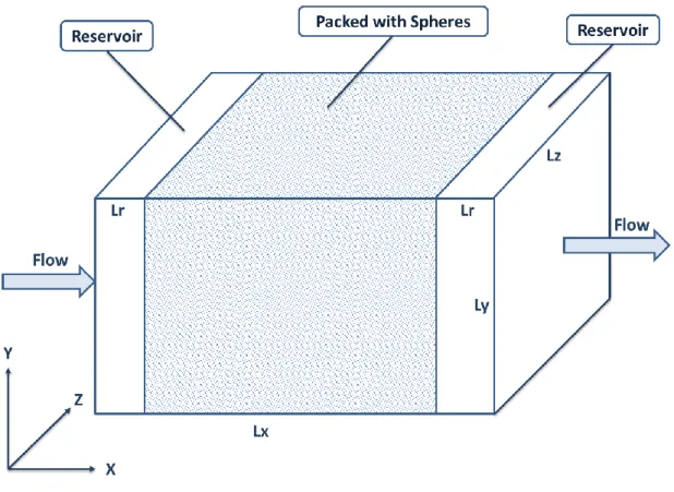
28

(600×500×500) blocks for selected domains. The difference in the x-axis is because the domains were rectangular, and because of the two reservoirs in two sides of the

domain, the inlet and outlet, which were used to make sure the flow had the same

velocity and direction when it encountered the sphere domains. The schematic of the

domain system is shown in Figure 2.

Figure 2. Schematic of Domain System

The lengths of the entire domain follow Eq. (5), and 𝐿₀ is the packed domain length derived from Sphere Packing; 𝐿_𝑟 is the length of the reservoir. The packed area of the entire domain is a cube, but because of the existence of the two reservoirs, the entire

domain is a cuboid.

𝐿_𝑥 = 1.2𝐿_𝑦 = 1.2𝐿_𝑧; 𝐿_𝑦 = 𝐿_𝑧= 𝐿₀; 𝐿_𝑟 = 0.1𝐿₀; ₍₅₎

Because of the reservoirs, the actual porosity of the domain was not the same as the

(40)

29

system was collected by checkMesh, and was used to calculate the actual porosity of

the entire domain system.

Non-Newtonian fluid field

After the execution of snappyHexMesh, the next step was nonNewtonianIcoFoam and

the following post-processing. The nonNewtonianIcoFoam solver was used to solve

the incompressible laminar flow movement for non-Newtonian fluids. For IcoFoam

[78], it is a specific numerical method code that was designed to solve incompressible

laminar Navier-Stokes equations [79–81] for viscous fluids by using Pressure-Implicit

with Splitting of Operators (PISO) algorithm [82,83]. Navier-Stokes equations are a

continuum with a set of partial differential equations derived from the momentum

conservation equation for the viscous fluid system at the scale of interest (microscale

here) by applying Newton’s second law as a closure relation. Navier-Stokes equations

include the pressure term and the stress applied on the fluid to simulate the unstable

viscosity of the non-Newtonian fluid’s movement specifically, and they have been

widely applied in fluid mechanics, engineering, and other fluid scientific areas. PISO is

an improved algorithm based on the SIMPLE algorithm by Issa [84] to calculate

pressure-velocity for Navier-Stokes equations with larger time steps and accordingly

less computational effort. The incompressible Navier-Stokes equation is as follows Eq.

(6) [85]:

𝜕𝒖

𝜕𝑡 + (𝒖 ∙ 𝜵)𝒖 − ν𝜵

2_{𝒖 = −𝜵𝜔 + 𝑔;} ₍₆₎

(41)

30

mass; and 𝑔 is the gravity acceleration [L/T2_];_𝛻𝜔_{is estimated by Eq. (7):}

𝜵𝜔 ≡ 1

𝜌₀𝜵𝑝 = 𝜵( 𝑃

𝜌₀); (7)

where 𝜌₀ is the uniform density of the fluid for incompressible fluid (here we assume the density variation is negligible); and 𝑝 is the pressure [M/LT2_{]. The}_{Stokes’s stress}

constitutive equation for incompressible viscous flow is Eq. (8):

𝝉 = 𝜇(𝜵𝒖 + 𝜵𝒖𝑻); ₍₈₎

where 𝝉represents the shear stress tensor [M/LT2_{]; and}_𝜇_is_{dynamic viscosity}_[M/LT].

The relationship between kinematic viscosity and dynamic viscosity can be formulated

as Eq. (9):

ν =𝜇

𝜌; (9)

Substituting Eq. (7-9) into Eq. (6), the partial differential equations can be solvable

with boundary conditions. To solve these complicated partial differential equations

with respect to three-dimensions and time, we usually apply numerical methods to

solve for the approximate solution within acceptable error. Navier-Stokes first can be

discretized by the finite volume method, then in each time step, the PISO algorithm

[82] takes the discretized equations with initial predict and boundary conditions to

compute the velocity field and mass fluxes at the blocks faces from the

snappyHexMesh step, and solve for pressure in blocks in the domain. Then mass fluxes

and velocities are corrected based on the newly solved pressure field, and the

boundary conditions are updated. These steps are repeated until the computational

error is smaller than the acceptable error to convergence. After the iterations in one

(42)

31

time step reaches the set end time. The PISO algorithm is suitable for resolving

velocity-pressure problems.

In the first set of nonNewtonianIcoFoam simulations, we tested each domain system

from the snappyHexMesh step with a constant velocity

(𝑣 = 0.00005 𝑚/𝑠) (a velocity closes to the velocity used in experimental tracer tests and the general groundwater velocity) and the viscosity data for 0.3% guar gum

solution by mass, collected pressure drop data for each domain system, and analyzed

the data. This allowed us to evaluate REV based on the conductivity of the domain

system, and to select the appropriate domain system for the transport simulations.

Specifically, we took the polyMesh solution data from snappyHexMesh for each sphere

packing domain to the non-Newtonian solver and solved for pressure drop data with

given boundary conditions. After running the same decomposePar to decompose the

meshes, nonNewtonianIcoFoam was run in parallel to solve the non-Newtonian fluids

passing through the porous medium, and reconstructPar for reconstruction in time

sequence. The post-processing uses patchAverage, which solves for pressure drop for

the whole domain at different time stamps. The variation of the pressure drop on the

whole domain with respect to time can be evaluated if the domain system is

steady-state. This step is the counterpart of the saturation process in the laboratory tracer

tests.

A difference in controlDic is that courant number 𝛼 must be smaller than 1 according to the following Eq. (10) [77]:

𝛼 =𝛿𝑡

(43)

32

in which 𝛿𝑡 represents deltaT, 𝛿𝑥 is the size of the cell, and |𝑣| is the velocity. Based on this equation, 𝛼 can be adjusted by manipulating 𝛿𝑡 and 𝛿𝑥 to make sure it obeys the rule. The courant number also can be found from the nonNewtonianIcoFoam

output log to examine any error and adjust the setting accordingly.

Other dictionaries, like fvSchemes and fvSolution dictionaries in system directory,

were not needed to edit or change any parameter, and therefore are not discussed.

Physical properties, such as Reynolds number and velocity, were assigned by

transportProperties dictionary.

In the second set of nonNewtonianIcoFoam simulations, we took the selected domain

system, then assigned different velocities (𝑣 = 0.0005 𝑚/𝑠; 0.00005 𝑚/

𝑠; 0.000005 𝑚/𝑠) respectively to three viscosity data: DIW, 0.3% and 0.5% guar gum by mass solutions separately on the domain system. We then ran

nonNewtonianIcoFoam again to acquire velocity data for the saturated steady-state

domain systems for the following transport simulation. The rheological measurements

of the three viscosity data were investigated by laboratory colleague P.B. Schultz who

applied a stress-controlled rheometer with a temperature-controlled plate and

Rheology Advantage Instrument Control software program to analyze the

measurements of viscosity at different shear rates for every guar gum sample. The

cross-power law model used for kinematic viscosity for non-Newtonian fluids in

OpenFOAM computing is Eq. (11):

ν = ν_∞+ (ν0− ν∞)

1 + (𝑚𝛾̇)𝑛; (11)

(44)

33

respectively; 𝑚 and 𝑛 are two fitting parameters; and 𝛾̇ is the shear rate.

ParaView was ultilized to visualize the domain system. Because the system is too large

for the local workstation to do the processes for ParaView, ParaView was executed in

the Longleaf cluster [86], another Linux-based computing system at the University of

North Carolina at Chapel Hill, used particularly for a single compute host that requires

large workloads.

Species Transport

The scalarTransportFoam application [87] from OpenFOAM was used to solve species

transport equations for the concentration data with the specified velocity field data

from nonNewtonianIcoFoam. scalarTransportFoam typically evaluates the

approximate solutions for scalar convection-diffusion problems under certain

boundary conditions. Here the boundary conditions are the fixed value of

concentrations of species at the inlet (𝑇0 = 1) and zero gradient at the outlet of the

domain system. The convection-diffusion equation solved by the

scalarTransportFoam application is Eq. (12):

𝜕𝑇

𝜕𝐿+ 𝛁 ∙ (𝑼𝑇) − 𝛁

2_(𝐷

𝑇𝑇) = 0; (12)

in which 𝑇 represents the transported scalar with zero order, here the relative

concentration of the species 𝐶

𝐶0; 𝑼is the velocity vector of the fluid; and 𝐷𝑇 is the

molecular diffusion coefficient divided by the density of the fluid. In

scalarTransportFoam solver, the molecular diffusion coefficient and the fluid density

are assumed as constants. Since the longitudinal direction is the direction of interest,

(45)

34

resolve approximate solutions for the transient transport equations is the finite

volume method, the same as nonNewtonianIcoFoam.

The selected domains were applied in scalarTransportFoam after solved by

nonNewtonianIcoFoam with different velocities and concentrations of the guar gum

solutions. The velocity vector data was specified to the scalarTransport directory,

along with the polyMesh data. We assigned the 𝐷𝑇 = 2.05𝐸 − 10 according to two studies [88,89] in transportProperties dictionary, and set another 𝐷_𝑇 = 0 as a comparison.

Each of the entire domains was decomposed to a certain number of small domains,

then the transport of species was computed in parallel at a certain time interval in the

Dogwood cluster, and the transient relative concentration and time stamp were

calculated and recorded by reconstrucPar and postProcessing applications. The

relative concentration variations with respect to time were collected for the following

analysis. The same system directory was used to adjust parameters for the simulation

to run efficiently and appropriately.

Dogwood and Longleaf Clusters

The Dogwood cluster and Longleaf cluster [90] at the University of North Carolina at

Chapel Hill are both Linux-based scientific computing systems that are available for

students, faculties, and other researchers around campus to use for free. The

Dogwood cluster has over 11,000 computing cores, large scratch disk space, and

high-speed bandwidth to provide outstanding computing equipment for large, parallel MPI,

or hybrid scientific programming models. The cluster uses Intel Xeon Skylake and Phi