E
SSAYS ONC
ONDITIONALQ
UANTILEE
STIMATION ANDE
QUITYM
ARKETD
OWNSIDER
ISKHanwei Liu
A dissertation submitted to the faculty of the University of North Carolina at Chapel Hill in par-tial fulfillment of the requirements for the degree of Doctor of Philosophy in the Department of
Economics.
Chapel Hill 2017
Approved by:
Eric Ghysels
Peter Hansen
Jonathan Hill
Chuanshu Ji
c
2017
Hanwei Liu
ABSTRACT
HANWEI LIU: Essays on Conditional Quantile Estimation and Equity Market Downside Risk. (Under the direction of Eric Ghysels)
Fully aware of the importance of effective risk management, we develop the HYBRID-quantile
model aimed at enhancing the accuracy of conditional quantile predictions. In the first essay, we
validate that the model has a strong performance when applied to various GARCH-type processes.
We use conditional asymmetry measures derived from the conditional quantile predictions to
de-sign portfolio allocation strategies. We identify two portfolios that could improve upon the
risk-return trade-off of the benchmarks.
In the second essay, we study the downside risk in the Chinese equity market. A wide range
of investors, both domestic and foreign, have paid more attention to the Chinese stock market
because of the growing significance of the Chinese economy. Downside risk has been a focal
point, particularly considering the large price movements and the regulatory changes that took
place over time. We use the 1% and 5% conditional quantiles of equity index returns to study
the pattern of downside risk, and discover several break dates linked to major financial crises
and trading reforms. Furthermore, our findings indicate that breaks in the B shares and the H
shares downside risk tend to appear earlier than those corresponding to the A shares tails. Lastly,
the revised Qualified Foreign Institutional Investor (QFII) program in 2006 and government share
purchasing actions in 2015 have shown to be effective at alleviating downside risks in the Shanghai
A shares.
In the third essay, a joint work with Eric Ghysels and Steve Raymond, we examine granularity
in the U.S. stock market. The U.S. equities market price process is largely driven by large
insti-tutional investors. We use quarterly 13-F holdings reported by instiinsti-tutional investors and focus on
the Herfindahl-Hirschman Index (HHI) as the measure of granularity. We provide a
across stocks and (3) downside risk. We find that constructing a low-HHI minus high-HHI
portfo-lio produces an annualized return of 5.6%, and a 6.2% liquidity risk-adjusted return. We document
the adverse impact that investor ownership concentration has on both conditional volatility, and
ACKNOWLEDGMENTS
This long and winding journey of Ph.D. is not an easy feat and by no means a solo effort.
I would like to first express the deepest gratitude to my advisor, Prof. Eric Ghysels, who
pro-vided guidance and insights that have been instrumental to the development of my dissertation and
perpetually inspires me through his enthusiasm in research. I am also grateful to my committee
members for their constructive feedback and encouragements that helped immensely in
advanc-ing my work. I would like to thank all participants at the UNC Econometrics workshop for their
efforts put into the presentations and discussions. In particular, I wish to convey my utmost
appre-ciation to Steve Raymond for his exceptional commitment to our joint project and for being the
best collaborator one could ask for.
On a personal front, I would like to give a heartfelt thank you to some of my closest friends (C,
Q, Yiyi, Teresa, and Herbie, to name a few). Your solidarity without a doubt became indispensable
to me during cheerful and dismal times alike, and I wish you the best of luck in all your endeavors.
Finally, to my dearest and greatest parents, Xinli Liu and Xingping Wang, who first brought me
to the fascinating realm of Economics and have shown me nothing but unwavering support ever
since. Your unconditional love carried me through the ebbs and flows, transcended the time
dif-ference and the vast space between us, and made it considerably easier to overcome the seemingly
insurmountable solitude in this odyssey. It fills me with pride and joy to say that this is for you,
TABLE OF CONTENTS
LIST OF TABLES . . . x
LIST OF FIGURES . . . xvi
1 Stock Return Quantiles and Conditional Asymmetry . . . 1
1.1 Introduction . . . 1
1.2 Quantile Estimation Models . . . 2
1.2.1 CAViaR Model . . . 3
1.2.2 MIDAS Model . . . 4
1.2.3 HYBRID Model . . . 5
1.3 Model Evaluation . . . 7
1.3.1 Hit Statistic and Dynamic Quantile Test . . . 7
1.3.2 Kupiec Tests . . . 8
1.3.3 Christoffersen test . . . 9
1.3.4 Bootstrapping Empirical Quantiles from GARCH-type DGPs . . . 10
1.4 Empirical Results . . . 13
1.4.1 Stock Return Series Summary Statistics . . . 13
1.4.2 Parameter Estimates and Test Statistics . . . 15
1.4.3 Benchmark Quantiles from GARCH-based Parametric Bootstrapping . . . 19
1.4.4 The Financial Crisis of 2008: An Event Study . . . 22
1.4.5 Conditional Asymmetry . . . 27
1.6 Concluding Remarks . . . 31
2 Has the Downside Risk in the Chinese Stock Market Fundamentally Changed? . . . 32
2.1 Introduction . . . 32
2.2 An Overview of the Chinese Equity Market . . . 33
2.2.1 Data . . . 35
2.2.2 Prior literature . . . 38
2.3 Model Specifications and Tests . . . 41
2.3.1 Conditional Quantile Estimation . . . 41
2.3.2 Backtesting and Breaks Detection . . . 43
2.4 Empirical Results . . . 44
2.4.1 Parameter Estimates and Conditional Quantile Predictions . . . 44
2.4.2 Bivariate Estimates . . . 45
2.4.3 Break Points Identified in the Downside Risks . . . 49
2.4.4 Break Points Revisited . . . 55
2.5 Assessing Government Measures . . . 57
2.5.1 The QFII Program . . . 57
2.5.2 Year in Focus - The Chinese Stock Market Turbulence . . . 58
2.6 Concluding Remarks . . . 60
3 Granularity and (Downside) Risk in Equity Markets . . . 61
3.1 Introduction . . . 61
3.2 Expected Returns, Volatility and Downside Risk . . . 63
3.2.1 Conditional Means – Linear Factor Models . . . 67
3.2.2 Conditional Volatility . . . 68
3.2.3 Downside Risk . . . 73
3.3.1 Portfolio-Level Downside Risk by Top Players . . . 76
3.3.2 Firm-Level Downside Risk by Top Players . . . 83
3.3.3 Evidence from options markets . . . 84
3.4 Reduced Form Model . . . 86
3.5 Conclusion . . . 90
A Appendix A: Conditional Quantile . . . 91
A.1 Coefficient Estimates and Backtesting Results . . . 91
A.2 Conditional Quantile Plots . . . 103
A.3 Unconditional Quantiles . . . 109
A.4 Conditional Quantile Forecasts Loss Values . . . 111
A.5 Conditional Asymmetry Plots . . . 168
B Appendix B: Downside Risk in Chinese Market . . . 172
B.1 Conditional Quantile Estimation . . . 172
B.2 Backtests . . . 175
B.3 Structural Break Tests . . . 177
B.3.1 Testing Parameter Constancy . . . 177
B.3.2 Multiple Breaks Tests . . . 179
B.3.3 Structural Changes in Regression Quantiles . . . 180
B.4 Parameter Estimates and Break Tests Results . . . 182
C Appendix C: Granularity . . . 204
C.1 HHI Portfolio Analysis Details . . . 204
C.1.1 Portfolio Construction . . . 204
C.1.2 HHI Decomposition . . . 206
C.1.3 Low-Minus-High (LMH) Portfolio Characteristics . . . 206
C.2.1 Downside Risk . . . 208
C.2.2 Downside Risk with Decomposed HHI . . . 209
C.3 Reduced Form Model Details . . . 213
LIST OF TABLES
1.1 Market Indices Summary Statistics: Jan. 3, 2000 - Oct. 30, 2015 . . . 14
1.2 Market Indices Summary Statistics: Jan. 3, 2000 - Oct. 30, 2015 . . . 15
1.3 Conditional Quantile Coefficient Estimates - S&P 500 . . . 16
1.4 Backtests - S&P 500 . . . 17
1.5 Backtests - MIDAS vs. U-MIDAS Weights . . . 19
1.6 Unconditional Quantiles from GARCH Parametric Bootstrapping - S&P 500 . . . . 21
1.7 US - MSE . . . 23
1.8 US - Exponential Bregman, a = 1 . . . 24
1.9 Crisis Period Parameter Estimates - S&P 500 . . . 25
1.10 Crisis Period Backtests - S&P 500 . . . 26
1.11 Asset Allocation Summary . . . 29
1.12 Portfolio Risk-Return Profile . . . 30
2.1 Market Overview - Shanghai & Shenzhen Stock Exchange Dec. 2016 . . . 34
2.2 Summary Statistics Daily Returns . . . 36
2.3 Major Events in the Chinese Stock Market . . . 39
2.4 HYBRID-SAV Conditional Quantile Parameter Estimates . . . 44
2.5 DQ, Kupiec, and Christoffersen Tests . . . 46
2.6 HYBRID-SAV Conditional Quantile Bivariate Parameter Estimates . . . 47
2.7 HYBRID-SAV Break Dates . . . 50
2.8 Structural Changes Test Statistics - A, B and H Shares . . . 52
2.9 Break Dates - Volume + Lending Rate . . . 55
2.10 Structural Change Test - A/B/H Share + Volume + Lending Rate . . . 56
3.1 Annualized HHI Low-High Portfolio Returns . . . 67
3.2 Linear Factor Correlations . . . 67
3.3 Conditional Mean Linear Factor Models . . . 69
3.4 Conditional Volatility Regressions – Quarterly . . . 70
3.5 Conditional Volatility Regressions – Monthly . . . 71
3.6 Regression of Conditional Quantile on HHI . . . 75
3.7 Top Institutions Holding Decomposition . . . 77
3.8 Regression of Conditional Quantile on Decomposed HHI . . . 79
3.9 Regression of Conditional Quantile on HHI - Quarterly . . . 80
3.10 Regression of Conditional Quantile on Decomposed HHI - Quarterly . . . 81
3.11 Regression of Conditional Quantile on HHI - First Month . . . 83
3.12 Firm-Level Risk on Investor Concentration Regressions . . . 85
3.13 HHI-Factor Linear Asset Pricing Model . . . 89
3.14 Regression of Conditional Quantile on HHI: Simulated Data . . . 90
A.1 Conditional Quantile Coefficient Estimates - S&P 500 . . . 91
A.2 Conditional Quantile Coefficient Estimates - FTSE 100 . . . 92
A.3 Conditional Quantile Coefficient Estimates - STOXX 50 . . . 93
A.4 Conditional Quantile Coefficient Estimates - Nikkei 225 . . . 94
A.5 Conditional Quantile Coefficient Estimates - SSE . . . 95
A.6 Conditional Quantile Coefficient Estimates - IPC . . . 96
A.7 Conditional Quantile Coefficient Estimates - ASX . . . 97
A.8 Conditional Quantile Coefficient Estimates - Bovespa . . . 98
A.9 Conditional Quantile Coefficient Estimates - TSX . . . 99
A.10 Conditional Quantile Coefficient Estimates - DAX . . . 100
A.12 Conditional Quantile Coefficient Estimates - HSI . . . 102
A.13 1%, 2.5%, and 5% Unconditional Quantiles - UK, EU, Japan, and China . . . 109
A.14 1%, 2.5%, and 5% Unconditional Quantiles - Mexico, Australia, and Brazil . . . . 109
A.15 1%, 2.5%, and 5% Unconditional Quantiles - Canada, Germany, France, and HK . 110 A.16 US - MSE, GARCH + EGARCH . . . 111
A.17 US - MSE, GJR-GARCH + IGARCH + TGARCH . . . 112
A.18 US - MAE, GARCH + EGARCH . . . 113
A.19 US - MAE, GJR-GARCH + IGARCH + TGARCH . . . 114
A.20 US - Exponential Bregman, a = 1, GARCH + EGARCH . . . 115
A.21 US - Exponential Bregman, a = 1, GJR-GARCH + IGARCH + TGARCH . . . 116
A.22 UK - MSE, GARCH + EGARCH . . . 117
A.23 UK - MSE, GJR-GARCH + IGARCH + TGARCH . . . 118
A.24 UK - MAE, GARCH + EGARCH . . . 119
A.25 UK - MAE, GJR-GARCH + IGARCH + TGARCH . . . 120
A.26 UK - Exponential Bregman, a = 1, GARCH + EGARCH . . . 121
A.27 UK - Exponential Bregman, a = 1, GJR-GARCH + IGARCH + TGARCH . . . 122
A.28 EU - MSE . . . 123
A.29 EU - MAE . . . 124
A.30 EU - Exponential Bregman, a = 1 . . . 125
A.31 Japan - MSE . . . 126
A.32 Japan - MAE . . . 127
A.33 Japan - Exponential Bregman, a = 1 . . . 128
A.34 China - MSE, GARCH + EGARCH . . . 129
A.35 China - MSE, GJR-GARCH + IGARCH + TGARCH . . . 130
A.37 China - MAE, GJR-GARCH + IGARCH + TGARCH . . . 132
A.38 China - Exponential Bregman, a = 1, GARCH + EGARCH . . . 133
A.39 China - Exponential Bregman, a = 1, GJR-GARCH + IGARCH + TGARCH . . . . 134
A.40 Mexico - MSE . . . 135
A.41 Mexico - MAE . . . 136
A.42 Mexico - Exponential Bregman, a = 1 . . . 137
A.43 Australia - MSE, GARCH + EGARCH . . . 138
A.44 Australia - MSE, GJR-GARCH + IGARCH + TGARCH . . . 139
A.45 Australia - MAE, GARCH + EGARCH . . . 140
A.46 Australia - MAE, GJR-GARCH + IGARCH + TGARCH . . . 141
A.47 Australia - Exponential Bregman, a = 1, GARCH + EGARCH . . . 142
A.48 Australia - Exponential Bregman, a = 1, GJR-GARCH + IGARCH + TGARCH . . 143
A.49 Brazil - MSE, GARCH + EGARCH . . . 144
A.50 Brazil - MSE, GJR-GARCH + IGARCH + TGARCH . . . 145
A.51 Brazil - MAE, GARCH + EGARCH . . . 146
A.52 Brazil - MAE, GJR-GARCH + IGARCH + TGARCH . . . 147
A.53 Brazil - Exponential Bregman, a = 1, GARCH + EGARCH . . . 148
A.54 Brazil - Exponential Bregman, a = 1, GJR-GARCH + IGARCH + TGARCH . . . . 149
A.55 Canada - MSE, GARCH + EGARCH . . . 150
A.56 Canada - MSE, GJR-GARCH + IGARCH + TGARCH . . . 151
A.57 Canada - MAE, GARCH + EGARCH . . . 152
A.58 Canada - MAE, GJR-GARCH + IGARCH + TGARCH . . . 153
A.59 Canada - Exponential Bregman, a = 1, GARCH + EGARCH . . . 154
A.60 Canada - Exponential Bregman, a = 1, GJR-GARCH + IGARCH + TGARCH . . . 155
A.62 Germany - MAE . . . 157
A.63 Germany - Exponential Bregman, a = 1 . . . 158
A.64 France - MSE . . . 159
A.65 France - MAE . . . 160
A.66 France - Exponential Bregman, a = 1 . . . 161
A.67 Hong Kong - MSE, GARCH + EGARCH . . . 162
A.68 Hong Kong - MSE, GJR-GARCH + IGARCH + TGARCH . . . 163
A.69 Hong Kong - MAE, GARCH + EGARCH . . . 164
A.70 Hong Kong - MAE, GJR-GARCH + IGARCH + TGARCH . . . 165
A.71 Hong Kong - Exponential Bregman, a = 1, GARCH + EGARCH . . . 166
A.72 Hong Kong - Exponential Bregman, a = 1, GJR-GARCH + IGARCH + TGARCH . 167 B.1 MIDAS-SAV Conditional Quantile Parameter Estimates . . . 182
B.2 CAViaR-SAV Conditional Quantile Parameter Estimates . . . 182
B.3 HYBRID-AS Conditional Quantile Parameter Estimates . . . 183
B.4 MIDAS-AS Conditional Quantile Parameter Estimates . . . 184
B.5 CAViaR-AS Conditional Quantile Parameter Estimates . . . 184
B.6 DQ, Kupiec & Christoffersen Test Statistics - Shanghai A Share Index . . . 185
B.7 DQ, Kupiec & Christoffersen Test Statistics - Shanghai B Share Index . . . 186
B.8 DQ, Kupiec & Christoffersen Test Statistics - H Share Index . . . 187
B.9 HYBRID-AS Break Dates . . . 188
B.10 Structural Changes Test Statistics - A, B and H Shares . . . 189
B.11 Conditional Quantile Coefficient Estimates - Volume . . . 190
B.12 Conditional Quantile Coefficient Estimates - Volume and Lending Rate . . . 191
B.13 QFII Program Subsamples - Shanghai A Shares, MIDAS-SAV model . . . 192
B.15 QFII Program Subsamples - Shanghai A Shares, HYBRID-AS model . . . 193
B.16 QFII Program Subsamples - Shanghai A Shares, MIDAS-AS model . . . 194
B.17 QFII Program Subsamples - Shanghai A Shares, CAViaR-AS model . . . 195
C.1 Portfolio HHI Summary Statistics . . . 205
C.2 Portfolio HHI Decomposition . . . 206
C.3 Annualized Portfolio Returns . . . 207
C.4 Liquidity-Risk Adjusted Excess Returns . . . 207
C.5 Regression of Conditional Quantile on HHI: Pre-crisis . . . 208
C.6 Regression of Conditional Quantile on Quarterly HHI - Pre-crisis . . . 209
C.7 Regression of Conditional Quantile on Decomposed HHI - Pre-crisis . . . 210
C.8 Regression of Conditional Quantile on Quarterly Decomposed HHI - Pre-crisis . . 211
C.9 Regression of Conditional Quantile on HHI - First Month Pre-crisis . . . 212
LIST OF FIGURES
1.1 Homogeneous Bregman and Exponential Bregman functions . . . 12
1.2 5% Conditional Quantile - US . . . 20
1.3 Conditional Asymmetry - US . . . 27
3.1 Quarterly Top Institutional Investor Market Shares . . . 65
3.2 Quarterly HHI . . . 66
3.3 Conditional Volatility High versus Low HHI Portfolio . . . 73
3.4 Conditional Quantile Estimates HHI Portfolios 5% Left Tail . . . 74
A.1 Conditional Quantiles - US . . . 103
A.2 Conditional Quantiles - UK . . . 103
A.3 Conditional Quantiles - EU . . . 104
A.4 Conditional Quantiles - Japan . . . 104
A.5 Conditional Quantiles - China . . . 105
A.6 Conditional Quantiles - Mexico . . . 105
A.7 Conditional Quantiles - Australia . . . 106
A.8 Conditional Quantiles - Brazil . . . 106
A.9 Conditional Quantiles - Canada . . . 107
A.10 Conditional Quantiles - Germany . . . 107
A.11 Conditional Quantiles - France . . . 108
A.12 Conditional Quantiles - Hong Kong . . . 108
A.13 Conditional Asymmetry - US . . . 168
A.14 Conditional Asymmetry - UK . . . 168
A.15 Conditional Asymmetry - EU . . . 169
A.17 Conditional Asymmetry - Brazil . . . 170
A.18 Conditional Asymmetry - Canada . . . 170
A.19 Conditional Asymmetry - France . . . 171
A.20 Conditional Asymmetry - Hong Kong . . . 171
B.1 Shanghai Stock Exchange Composite Index Daily Returns . . . 196
B.2 Shanghai Stock Exchange Monthly Trading Volume - Trillions . . . 196
B.3 Shenzhen Stock Exchange Component Index Daily Returns . . . 197
B.4 H-Share Index Daily Returns . . . 197
B.5 1% and 5% Tail Breaks - Shanghai A & Shanghai B . . . 198
B.6 1% and 5% Tail Breaks - Shanghai A & Hong Kong . . . 199
B.7 Lending Rate - Mainland China & Hong Kong . . . 200
B.8 Shanghai A-Share Index 1% and 5% Tails - Jan. 2015 to Dec. 2016 . . . 201
B.9 Shanghai A-Share Index 1% and 5% Tails - Post-Intervention . . . 202
B.10 Shanghai A-Share Index, Full vs. Post-Intervention Sample . . . 203
C.1 Quarterly Number of Institutional Investors . . . 204
1 Stock Return Quantiles and Conditional Asymmetry - An Approach to Portfolio Selection
1.1 Introduction
The financial industry has been placing an increasing emphasis on effective risk management.
This is an essential part of any adequate investment strategy, especially after the grim reality of
the financial crisis. One of the commonly cited measures is value at risk (VaR), which represents
the maximum amount a portfolio can lose within a certain time frame given a confidence level.
Instead of a monetary amount, we can also transform the measure into a proportion of the total
amount invested. From this perspective, we are examining the quantiles of future portfolio returns.
Specific to this purpose, we would like to form forecasts of the return quantiles and improve upon
existing models in the literature. Negative skewness, excess kurtosis, and extreme realizations of
financial returns all pose a challenge to using conditional volatility as the only measure of downside
risk, and point to utilizing conditional quantile of the return distribution. Another challenge is that
quantile regressions under the GARCH framework are relatively cumbersome. We therefore seek
other resolutions to the issue at hand.
Our estimation process follows the dynamic additive quantile literature (Koenker and Xiao
(2006), Gourieroux and Jasiak (2008)) and the mixed-frequency data literature Ghysels,
Santa-Clara, and Valkanov (2006), in that our model consists of an autoregressive and a mixed-frequency
component. An equally important stream of reference includes the conditional autoregressive
value-at-risk model (Engle and Manganelli (2004)) and its extension to the multivariate and
multi-quantile arena (White, Kim, and Manganelli (2015)). Assuming the standpoint of an international
investor, we explore the effect of exposure in developed markets as well as emerging markets. This
is also elaborated in the conditional skewness literature (Ghysels, Plazzi, and Valkanov (2016)).
We propose the HYBRID-quantile model to predict weekly conditional quantiles of several
Ghysels, and Wang (2015) and a direct application to conditional quantile estimations. Daily return
information is captured by a mixed-frequency term that projects the returns onto a weekly horizon.
We review the outputs for the 1%, 2.5%, and 5% conditiona quantiles. Taking a more prudent
approach, we lean towards allowing higher possible losses when discrepancies with true return
quantiles exist. Namely, we would rather underestimate the lower tails of index returns so as to
better prepare for large unexpected drops in portfolio values. This characteristic will be reflected
in the loss function of our choice.
The paper is organized as follows. Section 1.2 introduces the HYBRID quantile forecasting
model and reviews the other two candidates, CAViaR and MIDAS model. Section 1.3 lists the
backtests, a simulation procedure we adopted to extract the benchmark population quantiles, and
the asymmetric loss functions we took to evaluate the forecasts. Section 1.4 describes the data
sample, summarizes the empirical results, and includes an exercise focusing on the crisis period.
Section 1.5 discusses potential portfolio allocation strategies and their risk-return indications.
Sec-tion 1.6 concludes the analyses.
1.2 Quantile Estimation Models
In this section, we review the two benchmark models that we examined in the quantile
fore-casting process. We subsequently introduce the model of interest in this paper, a model with a
HYBRID data structure. All three models entail modeling a number of chosen quantiles directly
instead of modeling the entire return distribution.
Assume that we obtain a vector of portfolio returns,{rt}Tt=1. As is typical in the literature, all
of the returns referred to in this paper are log returns to allow temporal aggregation. The n-period
log return is defined as
rt,n= n−1
X
j=0
rt+j. (1.2.1)
We denote the probability associated with a target VaR asθ, i.e.:
and the parameter estimatesβˆare set up to solve
min
β
1
T T
X
t=1
[θ−I(rt,n < qt,n(β;θ))][rt,n−qt,n(β;θ)]. (1.2.3)
The indicator functionI(rt,n < qt,n(β;θ))is equal to 1 ifrt,n is indeed belowqt,n(β;θ). For the
ease of notation, we will omit the subscriptnand proceed with the termqt(β;θ).
1.2.1 CAViaR Model
The first model we cite is the CAViaR model proposed by Engle and Manganelli (2004). For
portfolio returns{rt}T
t=1 and a vector of timet observable variablesxt, the CAViaR model can be
written as follows
qt(β;θ) =β0+ q
X
i=1
βiqt−i(β;θ) + r
X
j=1
βjl(xt−j) +t,θ, (1.2.4)
whereqt(β;θ)is theθ-quantile of the portfolio returns at timet.
The notation signifies that each quantile level has a different set of coefficient estimates. We
expect the value-at-risk to increase as the returns from the previous period become higher, and to
decrease otherwise. Therefore, a natural step to proceed is to choose the lagged returns asxt−1.
We consider multiple functional forms of Equation 1.2.4:
1. Symmetric absolute value
qt(β;θ) =β1+β2qt−1(β;θ) +β3|rt−1|+t,θ,
where VaR depends symmetrically on the return from the previous period.
2. Asymmetric slope
qt(β;θ) =β1+β2qt−1(β;θ) +β3r+t−1 +β4r
−
t−1+t,θ,
3. Indirect GARCH
qt(β;θ) = (β1+β2qt−1(β;θ)2 +β3rt2−1+t,θ)1/2
4. Adaptive
qt(β;θ) =qt−1(β;θ) +β1{[1 + exp(G(rt−1−qt−1(β;θ)))]−1−θ}+t,θ,
where G is a finite, positive constant. This model corresponds to a strategy where the VaR
should be increased immediately when exceeded, and decreased slightly otherwise.
All three terms,qt(β;θ),qt−1(β;θ), andrt−1, are of weekly frequency. In later sections, we intend
to include daily observations in the forecast.
1.2.2 MIDAS Model
The second model that we choose is the MIDAS quantile forecasting model put forth by
Ghy-sels, Plazzi, and Valkanov (2016). The conditional quantiles pertain to multiple horizon returns,
and the regressors are lagged daily returns. A weighting scheme of these daily returns is adopted,
and we study the following equation
qt,θ(rt,n;δθ,n) =αθ,n+βθ,n D
X
d=1
ω(κθ,n)xt−d/D +t,θ, (1.2.5)
whereδθ,n = (αθ,n, βθ,n, κθ,n)are the unknown parameters that need to be estimated. The
weight-ing polynomial, ω(κθ,n), assigns a series of decaying weights to high-frequency observations.
More recent observations will receive heavier weights in the function.
More specifically, our approach is to use daily return data in the forecast of weekly return
quantiles. The corresponding functional forms are
1. Symmetric absolute value
qt(β;θ) =β1+β2 5
X
d=1
2. Asymmetric slope
qt(β;θ) = β1+β2 5
X
d=1
ω(κ1,θ)r+t−d/5+β3 5
X
d=1
ω(κ2,θ)r−t−d/5+t,θ,
wherer+= max(r,0),r−=−min(r,0).
3. Indirect GARCH
qt(β;θ) = (β1+β2 5
X
d=1
ω(κθ)rt2−d/5+t,θ)1/2,
4. Adaptive
qt(β;θ) = β1+β2{[1 + exp(G( 5
X
d=1
ω(κθ)|rt−d/5| −β1))]−1−θ}+t,θ,
where G is a finite, positive constant.
In this model, information from the higher frequency data is taken into consideration through the
term of weighted returns. Another piece of information that merits attention is the autoregressive
quantile from the CAViaR model in the previous section. It is reasonable that higher return
quan-tiles should be followed by high return quanquan-tiles in the next time period, and vice versa. This also
represents a component in the HYBRID structure model, which we would like to introduce in the
next section.
1.2.3 HYBRID Model
We have already stated that the forecasting problem we address involves multiple time periods.
We have also alluded to the existence of both weekly and daily observations. Since returns tend to
have time-varying conditional second moments, we state the following condition
The notion of HYBRID models is put forward by Chen, Ghysels, and Wang (2015). The advantage
of this class of models is that they can entail data sampled at any frequency. In the context of a
generic HYBRID-GARCH model
Vt+1|t=α+βVt|t−1+γHt, (1.2.7)
whereVt+1|tis the conditional volatility. Taken to be on a weekly basis,Htcan assume the form of
a simple weekly squared return, a weighted sum of five daily squared returns, or a more convoluted
structure.
As a natural extension to the two models discussed in the previous sections, we introduce a
new model with a mixed frequency term and impose a HYBRID structure on the return series. We
would like to acknowledge the autoregressive characteristic of the return quantiles. This follows
the literature on dynamic quantiles (Gourieroux and Jasiak (2008), Koenker and Xiao (2009)), and
can be shown in our notation through the state variables. We present the models as follows:
1. Symmetric absolute value
qt(β;θ) = β1+β2qt−1(β;θ) +β3 5
X
d=1
ω(κθ)|rt−d/5|+t,θ,
2. Asymmetric slope
qt(β;θ) =β1+β2qt−1(β;θ) +β3 5
X
d=1
ω(κ1,θ)rt+−d/5 +β4 5
X
d=1
ω(κ2,θ)rt−−d/5+t,θ,
3. Indirect GARCH
qt(β;θ) = (β1+β2qt−1(β;θ) +β3 5
X
d=1
4. Adaptive
qt(β;θ) =qt−1(β;θ) +β1{[1 + exp(G( 5
X
d=1
ω(κθ)|rt−d/5| −qt−1(β;θ)))]−1−θ}+t,θ,
where G is a finite, positive constant.
As previously stated, qt(β;θ) andqt−1(β;θ)represent current weekly return quantile and the
return quantile from the previous week. We choose a time horizon with fractions for the weighted
aggregation of past returns. This conveys the notion of utilizing all the daily return information
available to us. Compared to the CAViaR model, we will be able to account for the four
addi-tional daily returns since the week before our target prediction date in a more parsimonious way.
The quantile forecasting model we propose is driven by high frequency data, thus is relevant
un-der the HYBRID framework. The volatility dynamics of the unun-derlying returns are standard and
asymmetric GARCH models. Later we will review these dynamics and a simulation procedure we
performed.
1.3 Model Evaluation
In this section, we describe a few backtesting procedures to evaluate the accuracy of the
con-ditional quantile forecasts. We draw our conclusions from unconcon-ditional and concon-ditional coverage
tests, as well as a parametric bootstrapping scheme based on GARCH-type data generating
pro-cesses. The premises of the coverage tests are relatively general and model free. The parametric
bootstrapping steps, on the other hand, are built more specifically on the widely used setting of
GARCH-family returns.
1.3.1 Hit Statistic and Dynamic Quantile Test
Following Engle and Manganelli (2004), we calculate the hit statistic:
Hitt(β;θ)≡I(rt< qt(β;θ))−θ,
where I(·) is an indicator function. We can see that the functionHitt(β;θ) takes value(1−θ)
therefore 0. Moreover,Hitt(β;θ)must be uncorrelated with its lagged values and withqt(β;θ).
A reasonable test to set up is to examine whetherT−1/2X0( ˆβ)Hit( ˆβ;θ)is significantly different from 0. Correspondingly, the in-sample and out-of-sample dynamic quantile (DQ) tests are:
DQIS ≡
Hit0( ˆβ;θ)X( ˆβ)( ˆMTMˆT0)
−1X0( ˆβ)Hit0( ˆβ;θ)
θ(1−θ)
d
∼χ2q, T → ∞, (1.3.1)
where
ˆ
MT ≡X0( ˆβ)− {(2TcˆT)−1 T
X
t=1
I(|rt−qt( ˆβ)|<cˆT)×Xt0( ˆβ)∇qt( ˆβ)}Dˆ−T1∇
0
q( ˆβ), (1.3.2)
and
DQOOS ≡NR−1Hit
0
( ˆβT R;θ)X( ˆβT R)[X0( ˆβT R)X( ˆβT R)]−1
×X0( ˆβT R)Hit0( ˆβT R;θ)/(θ(1−θ))∼d χ2q, R→ ∞,
where TR denotes the number of in-sample observations and NR the number of out-of-sample
observations.
1.3.2 Kupiec Tests
A standard unconditional coverage test is the Kupiec (1995) test, which focuses on the
pro-portion of VaR violations. Over a given time span, the number of violations at confidence levelθ
should not differ considerably fromθ×100%. The test statistic assumes the form
LRU C =−2 log[
(1−θ)T−I(θ)θI(θ)
(1−θˆ)T−I(θ)θˆI(θ)]∼χ 2(1),
ˆ
θ = 1
T T
X
t=1 It(θ),
whereIt(θ)is the number of VaR violations and T is the sample size.
Kupiec (1995) also suggested the time until first failure test (TUFF-test) as another type of
statistics is
LRT U F F =−2 log[θ(1−θ)
v−1 1
v(1− 1 v)
v−1]∼χ 2
(1),
wherev denotes the time of first violation. 1.3.3 Christoffersen test
Detecting the clustering of VaR exceptions is important, since large losses occurring in rapid
successions are more likely to signify disastrous events. The Christoffersen (1998)
indepen-dence test is a conditional coverage test seeking to identify unusally frequent consecutive VaR
exceedances. The test examines whether the probability of a VaR violation on any given day
de-pends on the outcome of the previous day.
Definenij as the number of days that condition j occurred subsequent to condition i on the day before. All possible outcomes are displayed in the contingency table below. Following notations in
earlier sections, the indicator variableIt= 1 if a violation occurs and 0 otherwise. Letπirepresent It−1= 0 It−1 = 1
It= 0 n00 n10 n00+n10 It= 1 n01 n11 n01+n11
n00+n01 n10+n11 N
the probability of observing a violation conditional on stateion the previous day
π0 =
n01 n00+n01
, π1 =
n11 n10+n11
.
The unconditional probability of observing statei= 1at timetis
π = n01+n11
n00+n01+n10+n11
= n01+n11
N .
If the model is an accurate characterization of VaR, an exception occurring today should be
test is
LRIN D =−2 log[ (1−π)
n00+n10πn01+n11 (1−π0)n00π0n01(1−π1)n10π1n11
]∼χ2(1).
We obtain a joint test of unconditional coverage and independence by combining the corresponding
likelihood ratios
LRCC =LRU C +LRIN D ∼χ2(2).
A model passes the test whenLRCCis lower than theχ2(2)critical value. It is possible for a model
to pass the joint test while failing either the unconditional coverage or the independence test, hence
we will present results for all three tests separately.
1.3.4 Bootstrapping Empirical Quantiles from GARCH-type DGPs
We also intend to evaluate the forecasts under the assumption that the DGPs of the return series
are from the GARCH family. Employing a parametric bootstrapping procedure, we extract a group
of population quantiles. The process is suggested by Brownlees and Engle (2016). The first step
is to fit daily stock returns through various asymmetric GARCH models as well as the standard
GARCH(1,1) model. Using parameters obtained from this step, we simulate 1000 return paths
at the end of each week for the next 5 days ahead. Eventually, we calculate the mean quantile
values from these 1000 paths. The mean values are perceived as the true quantiles implied by the
population, and are established as the criteria upon which we evaluate our forecasts.
Denote the innovation termhtas
ht=rt−µ=σtt.
We consider the cases wheretfollows a standard normal, skewed normal, or t-distribution. Aside from standard GARCH(1, 1), the linear GARCH models associated with this simulation are
enu-merated below:
1. TARCH(1,1,1) σt=α0+ (α1+γ1Nt−1)|ht−1|+β1σt−1,
2. GJR-GARCH(1,1,1) σt2 =α0+ (α1+γ1Nt−1)h2t−1+β1σt2−1,
whereNt−1 = 1for negativeht−1andNt−1 = 0otherwise,
3. EGARCH(1,1,1) logσ2
t =α0+α1ht−1+γ1(|ht−1| −E|ht−1|) +β1logσt2−1,
4. APARCH(1,1,1) σtδ =α0+α1(|ht−1| −γ1ht−1)δ+β1σtδ−1,
whereδ ≥0and−1< γ <1.
We select the following two loss functions from the Bregman family (Patton (2015)). They
share the characteristic of asymmetric yet unbiased for the mean. From a more cautious risk
man-agement perspective, we lean towards underestimating the VaR values. This is pertinent especially
for the lower tails of returns.
The first one is the exponential Bregman function
L(y,yˆ;a) = 2
a2(exp{ay} −exp{ayˆ})−
2
aexp{ayˆ}(y−yˆ), a6= 0.
This family nests the squared-error loss function asa→0. The parameter values chosen foraare 0.25, 0.5, 1, and 2. The second one, the homogeneous Bregman loss function, takes the form
L(y,yˆ;k) = |y|k− |yˆ|k−ksgn(ˆy)|yˆ|k−1(y−yˆ), k >1.
This family nests the squared-error loss function whenk = 2. The parameter values fork are 2.5, 3, 3.5, and 4. We can visualize the degree of penalty by Figure 1.1. The parameters of these two
functions are chosen such that the loss values are lower when estimations are below the true values.
/R VV +RPRJHQHRXV%UHJPDQ ([SRQHQWLDO%UHJPDQ /R VV /R VV \KDW /R VV \KDW
N D
N D
N D
N D
1.4 Empirical Results
In this section, we present the empirical results to further our discussion on predicting
con-ditional quantiles. We also draw upon the concon-ditional asymmetry measure to set the basis for a
portfolio allocation strategy. We choose market indices in order to faciliate further discussions
regarding exposure to developed and emerging markets. Since there is inherently no restrictions
on the type of assets one wishes to inspect, the methodology in this paper can be easily applied to
returns of a single stock or indices formed through other approaches.
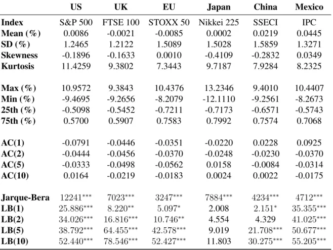
1.4.1 Stock Return Series Summary Statistics
We include 12 stock market indices in our estimations. These country / regional level
mar-ket indices are S&P 500 (US), FTSE 100 (UK), STOXX 50 (EU), Nikkei 225 (Japan), Shanghai
Stock Exchange Composite Index (China), IPC (Mexico), ASX All Ordinaries (Australia), Indice
Bovespa (Brazil), S&P / TSX Composite Index (Canada), DAX (Germany), CAC 40 (France), and
Hang Seng Index (Hong Kong). Developed markets and emerging markets are well-represented by
this list of chosen indices. The date range of the return series is from January 3rd, 2000 to October
30th, 2015. The stipulations of country specific holidays result in some fluctuations of the number
of trading days, which are generally close to 4000 days within the time window. A summary of the
return series is shown in Table 1.1 and Table 1.2. All reported values are raw daily returns rather
than annualized figures.
The tables indicate that three indices, namely the UK index FTSE 100, the EU index STOXX
50, and the French index CAC 40, have negative average daily return values. We notice that the all
of these are European indices. The tables also substantiate the existence of extreme returns. All
markets have experienced hikes and drastic declines within the scope of a day. Eight out of twelve
markets have seen a maximum daily return of over 10%, and maximum daily losses vary from
8.21% to 13.58%.1 Some of the most volatile trading days appeared in the Brazil, Hong Kong, and
Japan market. There have been instances in these markets where daily return was over 13% and
1Chinese stock market regulations restrict maximum daily price changes to 10% from the previous close for all A share
US UK EU Japan China Mexico
Index S&P 500 FTSE 100 STOXX 50 Nikkei 225 SSECI IPC
Mean (%) 0.0086 -0.0021 -0.0085 0.0002 0.0219 0.0445
SD (%) 1.2465 1.2122 1.5089 1.5028 1.5859 1.3271
Skewness -0.1896 -0.1633 0.0010 -0.4109 -0.2832 0.0349
Kurtosis 11.4259 9.3802 7.3443 9.7187 7.9284 8.2325
Max (%) 10.9572 9.3843 10.4376 13.2346 9.4010 10.4407
Min (%) -9.4695 -9.2656 -8.2079 -12.1110 -9.2561 -8.2673
25th (%) -0.5098 -0.5452 -0.7211 -0.7173 -0.6571 -0.5743
75th (%) 0.5700 0.5907 0.7583 0.7992 0.7574 0.7068
AC(1) -0.0791 -0.0446 -0.0351 -0.0220 0.0228 0.0925
AC(2) -0.0444 -0.0456 -0.0370 -0.0248 -0.0230 -0.0370
AC(5) -0.0333 -0.0498 -0.0562 0.0158 -0.0084 -0.0314
AC(10) 0.0164 -0.0219 -0.0183 0.0024 0.0022 -0.0175
Jarque-Bera 12241∗∗∗ 7023∗∗∗ 3247∗∗∗ 7884∗∗∗ 4234∗∗∗ 4712∗∗∗
LB(1) 25.886∗∗∗ 8.220∗∗ 5.097∗ 2.008 2.151∗ 35.355∗∗∗
LB(2) 34.026∗∗∗ 16.816∗∗∗ 10.746∗∗ 4.554 4.329 41.025∗∗∗
LB(5) 38.792∗∗∗ 64.455∗∗∗ 42.578∗∗∗ 9.019 21.708∗∗∗ 50.677∗∗∗
LB(10) 52.440∗∗∗ 78.546∗∗∗ 52.427∗∗∗ 11.803 30.275∗∗∗ 55.205∗∗∗
Table 1.1: Market Indices Summary Statistics: Jan. 3, 2000 - Oct. 30, 2015
daily loss was over 12%.
The Jarque-Bera normality test statistic is strongly significant for all indices, rejecting the null
hypothesis of normally distributed return series. The majority of these indices display negative
skewness, with the exceptions of the Mexican index IPC, the EU index STOXX 50, and the French
index CAC 40. Furthermore, it is evident that all return series are leptokurtic. The Canadian TSX
index and the Hong Kong Hang Seng Index have the highest sample kurtosis, followed by S&P
500. These observations are consistent with stylized facts that have been well documented in the
literature.
Lastly, we make the remark that all the autocorrelation coefficients of these series are quite
small and tend to be negative at one lag. The exceptions are China and Brazil, which are both
emerging markets. We show the Ljung-Box test statistics for 1, 2, 5, and 10 lags in the table. The
Australia Brazil Canada Germany France Hong Kong
Index ASX IBOV TSX DAX CAC 40 HSI
Mean (%) 0.0129 0.0241 0.0115 0.0115 -0.0046 0.0064
SD (%) 0.9689 1.7860 1.1333 1.5295 1.4876 1.5008
Skewness -0.5969 -0.0922 -0.6630 -0.0186 0.0050 -0.0791
Kurtosis 9.3706 7.1300 12.5073 7.4035 7.7770 11.4663
Max (%) 5.3601 13.6794 9.3703 10.7975 10.5946 13.4068
Min (%) -8.5536 -12.0961 -9.7880 -8.8747 -9.4715 -13.5820
25th (%) -0.4315 -0.9284 -0.4726 -0.7165 -0.7130 -0.6429
75th (%) 0.5168 1.0482 0.5738 0.7604 0.7489 0.7043
AC(1) -0.0154 -0.0019 -0.0131 -0.0201 -0.0337 -0.0134
AC(2) -0.0001 -0.0257 -0.0507 -0.0172 -0.0365 0.0050
AC(5) 0.0052 -0.0130 -0.0807 -0.0469 -0.0590 -0.0184
AC(10) 0.0061 0.0239 0.0295 -0.0147 -0.0234 -0.0379
Jarque-Bera 7229∗∗∗ 2941∗∗∗ 15857∗∗∗ 3337∗∗∗ 3927∗∗∗ 12339∗∗∗
LB(1) 0.984 0.014 0.706 1.666 4.694∗ 0.747
LB(2) 0.984 2.752 11.316∗∗ 2.890 10.207∗∗ 0.852
LB(5) 6.430 7.164 42.044∗∗∗ 20.011∗∗ 43.967∗∗∗ 4.016
LB(10) 10.122 15.973 56.120∗∗∗ 23.881∗∗ 55.936∗∗∗ 19.995∗
Table 1.2: Market Indices Summary Statistics: Jan. 3, 2000 - Oct. 30, 2015
Hong Kong indices. Nonetheless, we detect its presence in the other eight market return series.
1.4.2 Parameter Estimates and Test Statistics
In the sections to follow, we highlight some results for S&P 500 and leave the more
compre-hensive outputs in Appendix A.1. Parameter estimates from the symmetric absolute value and
asymmetric slope specifications are shown in Table 1.3. The quantile autoregressive term is
posi-tive for the 5% conditional quantile and negaposi-tive for the 1% conditional quantile, and the estimates
are significant in general. The coefficient terms associated with past returns are generally
signifi-cantly negative. Notably however, the responses to positive and negative returns from the previous
period are indeed different based on the asymmetric slope form.
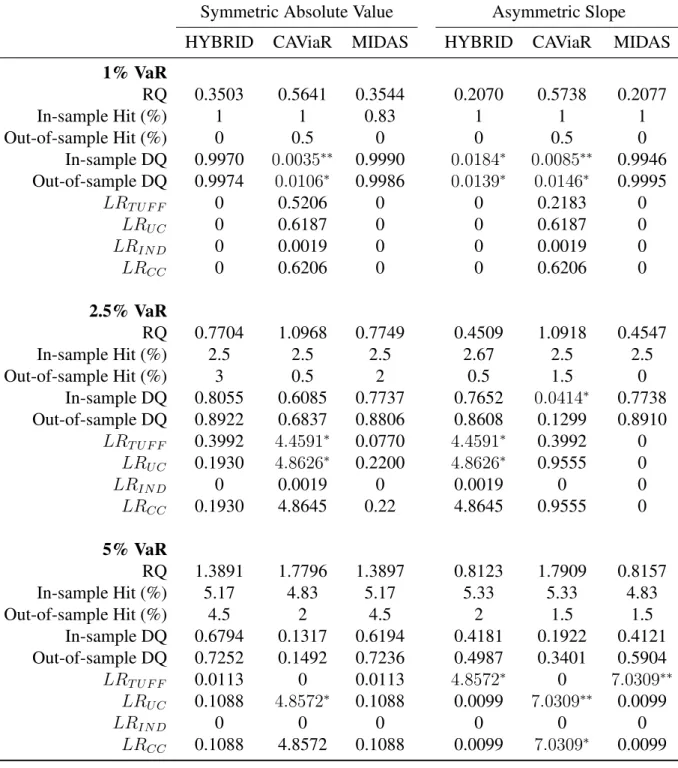
We report the corresponding coverage backtests in Table 1.4. When inspecting the DQ
statis-tics, we would like to see high p-values and to not be able to reject the null. This indicates that the
Symmetric Absolute Value Asymmetric Slope
HYBRID CAViaR MIDAS HYBRID CAViaR MIDAS
1% VaR
β1 -0.0211 -0.0368 -0.0098 -0.0229 -0.0220 -0.0216
β2 -0.1646 0.0586 -4.4038 -0.0365 2.7570 0.9786
(0.0212) (0.0298) (0.3407) (0.0036) (0.0004) (0.4172)
β3 -4.4500 -1.6091 2.8095 -4.9970 0.0247
(0.5983) (0.0869) (0.6338) (0.0047) (0.1154)
β4 -5.1768 1.4091
(0.2555) (0.0026)
κ1 2.8647 2.6071 1.2520 1.0145
(0.0283) (0.0131) (0.0096) (0.0100)
κ2 1.6350 1.6685
(0.0096) (0.0093)
5% VaR
β1 -0.0040 -0.0196 -0.0048 -0.0103 -0.0116 0.0344
β2 0.0231 0.2042 -3.6076 0.0751 2.9347 0.9243
(0.0242) (0.0234) (0.5237) (0.0042) (0.0007) (0.4358)
β3 -3.6216 -0.7652 3.0303 -5.4800 -0.0330
(0.4444) (0.0400) (0.5730) (0.0041) (0.3748)
β4 -5.4975 1.5219
(0.4369) (0.0016)
κ1 2.4455 2.4410 1.5647 0.0430
(0.0235) (0.0232) (0.0169) (0.0095)
κ2 1.6364 1.7339
(0.0109) (0.0056)
Symmetric Absolute Value Asymmetric Slope
HYBRID CAViaR MIDAS HYBRID CAViaR MIDAS
1% VaR
RQ 0.3503 0.5641 0.3544 0.2070 0.5738 0.2077
In-sample Hit (%) 1 1 0.83 1 1 1
Out-of-sample Hit (%) 0 0.5 0 0 0.5 0
In-sample DQ 0.9970 0.0035∗∗ 0.9990 0.0184∗ 0.0085∗∗ 0.9946 Out-of-sample DQ 0.9974 0.0106∗ 0.9986 0.0139∗ 0.0146∗ 0.9995
LRT U F F 0 0.5206 0 0 0.2183 0
LRU C 0 0.6187 0 0 0.6187 0
LRIN D 0 0.0019 0 0 0.0019 0
LRCC 0 0.6206 0 0 0.6206 0
2.5% VaR
RQ 0.7704 1.0968 0.7749 0.4509 1.0918 0.4547
In-sample Hit (%) 2.5 2.5 2.5 2.67 2.5 2.5
Out-of-sample Hit (%) 3 0.5 2 0.5 1.5 0
In-sample DQ 0.8055 0.6085 0.7737 0.7652 0.0414∗ 0.7738
Out-of-sample DQ 0.8922 0.6837 0.8806 0.8608 0.1299 0.8910
LRT U F F 0.3992 4.4591∗ 0.0770 4.4591∗ 0.3992 0
LRU C 0.1930 4.8626∗ 0.2200 4.8626∗ 0.9555 0
LRIN D 0 0.0019 0 0.0019 0 0
LRCC 0.1930 4.8645 0.22 4.8645 0.9555 0
5% VaR
RQ 1.3891 1.7796 1.3897 0.8123 1.7909 0.8157
In-sample Hit (%) 5.17 4.83 5.17 5.33 5.33 4.83
Out-of-sample Hit (%) 4.5 2 4.5 2 1.5 1.5
In-sample DQ 0.6794 0.1317 0.6194 0.4181 0.1922 0.4121
Out-of-sample DQ 0.7252 0.1492 0.7236 0.4987 0.3401 0.5904
LRT U F F 0.0113 0 0.0113 4.8572∗ 0 7.0309∗∗ LRU C 0.1088 4.8572∗ 0.1088 0.0099 7.0309∗∗ 0.0099
LRIN D 0 0 0 0 0 0
LRCC 0.1088 4.8572 0.1088 0.0099 7.0309∗ 0.0099
predicting the 1% VaR, the CAViaR model has significant DQ values under both specifications.
HYBRID also yields an inferior performance compared to MIDAS, which does not reject the null
hypothesis in any case. For the 2.5% VaR, the DQ test null hypothesis is only rejected once under
the asymmetric slope form of CAViaR. None of the out-of-sample DQ tests reject the null
hy-pothesis. Model performances further improve over 5% VaR predictions, and none rejects the null
hypothesis. We infer that MIDAS is the best model using the DQ test criterion. Additionally, it
appears that the adaptive form is the least accurate when judged by the DQ tests and we leave it
out of the main discussion (see Appendix A.1).
Furthermore, we evaluate model performances upon the likelihood ratio tests. The relevant
critical values areχ2
0.05(1) = 3.84for the unconditional coverage, the time until first failure, and
the independence test, and χ2
0.05(2) = 5.99 for the joint test. We notice a few likelihood ratios
surpassing the critical values and mark them accordingly in the table. All models pass the
uncon-ditional coverage test, the time until first failure test, the independence test, as well as the joint
test at the 1% VaR level. At the 2.5% level, MIDAS is the only model that passes all four tests
under all circumstances. HYBRID and CAViaR pass the joint tests, but fail the unconditional
coverage test respectively with the asymmetric slope and symmetric absolute value form. At the
5% level, CAViaR has the least adequate performance in the unconditional coverage test and fails
under both specifications. It also does not pass the joint test when the conditional quantile model
takes the asymmetric slope form. HYBRID and MIDAS manage to pass the three coverages tests
and the joint test, when the past returns are included in conditional quantile estimations as their
symmetric absolute values. Both pass the unconditional, independence, and joint coverage test
un-der the asymmetric slope model. The test outcomes for HYBRID and MIDAS are quite consistent
regardless of the functional form specification.
To better justify the addition of the MIDAS weighting polynomial, we perform another exercise
and present the results in Table 1.5. Under the specification denoted HYBRID-UM, we estimated
a coefficient for each of the 5 past returns separately instead of imposing the MIDAS weight. This
is essentially the U-MIDAS model derived by Foroni, Marcellino, and Schumacher (2013). DQ
less correctly identified than the ones from the HYBRID-quantile form. Through these two sets of
statistics, we establish that HYBRID and MIDAS are superior when estimating the lower tails, i.e.
1%, 2.5%, and 5% conditional quantiles, of the return series.
HYBRID HYBRID-UM MIDAS
5% VaR
In-sample DQ 0.6794 0.0084∗∗ 0.6194
Out-of-sample DQ 0.7252 0.0061∗∗ 0.7236
LRU C 0.1088 4.8572∗ 0.1088
LRIN D 0 0 0
LRCC 0.1088 4.8572∗ 0.1088
Table 1.5: Backtests - MIDAS vs. U-MIDAS Weights
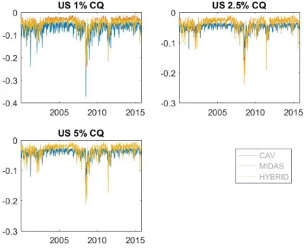
Figure 1.2 illustrates the 5% conditional quantiles of S&P 500, during the entire sample
win-dow of January 2000 to October 2015. We make the observation that the range of the quantiles
tends to remain stable in most time periods. However, there are also notable dips corresponding to
various occurrences of financial crisis. For example, this distinct pattern appears around the time
point of the 2008 - 2009 financial crisis. Furthermore, its impact can be seen across all markets
(see Appendix A.2). The plots therefore carry relevant information to depict downside risks in
various equity markets.
1.4.3 Benchmark Quantiles from GARCH-based Parametric Bootstrapping
In this section, we produce the conditional quantile values attained from the bootstrapping
process. We use these as the benchmark, and move forward to calculate and plot the implied
conditional asymmetry.
As stated in the model evaluation section, we adopt five GARCH-type models and three
distri-butions for the innovation term. The unconditional quantiles extrapolated from these specifications
are reported in Table 1.6 for the S&P 500 returns. All non-linear GARCH models produce lower
unconditional quantile values at the 1%, 2.5%, and 5% level, compared to the standard GARCH
model. Among different GARCH-type settings, GJR-GARCH and TGARCH generate the
GJR-GARCH / normal model, -6.36% under the TGARCH / skewed normal model, and -6.08%
under the TGARCH / student-t model. Overall, we also notice that using skewed normal
inno-vation terms lead to lower estimates of the unconditional quantiles. This suggests that adopting
alternative innovation terms is necessary for incorporating heavier tails.
Model Normal Skewed normal Student-t
1% Quantile (%)
GARCH -5.3900 -5.5455 -5.5090
EGARCH -5.8997 -6.1334 -5.9406
GJR-GARCH -6.0742 -6.3445 -5.9683
IGARCH -5.6265 -5.7603 -5.6443
TGARCH -6.0501 -6.3564 -6.0848
2.5% Quantile (%)
GARCH -4.6139 -4.6946 -4.6743
EGARCH -5.0231 -5.1606 -4.9750
GJR-GARCH -5.1652 -5.2517 -5.0553
IGARCH -4.7750 -4.8966 -4.7633
TGARCH -5.1239 -5.3361 -5.1011
5% Quantile (%)
GARCH -3.8670 -3.9147 -3.8390
EGARCH -4.1473 -4.2641 -4.1060
GJR-GARCH -4.2570 -4.2993 -4.1599
IGARCH -3.9763 -4.0592 -3.9130
TGARCH -4.2206 -4.3880 -4.1776
Table 1.6: Unconditional Quantiles from GARCH Parametric Bootstrapping - S&P 500
In Table A.13 to Table A.15 (see Appendix A.3), we summarize the 1%, 2.5%, and 5%
boot-strapped unconditional quantiles for all other markets. The return figures are adjusted by the
cor-responding exchange rates between the currency denominations of the indices and the U.S. dollar.
These return quantiles are more or less consistent with the summary statistics of the return series.
One notable case is Brazil, whose 1%, 2.5%, and 5% quantiles are distinctly lower than the rest of
the series.
We compile loss value tables by market and by loss functions to gauge their performances. We
present the mean squared errors (MSE) derived from the S&P 500 returns in Table 1.7, and leave
the symmetric absolute value specification, which stays consistent across the 1%, 2.5%, and 5%
conditional quantiles.
When allowing for different responses of conditional quantiles to past returns, i.e. the
asymmet-ric slope specification, CAViaR and MIDAS sometimes outperform HYBRID. More specifically,
CAViaR estimates are closer to the benchmarks when it comes to the 1% conditional quantiles
and MIDAS performs rather well in respect to estimating 5% conditional quantiles. HYBRID
ap-pears to be the optimal model under most scenarios nonetheless. Additionally, the decreases in
MSE when switching from CAViaR or MIDAS to HYBRID are pronounced. We reach the
simi-lar conclusion after examining mean absolute errors (MAE). We next inspect the results from the
exponential Bregman loss function, where we selecta = 1 and show an excerpt of the complete outputs in Table 1.8. We can see that HYBRID maintains its performances when we penalize
over-estimation of the lower return quantiles. The magnitudes of the loss values are similar to those of
mean squared error.
Overall, HYBRID yields satisfactory outcomes when the returns assume GARCH-type DGPs.
This finding is robust to various settings of the innovation term. We observe stronger performances
on 2.5% and 5% conditional quantile estimations. This is quite natural, as accurately estimating
the 1% conditional quantiles is perceived to be more difficult.
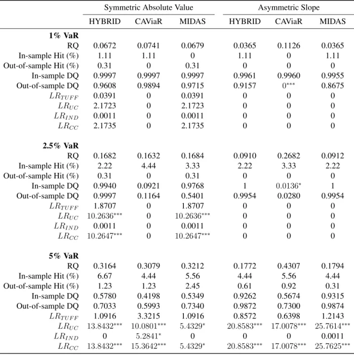
1.4.4 The Financial Crisis of 2008: An Event Study
Considering the impact of the 2008 financial crisis, we would like to direct our attention to a
sub-period within the 15-year span. We repeat the estimations carried out in previous sections with
data from September 2007 to October 2015. The in-sample period is set around the crisis, from
September 2007 to July 2009.
The parameter estimates do not seem to deviate much from those of the full sample. We
do observe, however, smaller impacts of negative returns on future conditional quantiles. The
unconditional coverage probabilities, on the other hand, indicate that the estimates are less robust
when put to the backtests. Clustering of extreme returns could have contributed to this outcome,
Symmetric Absolute Value Asymmetric Slope
HYBRID CAViaR MIDAS HYBRID CAViaR MIDAS
GARCH
Normal 1% 0.0005 0.0015 0.0007 0.0010 0.0007 0.0010
2.5% 0.0002 0.0013 0.0005 0.0004 0.0004 0.0005
5% 0.0002 0.0010 0.0002 0.0003 0.0003 0.0002
Skewed-normal 1% 0.0005 0.0017 0.0007 0.0010 0.0008 0.0010
2.5% 0.0002 0.0014 0.0006 0.0004 0.0004 0.0005
5% 0.0002 0.0011 0.0002 0.0003 0.0003 0.0002
Student-t 1% 0.0005 0.0016 0.0008 0.0011 0.0008 0.0011
2.5% 0.0002 0.0014 0.0006 0.0005 0.0005 0.0006
5% 0.0002 0.0010 0.0002 0.0003 0.0004 0.0002
EGARCH
Normal 1% 0.0007 0.0016 0.0009 0.0011 0.0007 0.0011
2.5% 0.0004 0.0013 0.0007 0.0005 0.0004 0.0006
5% 0.0003 0.0009 0.0003 0.0003 0.0003 0.0002
Skewed-normal 1% 0.0008 0.0019 0.0010 0.0011 0.0008 0.0011
2.5% 0.0004 0.0015 0.0008 0.0005 0.0005 0.0006
5% 0.0003 0.0010 0.0003 0.0004 0.0003 0.0002
Student-t 1% 0.0007 0.0017 0.0009 0.0010 0.0007 0.0011
2.5% 0.0004 0.0014 0.0008 0.0005 0.0005 0.0007
5% 0.0003 0.0009 0.0003 0.0004 0.0003 0.0003
GJR-GARCH
Normal 1% 0.0007 0.0019 0.0011 0.0011 0.0009 0.0012
2.5% 0.0004 0.0015 0.0008 0.0006 0.0006 0.0007
5% 0.0003 0.0010 0.0004 0.0004 0.0004 0.0003
Skewed-normal 1% 0.0008 0.0021 0.0012 0.0010 0.0009 0.0012
2.5% 0.0004 0.0016 0.0008 0.0006 0.0006 0.0007
5% 0.0003 0.0010 0.0003 0.0004 0.0004 0.0003
Student-t 1% 0.0007 0.0020 0.0010 0.0011 0.0009 0.0012
2.5% 0.0004 0.0015 0.0007 0.0006 0.0006 0.0001
5% 0.0003 0.0010 0.0004 0.0004 0.0004 0.0003
Symmetric Absolute Value Asymmetric Slope
HYBRID CAViaR MIDAS HYBRID CAViaR MIDAS
GARCH
Normal 1% 0.0004 0.0014 0.0006 0.0009 0.0007 0.0009
2.5% 0.0002 0.0012 0.0005 0.0004 0.0004 0.0004
5% 0.0002 0.0010 0.0002 0.0003 0.0003 0.0002
Skewed-normal 1% 0.0005 0.0016 0.0007 0.0009 0.0007 0.0009
2.5% 0.0002 0.0013 0.0005 0.0004 0.0004 0.0004
5% 0.0002 0.0010 0.0002 0.0003 0.0003 0.0002
Student-t 1% 0.0005 0.0015 0.0007 0.0010 0.0008 0.0010
2.5% 0.0002 0.0013 0.0005 0.0005 0.0005 0.0005
5% 0.0002 0.0010 0.0002 0.0003 0.0003 0.0002
EGARCH
Normal 1% 0.0007 0.0016 0.0008 0.0010 0.0007 0.0010
2.5% 0.0004 0.0013 0.0007 0.0005 0.0004 0.0006
5% 0.0003 0.0009 0.0003 0.0003 0.0003 0.0002
Skewed-normal 1% 0.0007 0.0018 0.0009 0.0010 0.0007 0.0010
2.5% 0.0004 0.0014 0.0008 0.0005 0.0005 0.0006
5% 0.0003 0.0010 0.0003 0.0003 0.0003 0.0002
Student-t 1% 0.0006 0.0017 0.0009 0.0009 0.0007 0.0010
2.5% 0.0004 0.0013 0.0007 0.0005 0.0005 0.0006
5% 0.0003 0.0009 0.0003 0.0004 0.0003 0.0002
GJR-GARCH
Normal 1% 0.0006 0.0018 0.0010 0.0010 0.0008 0.0011
2.5% 0.0004 0.0015 0.0007 0.0006 0.0006 0.0007
5% 0.0003 0.0010 0.0003 0.0004 0.0004 0.0003
Skewed-normal 1% 0.0008 0.0020 0.0011 0.0009 0.0008 0.0011
2.5% 0.0004 0.0015 0.0007 0.0005 0.0005 0.0006
5% 0.0003 0.0010 0.0003 0.0003 0.0004 0.0002
Student-t 1% 0.0006 0.0018 0.0010 0.0010 0.0008 0.0011
2.5% 0.0004 0.0015 0.0007 0.0006 0.0006 0.0007
5% 0.0003 0.0010 0.0003 0.0004 0.0004 0.0003
Symmetric Absolute Value Asymmetric Slope
HYBRID CAViaR MIDAS HYBRID CAViaR MIDAS
1% VaR
β1 -0.0496 -0.0059 -0.0478 -0.0288 -0.1293 -0.0289
(0.0003) (0.0000) (0.0000) (0.0000) (0.0001) (0.0000)
β2 -0.0512 1.0479 -1.9319 0.0113 0.1399 2.1096
(0.0441) (0.0001) (0.0615) (0.0269) (0.0065) (0.8832)
β3 -2.0203 0.3039 2.0893 0.0875 -3.7116
(0.2326) (0.0014) (0.8452) (0.0314) (0.0858)
β4 -3.6555 0.0460
(0.1230) (0.2941)
2.5% VaR
β1 -0.0473 -0.0049 -0.0463 -0.0288 -0.0403 -0.0287
(0.0006) (0.0000) (0.0001) (0.0001) (0.0002) (0.0000)
β2 -0.0137 1.1386 -1.9509 0.0275 0.3383 2.1297
(0.0917) (0.0014) (0.1605) (0.0487) (0.0479) (1.4374)
β3 -1.9608 0.4509 2.0223 0.0103 -3.7551
(0.6308) (0.0059) (1.6019) (0.0388) (0.1410)
β4 -3.5075 0.0400
(0.3707) (0.0858)
5% VaR
β1 -0.0139 -0.0031 -0.0082 -0.0172 0.0498 -0.0208
(0.0002) (0.0000) (0.0001) (0.0001) (0.0000) (0.0001)
β2 -0.1542 1.1531 -3.6338 0.0831 0.9220 2.3545
(0.0540) (0.0029) (0.9695) (0.0307) (0.0029) (1.9794)
β3 -3.8988 0.3736 3.2142 -0.0483 -4.4611
(1.1667) (0.0061) (1.4435) (0.0160) (0.2003)
β4 -4.9923 0.0617
(1.8121) (0.0074)
Symmetric Absolute Value Asymmetric Slope
HYBRID CAViaR MIDAS HYBRID CAViaR MIDAS
1% VaR
RQ 0.0672 0.0741 0.0679 0.0365 0.1126 0.0365
In-sample Hit (%) 1.11 1.11 0 1.11 0 1.11
Out-of-sample Hit (%) 0.31 0 0.31 0 0 0
In-sample DQ 0.9997 0.9997 0.9997 0.9961 0.9960 0.9955
Out-of-sample DQ 0.9608 0.9894 0.9715 0.9157 0∗∗∗ 0.8675
LRT U F F 0.0391 0 0.0391 0 0 0
LRU C 2.1723 0 2.1723 0 0 0
LRIN D 0.0011 0 0.0011 0 0 0
LRCC 2.1735 0 2.1735 0 0 0
2.5% VaR
RQ 0.1682 0.1632 0.1684 0.0910 0.2682 0.0912
In-sample Hit (%) 2.22 4.44 3.33 2.22 3.33 2.22
Out-of-sample Hit (%) 0.31 0 0.31 0 0 0
In-sample DQ 0.9940 0.0921 0.9768 1 0.0136∗ 1
Out-of-sample DQ 0.9997 0.1164 0.5401 0.9954 0.0280 0.9954
LRT U F F 1.8707 0 1.8707 0 0 0
LRU C 10.2636∗∗∗ 0 10.2636∗∗∗ 0 0 0
LRIN D 0.0011 0 0.0011 0 0 0
LRCC 10.2647∗∗∗ 0 10.2647∗∗∗ 0 0 0
5% VaR
RQ 0.3164 0.3079 0.3212 0.1772 0.4307 0.1794
In-sample Hit (%) 6.67 4.44 5.56 4.44 5.56 4.44
Out-of-sample Hit (%) 1.23 1.23 2.45 0.61 0.92 0.31
In-sample DQ 0.5780 0.4198 0.5349 0.9262 0.5674 0.9315
Out-of-sample DQ 0.7033 0.5993 0.7340 0.9872 0.7300 0.9874
LRT U F F 1.0916 3.3215 1.0916 0.8572 0.6398 1.2143 LRU C 13.8432∗∗∗ 10.0801∗∗∗ 5.4329∗ 20.8583∗∗∗ 17.0078∗∗∗ 25.7614∗∗∗
LRIN D 0 5.2841∗ 0 0 0 0.0011
LRCC 13.8432∗∗∗ 15.3642∗∗∗ 5.4329∗ 20.8583∗∗∗ 17.0078∗∗∗ 25.7625∗∗∗
1.4.5 Conditional Asymmetry
Having obtained conditional quantile estimates, we would like to explore the conditional
asym-metry in the underlying distributions of the multi-period returns. Conditional asymasym-metry indicates
the direction of conditional skewness in underlying asset returns. The concept can be traced back
to Bowley (1920)
CAθ(rt,n) =
[q1−θ(rt,n)−q0.50(rt,n)]−[q0.50(rt,n)−qθ(rt,n)] q1−θ(rt,n)−qθ(rt,n)
, (1.4.1)
whereqθ(rt,n), q1−θ(rt,n)andq0.50(rt,n)represent theθ-th, (1 - θ)-th unconditional quantiles and
the unconditional median of the return. We define a similar measure using conditional quantiles
(White, Kim & Manganelli, 2008)
CAθ,t(rt,n) =
[q1−θ,t(rt,n)−q0.50,t(rt,n)]−[q0.50,t(rt,n)−qθ,t(rt,n)] q1−θ,t(rt,n)−qθ,t(rt,n)
. (1.4.2)
This is the conditional counterpart ofCAθ(rt,n).
Fig. 1.3: Conditional Asymmetry - US
market indices (see Appendix A.5). The plot for S&P 500 are shown in Figure 1.3 as an example.
The graphs suggest that on a weekly basis, there tends to be a considerable amount of fluctuation
in this measure. At the end of the time window that we examine, conditional asymmetry values
produced by all models have evolved to be negative. Market indices are shown to be left-skewed
conditionally.
1.5 Portfolio Construction
A trading strategy built upon the conditional asymmetry of equity returns is devised in this
section. Our intention is to inspect the risk and return implied by such strategy, and justify the
diversification approach.
We start by identifying the conditional value-at-risk (CVaR) optimal portfolio. We adopt
con-ditional VaR as the portfolio risk proxy that we intend to minimize in the optimization process.
This approach follows Rockafellar and Uryasev (2000). The portfolio optimization problem is set
up with a collection of N assetsx1, ..., xN and returnsr1, ..., rN. For a specified probability level α, we would like to find the portfolio x that minimizes
CV aRβ(x, α) =α+
1 1−β
Z
r∈RN
[f(x, r)−α]+p(r)dr. (1.5.1)
Heref(x, r) = −xTris the loss function, p(r)is the probability density function of asset return, β is a given probability level, andαis the value-at-risk associated with β. Equivalently, we have
α= min{α:P r[f(x, r)≤β]≥α}.
We place the constraint that there is no short-selling allowed for the Chinese market index,
and allow at most three times leverage. In other words, the portfolio weights{wi}i=1,2,3,4,5should
satisfy
5
X
i=1
wi = 1, w1, w2, w3, w4 ≥ −1, w5 ≥0. (1.5.2)
For cases other than the baseline portfolio, we adjust asset returns by
ri,CA =ri ×(1 +
CAi
P
i|CAi|
Through this adjustment, we are favoring assets with a positive conditional asymmetry or a
neg-ative conditional asymmetry with a smaller magnitude. To make sure that the time windows are
consistent for all assets, we calculate the 4-week moving average of the weekly returns and keep
700 such values for all indices. We perform portfolio optimization and analysis by month, year,
and with all observations. These smaller time windows are non-overlapping. To demonstrate the
composition of representative portfolios generated by different models, we list the average weights
assigned to each asset in Table 1.11 by rebalancing frequency.
Frequency US UK EU Japan China
Monthly
Base CVaR 0.2602 0.3013 0 0.0986 0.3399
HYBRID CA5 0.3596 0.1297 0 0.2584 0.2523
CAV CA5 0.2899 0.0646 0.2268 0.0841 0.3346
MIDAS CA5 0.1938 0.1652 0.0403 0.3011 0.2997
Annual
Base CVaR 0.2733 0.2939 0 0.0958 0.3371
HYBRID CA5 0.4124 0.1036 0.2653 0.1141 0.1046
CAV CA5 0.3126 0.0626 0.2391 0.0836 0.3022
MIDAS CA5 0.2216 0.1579 0.0327 0.3102 0.2777
Overall
Base CVaR 0.3565 0.2538 0 0.0964 0.2933
HYBRID CA5 0.4129 0.1527 0.2242 0.1251 0.0851
CAV CA5 0.4500 0 0.2820 0 0.2680
MIDAS CA5 0.2873 0.1639 0.0346 0.2650 0.2491
Table 1.11: Asset Allocation Summary
From a monthly perspective, asset weights tend to fluctuate over the 175 portfolios. Hence the
monthly representative portfolio is slightly different from that of annual and overall
representa-tive portfolios. When adjusted by the 5% quantile conditional asymmetry, the monthly HYBRID
representative portfolio shifts asset weights away from the UK and the Chinese indices to the US
and the Japan markets. The resulting portfolio is significantly more heavily invested in the latter
two market indices, with weights changing from 26.02% to 35.96% and from 9.86% to 25.84%
underweighting the UK index in the CAViaR and the MIDAS design. The CAViaR portfolio holds
the largest long position in the European market, whereas the MIDAS portfolio tilts towards the
Japanese market.
When placed under an annual rebalancing scheme, the HYBRID representative portfolio shifts
asset weights away from the UK, Japanese, and Chinese indices to the US and EU indices after
accounting for the 5% return quantile conditional asymmetry. The portfolio allocation favors the
US market index, with a weight change from 35.96% to 41.24%. The CAViaR portfolio and the
MIDAS portfolio are both more concentrated in the Chinese market, with an allocation of 30.22%
and 27.77% respectively. In addition, the CAViaR holdings are mainly distributed to the U.S. and
the EU market and the MIDAS holdings are mostly in the U.S. and Japan.
Using all the data in the 700-week range to calculate asset weights, an increase in the US index
position holds true for all portfolio designs. This is also the case for the EU market index in the
CAViaR and the MIDAS portfolio. The HYBRID portfolio takes slightly large stakes in the UK
and Japanese indices, and indicates a downward weight adjustment in the Chinese index for 1.95%.
We compare the risk and return characteristics of the HYBRID, CAViaR, and MIDAS
portfo-lios, along with the baseline CVaR portfolio and the equal-weight portfolio. Annualized return,
risk, and their Sharpe ratios are displayed in Table 1.12. We assume a zero risk-free rate in Sharpe
ratio calculation, which is quite realistic in the current economic environment. Judging from the
risk-return tradeoff, both the HYBRID and the MIDAS portfolio outperform the default CVaR
optimal portfolio, the equal-weight portfolio, as well as the CAViaR portfolio. The improvement
from the HYBRID portfolio based on the5%conditional quantile adjustment is the most distinct.
rp σp Sharpe Ratio
Base CVaR 4.68 7.13 0.66
Equal-weight 5.25 7.65 0.69
HYBRID CA5 7.85 7.38 1.06
CAV CA5 4.55 7.72 0.59
MIDAS CA5 6.91 7.49 0.92
1.6 Concluding Remarks
Evaluated by three different backtesting measures, we have established that the HYBRID-SAV
model has the strongest performance when predicting the 5% conditional quantiles for various
GARCH-type models. Additionally, we directed our attention to the 2008 financial crisis as an
event study. Along the lines of minimizing conditional value-at-risk, we have also identified a
portfolio allocation based on returns adjusted by the 5% conditional asymmetry measures. As part
of the future work, we would like to further improve the accuray and forecasting power of the
HYBRID model. This would enable us to expand the use of the model to general prediction of
conditional quantiles and beyond tail events. We would also like to develop other trading strategies
2 Has the Downside Risk in the Chinese Stock Market Fundamentally Changed?
2.1 Introduction
Stock market trading in mainland China takes place on two stock exchanges, namely the
Shang-hai Stock Exchange and the Shenzhen Stock Exchange. Both have been in existence for roughly 25
years, with an inception date of December 19, 1990 for Shanghai and July 3, 1991 for Shenzhen.
Along with the rapid development of the Chinese economy, the two stock exchanges have grown
to be respectively the 4th and the 7th largest in the world based on market capitalization.
A number of features set the Chinese market apart from western stock exchanges. First,
al-though on par in terms of trading volume and market size, the mainland Chinese stock market is
predominantly driven by retail trading. Second, there is the lingering issue of market transparency
and regulatory uncertainty. Various changes were implemented through time discussed later
-aimed at reducing the opaqueness of the market. Third, recent tumultuous behavior of the broad
equity indices, with a 40 percent drop of the Shanghai Composite index during the summer of
2015, prompted a government sponsored buying spree.1
While there already exists a number of studies about the Shanghai and Shenzhen Stock
Ex-changes, to the best of our knowledge we are not aware of an in-depth study of downside risks
in Chinese equity markets. Downside risk is a serious concern for traders, but more broadly the
notion that a major market correction can or will happen has kept both the financial professionals
and political leaders on alert. The purpose of the paper is to characterize fundamental changes
-if any - in the downside risk of the Chinese stock market and discern what are the causes of these
changes.
1In particular, China’s so called “national team” owned at least 6 per cent of the mainland stock market as a result