IEE Irish Signals and Systems Conference, Dublin, June 28-30, 2006
Analysis of Trend in Vehicular Traffic Flow Data by
Wavelets
Bidisha Ghosh, Biswajit Basu
*and
Margaret O’Mahony
Department of Civil, Structural and Environmental Engineering Trinity College, Dublin
IRELAND
E-Mail Address: [email protected]*
___________________________________________________________________________________ _______
This paper proposes a method to model the daily trend in vehicular traffic flow data using a wavelet transform technique. The approach in this paper first decomposes the historical traffic volume to an approximate part associated with low frequency fluctuations and several detailed parts associated with high frequency fluctuations by means of discrete wavelet transform. The approximate part, averaged over a few days, represents the daily trend of traffic flow. The high frequency parts are separately modelled and added to the trend to get an approximate nature of the traffic flow over a day. A case study is performed at a traffic junction in Dublin with the proposed approach.
___________________________________________________________________________________ _______
I INTRODUCTION
In any transportation network, the implementation of Intelligent Transportation Systems (ITS) involves collection of a huge amount of traffic condition related data for real-time monitoring and operational purpose. The two important aspects of ITS, Advanced Traffic Management Systems (ATMS) and Advanced Traveller Information Systems (ATIS) require continuous forecasting of traffic conditions in near (short-term) future based on the current scenario. The major existing Urban Traffic Control Systems (UTCS) (like, SCATS and SCOOTS) use the simple random walk model for the purpose of forecasting as a part of ITS. A significant amount of research has been conducted to improve the real-time applicability of short-term forecasting techniques in relation to ITS. Extensive review on this subject is available from the studies of Van Arem [1] and Vlahogianni [2]. The well known short-term forecasting techniques include non-parametric regressions (e.g. [3]), neural networks (e.g. [4]), linear and non-linear regression, historical average algorithms (e.g. [5]), ARIMA time-series models (e.g. [6]). All the well-known short-term forecasting techniques are generally dependent on large datasets including
information on current traffic data to forecast the near future.
This paper develops a unique technique to develop a traffic flow modelling methodology based on the trend underlying the traffic flow over a day. The random variations over the trend are modelled by much simpler time-series techniques. Instead of point prediction or interval prediction, the basic trend along with the random variation represents the daily traffic flow. This model may not have better or equal accuracy as compared to other complicated statistical methodologies often used in short-term traffic prediction, but will be useful to obtain a simple yet reasonably accurate model which can represent the existing traffic condition.
applicable to the vehicular traffic as variations of traffic flow at different time scales are generated due to different factors. Further, the advantage of the application of wavelet analysis is in the inherent capability of accounting for non-stationary time-series which is usually dealt with separately in conventional time-series model.
This paper is organized as follows: Section 2 presents the proposed methodology. Section 3 describes the case study in Dublin and the results are shown in section 4. Finally, Section 5 concludes the paper.
II METHODOLOGY
a)
Wavelet Transform
Wavelet analysis decomposes a signal X(t) to a linear combination of shifted and scaled versions of the original (or mother) wavelet. Discrete wavelet transform (DWT) consists of the collection of coefficients:
, , , J Jk j jkc k X t
j k Z
d k X t
(1)
where <∗,∗> denotes the inner product,
dj k
are the detail coefficients at level j (j = 1,2,…J) and
cJ
k
are the approximate coefficients at level J. The signal X to be analyzed is integrally transformed with a set of basis functions
2 2
2
j j
jk t t k
(2)
which is constructed from the mother-wavelet (t) by a time-shift operation and a dilation operation. The function jk
t is a time shifted version of the mother scaling function
:
j t jk t j t k
. The wavelet,
j t
is a low-pass function which can separate the low frequency component of the signal. Thus, DWT decomposes a signal into a large timescale (low frequency) approximation and a collection of details at different smaller timescales (higher frequencies).
Discrete Wavelet Transform (DWT) ‘daubechies’ 4' is used here to decompose the signal into different time scales. Initially, the original traffic volume data over a few days are decomposed into approximation coefficients c1
and detail coefficients d1. The approximation
coefficients c1 are again decomposed to
approximation coefficients c2 and detail
coefficients d2 at the next level. This procedure
is repeated for further decomposition.
The original signal can be reconstructed back from the decomposed approximation and the detail components. Thus, the original signal can be represented as,
J
j
j J
X t A t D t
(3)where, A tJ
is the reconstruction of the approximation coefficients cJ at level J and
j
D t is the reconstruction obtained from the detail coefficients dj at level j. In the
reconstructed approximation (AJ) and in the
reconstructed details obtained at each stage/level (D1,D2, D3… DJ) the numbers of
data points remain the same as the original data set.
The aim of repeating the decomposition procedure is to find an optimum approximation level. The optimum approximation level signifies a smoothed representation of the traffic data which can truly represent the trend in a general day’s traffic flow pattern. Daily traffic is affected by several uncontrollable factors for example, weather etc. So, to obtain the ‘trend over a day’, the average of the approximation values over a few days is taken instead of a single day.
The trend obtained in this way is unique in the sense that it has not been obtained by curve-fitting, polynomial fitting or regression techniques. The trend is reported in a non-analytical functional form and has better flexibility in representation.
Though obtaining a representative ‘trend’ over a day of traffic flow is the main feature of the analysis, for better accuracy the high frequency ‘details’ parts are also modelled. Generally these high frequency components are random in nature. But with an increase in decomposition level, self-similar nature can be observed in them.
III CASE STUDY AND ANALYSIS
a)
The Traffic Flow Data
essentially carried out on the data observed during weekdays. Since, the data set used does not contain any missing data, no special treatment for missing data is required to be utilised here. A plot of the traffic flow data in vehicles per hour (vph) against time is ahown in figure 1.
Figure 1:Traffic flow observations over a week at junction TCS183
The traffic flow data plot shows a stationary nature. Wavelet can handle non-stationarity and unlike other time-series modeling techniques where this issue is required to be separately dealt with and transformation of data is required to be performed [9].
b)
Wavelet Decomposition
Figure 2:Approximation at level 3 and details at level 1, 2, 3 over 3 consecutive days
The traffic flow data over ten days i.e. two weeks (as weekends are not included), are decomposed into three levels at three different time scales, approximately 45 min, 11
2 hours and 3 hours using Discrete Wavelet Transform (DWT) with Daubechie-4 wavelet basis as described in section II. The approximation obtained at the third level is considered as the optimum level of approximation. The wavelet coefficients for approximation and detail are then reconstructed and for modeling purpose the reconstructed values are always used in this paper. The high frequency part of the data are separated at these three levels. The low frequency part at level three is quite smooth and can be used as a representative of the overall trend over a day in the traffic data. The approximations at level three, i.e. over three hours and the details at 45 min, 11
2 hours and 3 hours over a day are plotted in figure 2.
c)
Trend Modelling
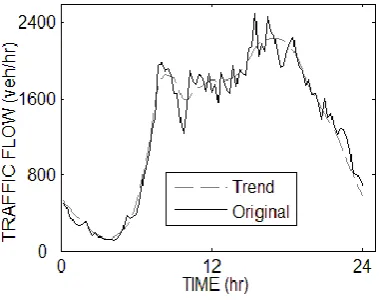
[image:3.595.315.505.465.615.2]To model a representative trend, Level 3 approximations over 10 days are taken. An average of 10 days is used to eliminate the influence of any unusual incident occurrence or other uncontrolled effects such as, weather effects. The average over ten days is then considered as a true daily trend for the particular approach at TCS183.
Figure 3:Trend and original observations on an arbitrary day
[image:3.595.91.281.470.731.2]the details in three levels can give approximately 80% accurate result (2σ = 76, σ being the standard deviation; which is approximately 20% of 330). For better accuracy the detailed parts are modelled in the following section.
[image:4.595.89.281.171.400.2]d)
Modelling of Details
Figure 4:Correlogram of details at level 1, 2 and 3 over 10 consecutive days
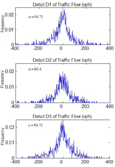
Figure 5:Histogram of details at level 1, 2 and 3 over 10 consecutive days
The ‘daily trend’ obtained above can be a good approximation of the daily traffic. But totally ignoring the high frequency part of the daily traffic may not give a satisfactory model.
The high frequency data obtained at three different levels are first checked to find any existing autocorrelation in each series. The correlogram at each detailed level are plotted in figure 4. From the plots, D1 seems to be
white noise and D2, D3 can be modelled using
time-series as done in [8].
As the main aim of the paper is to develop a simple modelling technique, the simplest possible time-series models are employed to predict the future. The details at different levels are modelled separately as Gaussian noise.
Figure 5 shows the histogram plot of the details at three levels. The variances of all three of the details are quite comparable. To develop a reasonably accurate, simple and parsimonious model for the random variation only one level of details are decided to be considered. As the standard deviation for the residual was 38 (Section IIIc), ignoring the other two levels of the details may only cause a minor error. To find out which level of details give better representation of the higher frequency content in traffic flow data, original observation is plotted with reconstructed values of (A3+D1), (A3+D2) and (A3+D3) in figure 6.
Figure 6:Original observations along with details at level 1, 2 and 3 added individually to the trend
[image:4.595.90.282.440.719.2] [image:4.595.314.505.452.621.2]IV RESULTS
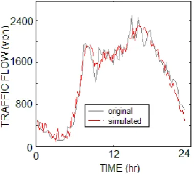
[image:5.595.91.281.147.318.2]In figure 7, the original traffic flow data on any arbitrary day is plotted and compared with the simulation obtained from the model developed in the paper.
Figure 7:Original observations along with simulated data
The root mean square error (RMSE) is around 152 and the mean absolute percentage error (MAPE) is 16.5%. The inclusion of the simplest time-series model reduces the error nearly by approximately 5% from the one mentioned in section IIIc. The MAPE value obtained from a SARIMA (seasonal autoregressive integrated moving average) model [9] is nearly 11%. The model developed in the paper is useful in identifying a trend using a nonfunctional form and does not require data from the recent past.
V CONCLUSION
The methodology in this paper develops a realistic trend based simplistic traffic flow model which can work effectively in the areas where continuous data is not collected over a long period of time. The wavelet analysis based model is parsimonious and does not need any transformation to model non-stationary traffic flow data like time-series techniques. It is flexible compared to other existing models as trend is represented by non-analytic functions using wavelet analysis. Further it has the ability to compress data and represent the random fluctuation optimally using simple time series models with acceptable accuracy. The current model developed here does not depend solely on the current traffic situation to predict in near or distant future. Future work in developing multi-scale time-series models for the detail coefficients of the traffic flow can follow from the current study.
VI REFERENCES
[1]. B. Van Arem, H.R. Kirby, M.J.M. Van Der Vlist, and J.C. Whittaker, “Recent advances and applications in the field of short-term traffic forecasting” International Journal of Forecasting, vol. 13, pp. 1-12, 1997. [2]. E.I. Vlahogianni, J.C. Golias and
M.G. Karlaftis, “Short-term forecasting: Overview of objectives and methods”, Transport Reviews, vol. 24 issue 5, pp. 533-557, 2004. [3]. G. Davis and N. Nihan,
“Nonparametric Regression and Short-Term Freeway Traffic Forecasting”, Journal of Transportation Engineering, vol. 117, pp. 178-188, 1991.
[4]. B.L. Smith, M.J. Demetsky, “Short-term traffic flow prediction: neural network approach”, Transportation Research Record 1453, pp. 98–104, 1994.
[5]. B. L. Smith and M. J. Demetsky, “Traffic flow forecasting: comparison of modelling approaches”, Journal of Transportation Engineering, vol. 123 issue 4, pp. 261–266, 1997.
[6]. B.M. Williams, and L.A. Hoel, “Modelling and forecasting vehicular traffic flow as a seasonal ARIMA process: Theoretical Basis and Empirical Results”. Journal of Transportation Engineering, vol. 129 issue 6, pp. 664-672, 2003.
[7]. H. Sun, H. Xiao, F. Yang, B., Ran Y. Tao and Y. Oh, “Wavelet preprocessing for local linear traffic prediction”, Presented at the 85th
Annual Meeting of Transportation Research Board, Washington, D. C., 2005.
[8]. G. Mao, “A Timescale Decomposition Approach to Network Traffic Prediction”, IEICE Transactions Communication, vol. E88–B, issue 10, pp. 3974-3981, October 2005.
[9]. B. Ghosh, B. Basu, and M.M. O’Mahony, “Time-series modelling for forecasting vehicular traffic flow in Dublin”, Presented at the 85th