Munich Personal RePEc Archive
An Over-the-Counter Approach to the
FOREX Market
Geromichalos, Athanasios and Jung, Kuk Mo
2015
Online at
https://mpra.ub.uni-muenchen.de/64402/
An Over-the-Counter Approach to the FOREX Market
Athanasios Geromichalos
University of California - Davis
Kuk Mo Jung
Henan University
This Version: January 2015
ABSTRACT ————————————————————————————————————
The FOREX market is an over-the-counter market (in fact, the largest in the world) character-ized by bilateral trade, intermediation, and significant bid-ask spreads. The existing interna-tional macroeconomics literature has failed to account for these stylized facts largely due to the fact that it models the FOREX as a standard Walrasian market, therefore overlooking some important institutional details of this market. In this paper, we build on recent developments in monetary theory and finance to construct a dynamic general equilibrium model of interme-diation in the FOREX market. A key concept in our approach is that immediate trade between ultimate buyers and sellers of foreign currencies is obstructed by search frictions (e.g., due to geographic dispersion). We use our framework to compute standard measures of FOREX mar-ket liquidity, such as bid-ask spreads and trade volume, and to study how these measures are affected both by macroeconomic fundamentals and the FOREX market microstructure. We also show that the FOREX market microstructure critically affects the volume of international trade and, consequently, welfare. Hence, our paper highlights that modeling the FOREX as a friction-less Walrasian market isnotwithout loss of generality.
—————————————————————————————————————————-JEL Classification: D4, E31, E52, F31
Keywords: FOREX market, over-the-counter markets, search frictions, bargaining, monetary-search models
Email: [email protected], [email protected].
1
Introduction
The foreign exchange (FOREX) market is an institution of paramount importance since it consti-tutes the channel through which international liquidity is allocated, thus assisting international trade and investment. Moreover, the FOREX market is an over-the-counter (OTC) market, in fact, the largest in the world, characterized by bilateral trade, intermediation, and bid-ask spreads (see Lyons (2001) and?). The traditional international macroeconomics literature has failed to account for these characteristics largely due to the fact that it models the FOREX as a standard, frictionless Walrasian market, therefore overlooking some important institutional details of this market. To remedy this deficiency we build on recent developments in monetary theory and finance to construct a dynamic general equilibrium model of intermediation in the FOREX market. We use this framework to compute explicitly standard measures of FOREX market liquidity, such as bid-ask spreads and trade volume, and to study how these measures are affected both by monetary policy and the FOREX market microstructure. Our model offers new and important insights in comparison to the conventional approach, since it allows us to examine how the FOREX trading frictions affect the volume of international trade and, conse-quently, welfare.
To motivate our story, consider an agent who resides in countryAand wishes to acquire cur-rency of countryB(e.g., in order to purchase some goods or services from a firm in that country, buy some assets in that country, or go on vacation to that country). At the same time, an agent who resides in country B might wish to acquire currency of countryA for similar reasons. If these two agents could contact each other, they might be able to carry out a mutually beneficial currency trade.1 However, an immediate contact between the two agents might be difficult:
the environment described here is clearly characterized bysearch frictions. If there exists a third party who can bypass these frictions, then intermediation services will arise naturally. This idea, which can be traced back to Rubinstein and Wolinsky (1987), seems especially relevant within the context of the FOREX market, given the difficulty of immediate trade among (ulti-mate) buyers and sellers of foreign currencies (e.g., due to geographic dispersion).
To formalize this idea, we develop a two-country, two-currency monetary-search model based on Lagos and Wright (2005) (henceforth, LW). Due to frictions, such as anonymity and limited commitment, trade of home goods in each country necessitates the use of local cur-rency.2 Agents work in their home country and receive local currency which they use to
pur-chase home goods, but they can also exchange for foreign currency in the FOREX market,
1This argument implicitly assumes the absence of a global centralized market for currencies, which is the case
in practice. In this paper, we remain agnostic as to why such a market does not exist, and choose to model the FOREX market in an empirically relevant way, i.e., as a decentralized OTC market.
2Strictly speaking, these frictions make the use of a medium of exchange necessary, and agents are free to carry
should an opportunity to consume abroad arise. We model the FOREX market as an OTC mar-ket following the influential work of Duffie, Gˆarleanu, and Pedersen (2005) (henceforth, DGP). In this market, agents who wish to acquire foreign currency meet with FOREX intermediators or dealers in a bilateral fashion and privately negotiate over the terms of trade. A key feature of the model is that FOREX dealers can participate in a well-networked interdealer market, which guarantees access to a large pool of agents (i.e., traders represented by other dealers) who offer what their clients are searching for, namely, foreign currency. The unique ability of dealers to access this frictionless market is precisely what allows them to bypass the search frictions that obstruct direct trade among agents, and, hence, charge positive bid-ask spreads.
The model delivers closed form solutions for the dealers’ bid and ask prices, and allows us to study how the spread is affected both by market microstructure (e.g., dealer availability and agents’ bargaining positions), and by macroeconomic fundamentals (e.g., inflation). We find that the spread is negatively related to dealer availability. A lower ex ante likelihood of con-tacting a dealer discourages agents from carrying large amounts of real home money balances (which is costly), thus, making them more liquidity constrained and increasing their marginal benefit from consuming foreign goods. As a result, these agents are willing to give up more units of home currency in exchange for one unit of foreign currency, which allows dealers to extract higher fees. Since the ease with which agents can contact a dealer is typically interpreted as a measure of market liquidity, this result implies that bid-ask spreads will be tighter in more liquid markets, a finding which is well-established both in the theoretical and the empirical fi-nance literature (e.g., see DGP and the references therein). However, the channel through which this result emerges in our framework is quite different. For instance, in DGP, a higher probabil-ity of contacting a dealer effectively increases the agent’s bargaining power (and tightens the spread) by making access to alternative trading partners easier. In our paper, a higher probabil-ity of contacting a dealer effectively increases the agent’s bargaining power by making her less liquidity constraint, and, thus, less eager to acquire foreign currency in the FOREX market.
We also find that the bid-ask spread is increasing in the dealers’ bargaining power. An in-crease in the dealers’ bargaining power induces agents to carry a larger amount of real home money balances into the FOREX market, because they realize that they will now need to give up more units of home currency to acquire one unit of foreign currency. As we have already seen, this tends to make agents less liquidity constrained, and effectively improve their bargaining position. However, while the typical agent carries more (real) home currency, a disproportion-ately large fraction of this currency is collected by the dealer as a fee, and, ultimdisproportion-ately, the net effect on the bid-ask spread is positive.
consum-ing foreign goods. Put simply, a high rate of inflation in the home country makes agents more desperate for the foreign good and, hence, the foreign currency, and effectively worsens their bargaining position allowing dealers to extract higher fees.
Our model also has interesting implications for the FOREX trade volume. We character-ize trade volume at both layers of the FOREX market, i.e., agent-dealer and interdealer trade, and we find a positive correlation between dealer availability and trade volume at both levels. Like before, an increase in the ex ante likelihood of contacting a dealer raises the amount of real home money balances that agents bring into the FOREX market. As a result, in any given agent-dealer meeting, a larger volume of currencies change hands, but, moreover, dealers (who represent agents who now have a higher demand for foreign currency) place larger orders for foreign currencies in the interdealer market. Except from thisindirectpositive effect on the in-tensive margin, an increase in dealer availability alsodirectlyincreases the extensive margin of agent-dealer trade volume, since it implies a higher number of agent-dealer matches.
Interestingly, changes in the dealers’ bargaining position affect the volume at the two layers of FOREX trade differently. For instance, consider an increase in the dealers’ bargaining power, which, as we saw, induces agents to carry more real home money balances into the FOREX mar-ket. Since an even larger fraction of the (higher) real balances is now reaped by the dealers, the effect of such change on the agent-dealer trade volume is undoubtedly positive. However, since a large fraction of real balances ends up directly in the dealers’ pockets as a fee, the amount of currencies that get re-shuffled through the interdealer market, i.e., the interdealer trade volume, decreases. Finally, we show that a higher inflation in either country lowers the trade volume at both layers of FOREX trade through the usual negative effect on real balances.
1.1
Related Literature
After the collapse of the Bretton Woods System in the early 70s, advanced economies started adopting a floating exchange rate regime, which spurred a large literature on the FOREX rate determination. Some early works include Dornbusch (1976), Lucas (1982), and Meese and Ro-goff (1983). These seminal papers, and the ones inspired by them, are useful to study the effect of macroeconomic fundamentals (e.g., inflation and productivity in each country) on the deter-mination of the FOREX rate. However, the international macroeconomics literature typically models the FOREX market as a perfectly competitive market, therefore overlooking some im-portant institutional details of this market, such as intermediation, spreads, etc.
As a response, a new approach, often referred to as the FOREX microstructure literature, has emerged over the last two decades. Influential works in this dimension of research include Admati and Pfleiderer (1988), Ito, Lyons, and Melvin (1998), Evans and Lyons (2002), and Evans and Lyons (2005). In this literature, the role of intermediation in the FOREX market is explicitly studied, and it arises due to the presence of frictions, such as adverse selection and inventory costs.3 Although the microstructure literature has given us fruitful insights on many aspects
of the FOREX rate determination which had been overlooked by the international macroeco-nomics literature, it has itself neglected the role of macroeconomic fundamentals, which is ar-guably very important for the determination of exchange rates in the long-run.
Our paper can be viewed as an attempt to bridge the gap between the two strands of the literature.4 Modeling the FOREX market as an OTC market within a dynamic general
equilib-rium framework allows us to study questions that neither of the two existing approaches can study in isolation. For instance, our model can be used to examine the effect of monetary pol-icy on standard measures of FOREX market liquidity, such as bid-ask spreads. This would not be possible within the international macroeconomics literature, because, as is well-known, in a Walrasian market there is no room for intermediation and spreads. Also, studying this ques-tion would not be possible within the microstructure literature, because the majority of these papers adopt a partial equilibrium approach, where foreign currency is not explicitly modeled as money whose holding cost is controlled by monetary policy. Similarly, our paper offers a framework for studying how the FOREX market microstructure can affect international trade and welfare, which would not be possible within either of the existing strands of the literature. In addition, our search-based approach to modeling intermediation in the FOREX market sets this paper aside from the microstructure literature, where intermediation typically arises
3The first is based on the idea that some information relevant to exchange rates is not publicly available. In
the presence of asymmetric information, intermediaries can arise and charge bid-ask spreads due to their ability to buffer against adverse selection (for example, see Copeland and Galai (1983), Glosten and Milgrom (1985) and Kyle (1985)). The inventory cost based models revolve around the idea that intermediaries can provide immediacy (i.e., guarantee of fast service) in an environment where holding positive inventories is costly (for example, see Amihud and Mendelson (1980) and Ho and Stoll (1981)).
4Lyons (2001) estimates that “the uneasy dichotomy between macro and micro approaches is destined to fade”.
due to the existence of adverse selection or inventory costs.5 Although these frictions seem
relevant within the context of the FOREX market, we believe that the search frictions approach is also extremely relevant, given the inherent difficulty of immediate trade among buyers and sellers of foreign currencies, mainly, but not exclusively, due to the geographic dispersion of these agents (see Section2.1 for a more detailed discussion). Hence, it is somewhat surprising that this simple idea has not been formally described in the FOREX market literature before.
Methodologically our paper is closely related to Lagos and Zhang (2014), who also develop a monetary-search model augmented to include OTC financial trade, and use it to study the effect of monetary policy on asset prices and the OTC market liquidity. Our model extends this framework to an open-economy setting in order to specifically study the performance of the FOREX market, and how it affects international trade and welfare. Geromichalos and Herren-brueck (2012) consider a model where agents can allocate their wealth between money and an illiquid asset, and, following an idiosyncratic consumption shock, they can acquire additional liquidity in an OTC financial market. The present paper has similar structure since agents who get an opportunity to consume abroad can acquire foreign currency in the OTC FOREX market. Our paper is also related to Trejos and Wright (2012), who develop a framework that nests the DGP model into a “second-generation” monetary-search model (e.g. Shi (1995) and Trejos and Wright (1995)) and discuss similarities and differences between the two literatures.
The present paper is closely related to a number of works that employ monetary-search models to address long-standing questions in international macroeconomics. For instance, Mat-suyama, Kiyotaki, and Matsui (1993) develop a two-country search model and study the condi-tions under which the two currencies arise as media of exchange in different countries. Wright and Trejos (2001) study the same question, but they employ a second generation monetary-search model where prices are endogenized using bargaining theory. Head and Shi (2003) de-velop a two-country model and show that the nominal exchange rate depends on the stocks and growth rates of the two monies. More recently, Geromichalos and Simonovska (2014) build a two-country model where assets can help agents facilitate international transactions, and use it to rationalize the well-known asset home bias puzzle. Zhang (2014) develops an information-based theory of international currency, and shows that the threat of losing international status imposes an inflation discipline on the issuing country. Finally, Bignon, Breton, and Rojas Breu (2013) build a two-country model of currency and endogenous default to study whether im-pediments to credit market integration can affect the desirability of a currency union.6
The remainder of the paper proceeds as follows. Section 2describes the physical environ-ment and the salient features of the FOREX market that our model aims to capture. Section 3 studies the agents’ optimal behavior. Section4 defines a stationary equilibrium in the
two-5In that respect, our theory of intermediation is closer to Shevchenko (2004) and Wright and Wong (2014). 6 Jung and Pyun (2015) and Jung and Lee (2015) also study how liquidity premia of assets can rationalize other
country model, and describes how the key variables are affected by changes in macroeconomic fundamentals and the FOREX market microstructure. Section5concludes.
2
Physical Environment
Time is infinite and discrete. There are two countries,AandB. Each country has a unit measure of buyers, and sellers with a measure equal to1 +δ,δ ∈[0,1]. The identity of buyers and sellers is fixed over time. We will use the terms “buyer (seller) from countryi” and “buyer (seller)i” interchangeably. There exists a third type of agents calleddealerswith a measure ofv. Dealers have no national identity. All agents are infinitely lived and discount future at rateβ ∈ (0,1). Three divisible and non-storable consumption goods are produced and traded: a general good produced by all agents and a special goodiproduced only by sellers in each countryi∈ {A, B}. Each country’s monetary authority issues a perfectly divisible and storable fiat currency, which we will refer to as moneyi, i ∈ {A, B}. Let Ami,t denote the stock of moneyi at time t. The money stock is initially given byAmi,0 ∈ R++, and thereafter it grows at a constant rate γi (i.e.,
Ami,t+1 =γiAmi,t), whereγi ≥ βis chosen by the monetary authority in countryi. Newmoneyi is introduced (ifγi >1) or withdrawn (ifγi <1) via lump-sum transfers to buyers of countryi at the end of every period.
Each period is divided into three subperiods characterized by different economic activities. We begin with an intuitive description of the environment. A formal decription of each subpe-riod will follow. In the third subpesubpe-riod, agents trade in perfectly competitive or Walrasian mar-kets. This subperiod can be thought of as the settlement stage, where agents from each country work and choose a portfolio of (local) money holdings to bring with them in the following period. In the second subperiod, trade takes place in decentralized markets characterized by anonymity and imperfect credit. Due to these frictions, trade in this subperiod necessitates the use of a medium of exchange (MOE). Agents who wish to acquire foreign currency, in order to purchase foreign goods during the round of decentralized trade, can do so in the FOREX mar-ket which opens in the first subperiod of each period. Hence, the FOREX marmar-ket is strategically placed before the decentralized goods markets open, but after agents have found out whether they have an opportunity to consume the foreign (special) good in the current period.
We now proceed to a formal description of the subperiods, starting with the third one and moving backwards. In the third subperiod, all agents have access to a technology that allows them to transform a unit of labor into a unit of general good. Buyers and sellers from country
end of the third subperiod, a fractionδ∈ [0,1]of buyers obtain an opportunity to consume the foreign special good in the forthcoming period. These buyers are referred to as the C-types, and the rest are referred to as the N-types.All buyersget to consume the local special good.
In the second subperiod, a distinct decentralized market opens in each country (henceforth,
DMi). InDMi, local sellers and buyers, who might be locals or foreigners, trade special good
i. Within anyDM, trade is bilateral and anonymous, and buyers cannot commit to repaying their debt. Thus, all trade has to bequid pro quo. When a seller meets a foreign buyer, the buyer can, in principle, pay the seller with a combination of local and foreign currency. However, as we have seen, seller i cannot visit CM−i, and, therefore, she will not accept foreign currency as payment.7 Hence, although we do not make assumptions that explicitly preclude money
−i from serving as a MOE inDMi, it turns out that only local currency will serve as a MOE in each
DM. This implies that C-type buyers−iwho did not acquiremoneyi in the FOREX market (see next paragraph), will not participate inDMi. Thus, in anyDM, the measure of sellers (1 +δ) is weakly greater than the measure of buyers, and we assume that all buyers (i.e., agents on the short side of the market) match with a seller. The probability with which a seller matches with a local or foreign buyer only depends on the relative measures of these two groups. Finally, within any given match, buyers make a take-it-or-leave-it (TIOLI) offer to the seller.
Given the discussion so far, it follows that C-type buyers want to acquire foreign currency beforeDM trade begins. Interestingly, buyers from countryihold precisely what (C-type) buy-ers from country−ineed:moneyi. However, to make things interestingandrealistic, we assume that immediate trade between these agents is impossible. Buyers who wish to acquire foreign currency have to visit the FOREX market which operates in the first subperiod. Following DGP, we model this market as an OTC market characterized by search and bilateral trade between dealers and buyers. LetαD ∈[0,1]denote the probability with which the typical dealer contacts a buyer in the FOREX, so, by symmetry, αD/2 is the probability that this buyer is a citizen of countryi, i ∈ {A, B}. Similarly,αi ∈ [0,1]represents the probability with which buyeri con-tacts a dealer. Within any given buyer-dealer pair, the terms of trade are determined through proportional bargaining (Kalai (1977)), withθ ∈[0,1]denoting the dealer’s bargaining power.
When a dealer meets with a C-type buyer−i she can provide that agent withmoneyi that comes from two potential sources. First, the dealer may carry somemoneyi that she acquired in the precedingCMi(recall that a dealer can visit both CMs). Second, the dealer has immediate access to a perfectly competitiveinterdealer market, where she can acquiremoneyi, at the ongoing market price, from dealers who either contacted buyersior carrymoneyion their own account.
7Given that currencies are fiat, an agent will hold money only for two reasons: i) to use it as a MOE to purchase
special goods in theDM round of trade; or ii) to sell it for the general good in theCM round of trade. Since the identity of agents is fixed, a seller will never hold money in order to use it as a MOE. A seller might be willing to accept money as a MOE in theDM, if she hopes to trade it for some general good in the forthcomingCM. But, by assumption, sellerinever gets to visitCM−i, i.e., the market wheremoney−iis traded for general good. Hence, a
The ability of dealers to access this frictionless market is precisely what allows them to bypass the search frictions that obstruct direct currency trade between buyers.8 This assumption is also
consistent with the fact that, in practice, FOREX dealers have access to a well-networked inter-dealer market. We have now finished describing all three subperiods. The timing of events is summarized in Figure1.
[image:10.612.95.516.152.416.2]1st subperiod 2nd subperiod 3rd subperiod
Figure 1: Timing of trading process
Finally, consider agents’ preferences. The utility of the typical buyeriis given by
E0
∞
X
t=0
βt{u(qt) +u(˜qt) +Xt−Ht},
where qt(q˜t) denotes consumption of the local (foreign) special good in the second subperiod of periodt. The termsXt andHt stand for the consumption of general good and the effort to produce that good in the third subperiod of periodt, respectively.9 We assume thatu(·)is twice
continuously differentiable, withu(0) = 0, u′(·) >0, u′(0) = ∞, u′(∞) = 0, andu′′(·) <0. The
termE0denotes the expectation with respect to the probability measure induced by the random
trading process in theDM s. The utility of the typical selleriis given by
8Assuming that dealers have access to a competitive interdealer market is standard in the recent literature on
OTC financial trade; e.g., see Weill (2011) and Lagos, Rocheteau, and Weill (2011).
9All the results will remain unaltered if one assumes quasi-linear (instead of linear) preferences, as in LW. The
E0
∞
X
t=0
βt{−qt+Xt−Ht},
whereXt, Ht,E0 are as above, and−qtis the disutility of producingqtunits special good in the second subperiod of t (i.e., without loss of generality, we assume that the disutility is linear). Finally, the utility of the typical dealer (who does not participate in the DM) is given by
E0
∞
X
t=0
βt{Xt−Ht},
where all the symbols have already been explained.
2.1
Discussion of the Physical Environment
Since this is (to the best of our knowledge) the first open-economy monetary model that speci-fies the FOREX market explicitly as a decentralized OTC market, some of the model’s assump-tions might appear to be non-standard, and, hence, deserve some discussion.
For instance, we assume that agents from country i cannot visit CM−i, where money−i is traded in a competitive environment.10 This assumption aims to capture the simple and
em-pirically relevant idea that citizens of countryilive and work in their home country, get paid in local currency, and, whenever they have a need to purchase foreign goods, they exchange local for foreign currency within a special institution known as the FOREX market. If agents from countryiwere allowed to acquiremoney−i inCM−i(which, recall, is a perfectly competi-tive market), this would defeat the very purpose of this paper, which is to explicitly model the FOREX as an OTC market characterized by bilateral trade and intermediation.
We have also seen that only moneyi serves as a MOE in DMi. Strictly speaking, this is a result rather than an assumption of the model, and it follows directly from the assumption that sellersicannot visitCM−i (see footnote7), which, in turn, is adopted for the reasons described in the previous paragraph. However, we do not claim that our paper offers a “deep” theory of which assets serve as MOE in various types of international meetings, because this is not the question that we are after. Zhang (2014) asks precisely this question (among others) and shows that, if sellers must pay a relatively high cost to verify the genuineness of foreign currency (an assumption which is quite reasonable), then a “local currency dominance” equilibrium, where
moneyi serves exclusively as a MOE inDMi, will ariseendogenously.
In our model, intermediation in the FOREX market arises because direct currency trade be-tween buyers from the two countries is difficult. One can think of buyerias a Swiss importer
10This assumption is new even within the class of models that employ two-country versions of LW. For instance,
Geromichalos and Simonovska (2014) interpretCMi as an analogue ofE-trade, where agents from all over the
of US computers, and buyer−ias an American importer of Swiss chocolate. Since the former agent wishes to transform Swiss francs into dollars and the latter wishes to purchase Swiss francs with her dollars, it seems like the two agents could carry out a mutually beneficial cur-rency trade. However, contacting each other and carrying out this trade is clearly difficult for the two buyers in our example.11 In this environment, the buyers are happy to purchase foreign
currency from FOREX dealers, and the dealers can charge an intermediation fee which reflects their ability to access a well-networked (and practically competitive) interdealer market, and, hence, bypass the frictions that prevent direct trade between currency buyers.12
This discussion clarifies that the search frictions, which play a central role in our analysis, refer to the difficulty of agentito contact agent−iand purchase foreign currency directly from her, and not (necessarily) to the difficulty of agentito contact a dealer. The latter is simply cap-tured by the parameterαi ∈ [0,1]. Thus, if a buyer of currency can find a dealer fairly quickly, in the context of our model, this would imply a large value ofαi.13 It is also important to clarify that trade among dealers is not characterized by any frictions whatsoever (dealers trade with each other in a perfectly competitive interdealer market). This is precisely why our model pre-dicts the existence of positive bid-ask spreads in dealer-customer transactions, but no spreads in interdealer transactions, which is consistent with the empirical observation (for instance, see Lyons (2001)).
To conclude this section, we briefly discuss how two of the most important parameters of the model, namely αi and θ, map into the real-world FOREX market. As we have already described, αi captures the degree of dealer availability in that market. Therefore, one can in-terpret the recent emergence of many online FOREX dealers and multilateral trading facilities (MTFs) as an increase in αi.14 The term θ stands for the bargaining power of the dealers in a typical buyer-dealer match. Hence, generally speaking, this parameter reflects the negotiating strength of the dealers, but, more specifically, it can be thought of as a shortcut for capturing certain market conditions which we have not explicitly modeled. For instance, in our model the
11Even if the search frictionper seis not immense enough to preclude contact between the two parties, there
are other reasons, such as the asymmetric demand for foreign currencies, that can render such trade difficult. For instance, even if it is relatively easy for the two buyers to contact each other, say, through the internet, it might still be the case that the Swiss importer of computers seeks to purchase 10 million US dollars, while the American importer of chocolate only wants to convert 100,000 USD into Swiss francs. In this case, the Swiss importer would have to search for multiple trading partners, which would make the overall transaction complicated.
12Here, for the sake of simplicity, we have assumed that currency trade between buyers from the two countries
isimpossible. However, all one needs to assume in order to generate a role for intermediation in the FOREX market, is that direct trade between these agents is (just)difficult. For instance, one could assume that the C-type buyeri
first attempts to trade directly with buyer−i, and then, if that attempt proves unsuccessful, she resorts to dealers’ services. This alternative specification would make the analysis more cumbersome, but it would not add any interesting insights to the model.
13In fact, most of the results of the paper would remain valid even in the extreme case withα
i = 1. This is true
because settingαi = 1does not imply that we are in a “frictionless” environment, since, as we just explained, the
friction here concerns the difficulty to buy currency directly from foreign agents and not the availability of dealers.
14Examples of such online dealers include FXall, Atriax, FXchange, FXconnect, FXtrade, Gain.com,
measure of dealers is fixed, however, θ may capture the degree of competition for customers among dealers (i.e., a low θ can be interpreted as a market where many dealers compete for few currency customers). Similarly, in our model we have excluded direct currency trade be-tween buyers from different countries (see footnote12), however, θmay capture the degree to which it is possible for buyer ito contact (and directly trade with) buyer −i(i.e., a high θ can be interpreted as a market where direct trade between ultimate buyers and sellers of currency is extremely difficult).
3
Value Functions and Optimal Behavior
3.1
Value Functions
Consider first the typical buyer i, who enters CMi with mi units of home currency. For this agent, the Bellman’s equation satisfies15
WB
i (mi) = max X,H,mbi
X−H+βEk{Ωki(mbi)}
s.t. X+ϕimbi =H+ϕimi+Ti,
where variables with a hat indicate next period’s choices. The term ϕi denotes the price of
moneyiin terms of the general good, andTiis the real value of the lump-sum monetary transfer by the monetary authority of country i. The function Ωk
i represents the value function in the FOREX market for a buyer of typek =C, N. EliminatingHfrom the budget constraint yields
WiB(mi) =WiB(0) +ϕimi, (1)
WB
i (0) ≡Ti+ max
b
mi
−ϕimbi +βEk{Ωik(mbi)} , k ∈ {C, N}.
As is standard in models that build on LW, the buyer’s value function is linear in the money holdings, implying that there are no wealth effects on the choice ofmbi.
Next, consider the CM value function for the typical seller i. This agent will never want
15 A buyer who acquired some foreign currency in the FOREX market of periodt, may fear that she might not
be able to trade again in that market int+ 1(given the search frictions). Hence, she might choose to not spend all of her foreign currency in theDM of periodt, but instead keep some to trade in theDM oft+ 1. The problem with this type of strategy is that, if buyers (in periodt) can keep some foreign currency to trade in theDM of
t+ 1, they can do the same for theDM oft+ 2, t+ 3, and so on. Allowing this type of strategy would make the model intractable. Hence, we require that buyers spend all the foreign currency acquired in the FOREX market of periodtin theDMof that period. This implies that as these agents enter their homeCMthey can only hold home currency. Although here, for the sake of simplicity, we assume that buyersmustspend all their foreign currency in the currentDM, as long as the probability of meeting a dealer,αi, is large enough, buyers will actuallychooseto
to leave the CM with any money holdings, since she does not want to consume in the DM
round of trade (see Rocheteau and Wright (2005) for a rigorous proof). The seller will typically hold some home currency, which she received as payment (either from a local or from a foreign buyer) in theDM. For this agent, the Bellman’s equation satisfies
WS
i (mi) = max X,H
X−H+βVS i (0)
s.t. X =H+ϕimi,
where VS
i (0) denotes the seller’s value function in DMi. Replacing H from the budget con-straint intoWS
i yields
WS
i (mi) = βViS(0) +ϕimi.
A dealer is the only type of agent who might enter the third subperiod with a portfolio that contains both currencies,m≡(mA, mB). For this agent, the Bellman’s equation satisfies
WD(m) = max X,H,mb
{X−H+βΩD(mb)}
s.t. X+ϕmb =H+ϕm,
whereΩD(mb)denotes value function of a dealer who enters the FOREX market with portfolio
b
m. Also, we defineϕ ≡(ϕA, ϕB), and we letϕmdenote the dot product ofϕandm.
Eliminat-ingH from the budget constraint implies that
WD(m) = WD(0) +
ϕm, (2)
WD(0)≡max
b
m
{−ϕmb +βΩD(mb)}.
Before we proceed to the description of the FOREX market value functions, we introduce two useful definitions. First, letWfD(m)denote the continuation value of a dealer who just (op-timally) rebalanced her portfolio,m, in the interdealer FOREX market. This function satisfies
f
WD(m) = max
e
m
WD(
e
m) (3)
s.t. meA+εmeB ≤mA+εmB,
whereme ≡ (meA,meB)denotes the post-interdealer market portfolio of the dealer, and the
con-straint requires that the value of the post-interdealer market portfolio (measured in terms of
Second, consider a meeting between a dealer who enters the FOREX market with portfolio
mdand a buyer from countryiwho carriesmi units of home currency. Then, the terms
¯
miA(mi, ε,ϕ),m¯iB(mi, ε,ϕ),
¯
mdA m d
, mi, ε,ϕ
,m¯dB m d
, mi, ε,ϕ
denote the portfolios that the buyer and the dealer (respectively) hold after all FOREX trading has concluded (i.e., it includes the buyer-dealer trade and the interdealer market trade).16
Now consider the expected FOREX value function for the tyipcal buyer i who enters the first subperiod withmi units of home currency. This functions satisfies
Ek{Ωki(mi)}=δΩCi (mi) + (1−δ)Vin(mi), (4)
whereΩC
i (mi)denotes the FOREX value function for a buyeriwho gets to consume the foreign special good in the forthcoming DM−i, and Vin(mi) denotes the value function for a buyer i who proceeds toDMi with her original (home) money holdings. Furthermore, we have
ΩCi (mi) =αiV y i m¯
i A,m¯
i B
+ (1−αi)Vin(mi), (5)
whereVn
i has been explained earlier, andV y
i ( ¯miA,m¯iB)denotes theDM value function for buyer
i, conditional on having met with a dealer in the preceding FOREX market.
The value fuunction for a dealer who enters the FOREX market with portfoliomdsatisfies17
ΩD(md) =(1−αD)WfD(md) (6)
+ αD 2
Z f
WD m¯d
A m
d, m
A, ε,ϕ,m¯dB md, mA, ε,ϕdFA(mA) + αD
2
Z f
WD m¯d
A m
d, m
B, ε,ϕ,m¯dB md, mB, ε,ϕdFB(mB),
whereFiis the cumulative distribution function over themoney
iholdings of the random buyer
iwhom the dealer may contact in the FOREX market.
Finally, consider the value functions in theDM round. For a C-type buyeriwho matched
16The exact solutions for the post-trade portfolios will be rigorously analyzed in Section3.2. For now, we use
the termsm¯i
Aandm¯iA(mi, ε,ϕ), orm¯dAandm¯dA md, mi, ε,ϕ, etc., interchangeably.
17As we have already explained, the variousWfDterms denote the continuation value for a dealer who
rebal-ances her portfolio in the interdealer FOREX market. However, the composition of that portfolio critically depends on whether the dealer matched with a buyer, and, if yes, on the buyer’s citizenship and her money holdings. So, for example, the first line on the RHS of eq.(6) describes the event in which the dealer does not contact any buyer and proceeds to the interdealer market with her original portfolio,md. The second line describes the event in
which the dealer contacts a buyer from country A, in which case she proceeds to the interdealer market with portfolio( ¯md
with a dealer in the preceding FOREX market and carries a portfolio(mA, mB), we have18
Viy(mA, mB) = u(q) +u(˜q) +WiB(mi−p), (7)
whereq (q˜) denotes the consumption of local (foreign) special good, andpthe units ofmoneyi that the buyer transfers to selleriinDMi. These terms will be determined in Section3.2. Fur-thermore, for the typical buyeriwho only participates in her homeDM (either because she is an N-type or because she did not contact a dealer in the FOREX market), we have
Vin(mi) =u(q) +WiB(mi−p). (8)
TheDM value function for selleri, who entersDMiwith no money, is given by
VS
i =
1 1 +δ
−q+WS i (p)
+ δα−i 1 +δ
−q˜+WS i (˜p)
+ δ(1−α−i)
1 +δ W
S
i (0), (9)
whereq, pdenote the production of special good, and the units ofmoneyiexchanged in a meet-ing with a local buyer, andq,˜ p˜are the analogue expressions for a meeting with a foreign buyer. The expressionδ(1−α−i)/(1 +δ)in the third term on the RHS of eq.(9) is the probability with which the seller does not match with a buyer, in which case she proceeds toCMiwith no money.
3.2
Terms of Trade
In this section, we study the determination of the terms of trade in the various markets. First, consider a meeting inDMibetween a selleriand a buyeri(a local) who carriesmiunits of local currency. The two parties negotiate over a quantity of special good, q, to be produced, and an amount ofmoneyi, p, to be delivered to the seller. Given that the buyer makes a TIOLI offer to the seller, the bargaining problem can be expressed as19
max
p,q {u(q) +W
B
i (mi−p)−WiB(mi)}
s.t. q =WiS(p)−WiS(0),
18As we have already argued, the buyer will spend all her foreign currency inDM
−i, hence, the only argument
insideWB
i is home money holdings.
19At this stage the buyer has already made her portfolio decisions (i.e., how much home currency to keep and
and the feasibility constraintp≤mi. Given the linearity ofWiB, WiS, the problem simplifies to
max
p,q {u(q)−ϕip}
s.t. q =ϕip,
andp≤mi. The next lemma describes the solution to this bargaining problem.
Lemma 1. Defineq∗ ={q:u′(q) = 1}andm∗
i =q∗/ϕi. Then, in aDMimeeting between a selleriand
a local buyer, the bargaining solution is given byq(mi) = min{ϕimi, q∗}andp(mi) = min{mi, m∗i}.
Proof. The proof is obvious, and it is, therefore, omitted.
The interpretation of Lemma 1is standard. The terms of trade, (q, p), depend only on the buyer’s moneyi holdings. Whenmi exceeds a certain level, m∗i, the buyer purchases the first-best quantity,q∗, and gives up exactlym∗
i units ofmoneyi. On the other hand, ifmi falls short ofm∗
i, the buyer is liquidity constrained. In this case, she gives up all hermoneyi, and receives the amount of good that the seller is willing to produce for that money, i.e.,q=ϕimi.
Next, consider a DMi meeting between a seller i and a buyer−i(a foreigner) who carries
mi units ofmoneyi (which to her is foreign currency acquired in the preceding FOREX market). The two parties negotiate over a quantity of special good,q˜, to be produced, and an amount of
moneyi, p˜, to be delivered to the seller. In this type of meeting, the determination of the terms of trade is even more straightforward than before, because the buyer spends all hermoneyi by assumption (see footnote15). The solution to this bargaining problem follows trivially.
Lemma 2. In aDMimeeting between a selleriand a foreign buyer, the bargaining solution is given by ˜
q(mi) =ϕimi andp˜(mi) = mi.
We now proceed to the characterization of the terms of trade in the FOREX market. Consider first a dealer who enters the FOREX market with a portfolio md and does not match with a
buyer. This dealer can still participate in the interdealer market and potentially sell her money to dealers who want to acquire it (e.g., because they matched with C-type buyers). The next lemma describes the continuation value of this agent.
Lemma 3. A dealer who enters the first sub-period with portfoliomd, and does not contact any buyer,
enters the third sub-period with portfoliomed≡ medA md, ε,ϕ,medB md, ε,ϕ, given by
e
mdA=
0, if εϕA < ϕB,
∈[0, md
A+εmdB], if εϕA=ϕB,
md
A+εmdB, if εϕA> ϕB.
e
mdB =
md
B+mdA/ε, if εϕA < ϕB,
md
Moreover, the dealer’s maximum expected discounted payoff is
f
WD(md) = ¯ϕ mdA+εmdB+WD(0), (10)
whereϕ¯≡max{ϕA, ϕB/ε}.
Proof. See the appendix.
Lemma 3 admits an intuitive interpretation. If εϕA < ϕB, then a dealer who holds any
moneyAin the interdealer FOREX market can use a unit ofmoneyAto buy1/εunits ofmoneyB. The net return of this trading strategy isϕB/ε−ϕA, which is strictly positive. Therefore, under these prices, the typical dealer will sell all her moneyA formoneyB in the interdealer market. The same intuition applies to the complementary case (i.e., whenεϕA > ϕB). WhenεϕA =ϕB, the dealer is indifferent with respect to the composition of her portfolio (betweenmoneyA and
moneyB). As we shall see later, this case is the only one that can arise in equilibrium.
We now study the bargaining outcome in a meeting between a C-type buyeriand a dealer in the FOREX market. Since the buyer has an opportunity to consume special good inDM−i, she may want to exchange some of her moneyi formoney−i. In turn, dealers, have the unique ability to access the frictionless interdealer market, where they can acquiremoney−ifrom other dealers, who either contacted buyers from country−ior carry money−i on their own account. Hence, in this type of bilateral meeting there are clear gains from trade, and the two parties will split the surplus according to Kalai’s proportional bargaining solution (withθ ∈(0,1)being the dealer’s bargaining power).20 The bargaining problem is given by
max
¯
md A,m¯
d B,m¯
i A,m¯
i B≥0
n f
WD( ¯md)−fWD(md)o
s.t. 1. θ
1−θ =
f
WD( ¯md)−WfD(md)
Viy( ¯mi)−Vin(mii)
,
2. m¯d A+ ¯m
i
A+ε[ ¯m d B+ ¯m
i B]≤m
d
A+m
i
AI{i=A}+ε
md
B+m
i
BI{i=B}
,
where m¯d ≡ m¯dA,m¯dB,m¯i ≡ ( ¯miA,m¯iB) denote the post-FOREX trade portfolio for the dealer
and the buyer, respectively, andI{i=n}, n∈ {A, B}, is an indicator function that equals 1 ifi=n.
As is standard with proportional bargaining, the problem above maximizes the dealer’s surplus (i.e., her post-negotiation continuation value net of her threat point), subject to two constraints. The first is the so-calledKalaiconstraint, which requires the dealer-to-buyer surplus ratio to equal the ratio of the two players’ bargaining powers (i.e., θ/(1−θ)). The second is the feasibility constraint which requires that the combined value of the pre-trade portfolios is
20For a discussion on the benefits of using Kalai’s (1977) over Nash Jr’s (1950) bargaining solution in monetary
enough to finance the combined value of the post-trade portfolios in the interdealer market. Exploiting the linearity of the value functions the problem simplifies to
max
¯
md A,m¯
d B,m¯
i A,m¯
i B≥0
¯
ϕm¯dA+εm¯ d
B−(m
d
A+εm
d B)
st. 1. θ
1−θ =
¯
ϕm¯d A+εm¯
d
B−(m
d
A+εm
d B)
u(q( ¯mi
i)) +u q˜ m¯i−i
−u(q(mi
i)) +ϕi[p(mii)−p( ¯mii)−(mii−m¯ii)]
,
2. m¯dA+ ¯m i
A+ε[ ¯m d B+ ¯m
i B]≤m
d
A+m
i
AI{i=A}+ε
mdB+m i
BI{i=B}
.
The solution to this bargaining problem is described in the following lemma.
Lemma 4. Consider the bargaining problem between a buyeriand a dealer, who enter the first subperiod with portfoliosmi
i andmd, respectively. Moreover, define the following objects:
χ∗ −i ≡
χ−i :u′(ϕ−iχ−i) =
(ϕAε)I{i=A}+ϕBI{i=B}
ϕBI{i=A} + (ϕAε)I{i=B}
, (11)
G(χ−i)≡
G(χ−i) :
ϕ−iu′(ϕ−iχ−i)
ϕiu′(ϕiG(χ−i))
= ϕ¯I{i=B}+ ¯ϕεI{i=A} ¯
ϕεI{i=B}+ ¯ϕI{i=A}
, (12)
τi(χ−i)≡
θu(ϕ−iχ−i) + (1−θ) ¯ϕχ−i[εI{i=A} +I{i=B}]
θϕi+ (1−θ) ¯ϕ[εI{i=B}+I{i=A}]
. (13)
We have the following results:
a) The buyer’s post-FOREX trade portfolio,m¯i, is given by
¯
mi
−i m i i = χ∗
−i, if mii ≥mi∗+τi(χ∗−i),
{χ−i :mii = Γ (χ−i)}, if mi∗ ≤mii ≤m∗i +τi(χ∗−i),
{χ−i :mii = Λ (χ−i)}, if mii ≤m∗i,
¯
mii m i i = mi
i−τi(χ∗−i), if mii ≥m∗i +τi(χ∗−i),
G m¯i
−i(mii)
, otherwise,
where we have defined
Γ (χ−i)≡G(χ−i) +τi(χ−i) +
θ{u(ϕiG(χ−i))−ϕiG(χ−i)} −θ{u(qi∗)−q∗i}
θϕi+ (1−θ) ¯ϕ[εI{i=B}+I{i=A}]
,
Λ (χ−i)≡G(χ−i) +
θ{u(ϕ−iχ−i) +u(ϕiG(χ−i))−u(ϕimii)}+ (1−θ) ¯ϕχ−i[εI{i=A}+I{i=B}]
(1−θ) ¯ϕ[εI{i=B}+I{i=A}]
.
Also, we haveΓ′(χ
−i)>0,Λ′(χ−i)>0.
b) Define the “ask” and the “bid” price ofmoneyBas follows:
X εa ≡the price ofmoney
X εb ≡the price ofmoney
B in terms ofmoneyAthat a dealer bids to buyerB to buymoneyB.
Then, we haveεa= mAA−m¯ A A
¯
mA B ,ε
b = m¯B A mB
B−m¯ B
B, andε
b ≤ε≤εa.
c) The dealer’s post-FOREX trade portfolio, m¯d A,m¯dB
, is given by
¯
md
A ∈
0, md
A+εm
d
B+
(εa−ε)
I{i=A} +
ε−εb
εb
I{i=B}
¯ mi −i , ¯ md B = 1 ε md
A+εm
d
B+
(εa−ε)
I{i=A}+
ε−εb
εb
I{i=B}
¯
mi
−i−m¯ d A
.
Proof. See the appendix.
The formal proof of the lemma has been relegated to the appendix. Here, we provide an intuitive description of the solution. When buyeri gives up one unit ofmoneyi, this typically reduces the amount of good, sayq, that she can purchase inDMi, but also allows her to acquire
money−i, which she can use to purchase good, say q˜, inDM−i. This transaction will undoubt-edly create a benefit, or surplus, because the buyer’s preferences in the DM round are given byu(q) +u(˜q), withu′ > 0, u′′ <0, andu′(0) = ∞.21 The proportional bargaining solution first
makes sure that the surplus generated by the transaction (i.e., the transfer ofmoney−i to buyer
i) is maximized, and then determines the terms of trade so that the so-called Kalai constraint is satisfied (this last part simply means that the dealer obtains a fractionθof the surplus).
A key observation from Lemma 4 is that the solution to the bargaining problem depends only on the buyer’s pre-trademoneyiholdings,mii. Hence, it turns out that the key contribution of the dealer in this match is her ability to access the interdealer market, and notthe fact that she may be carrying some money on her own account. Technically speaking, this is attributed to the fact that the marginal rate of substitution (MRS) betweenmoneyAandmoneyBfor dealers is exogenously pinned down by the currency prices in the (perfectly competitive) interdealer FOREX market (i.e., the termsε,ϕon the right-hand side of eq.(12)).
Before we explain the solution to the bargaining problem we provide an intuitive interpre-tation of the various terms that appear in Lemma4. The termχ−i stands for the units of foreign currency that buyeriholds after the FOREX meeting, andχ∗
−iis the amount of foreign currency that allows buyerito purchase the first best quantity inDM−i. The termG(χ−i)stands for the post-FOREX amount ofmoneyi held by buyer i, and it is defined in eq.(12), which states that surplus maximization requires that the MRS betweenmoneyi andmoney−i for the buyer (left-hand side of the equation in the curly bracket) should be equal to the MRS betweenmoneyi and
money−i for the dealer (right-hand side of the equation in the curly bracket). The term τi(χ∗−i)
21Hence, ifq˜= 0andq >0, there is always a benefit from reducingqand increasingq˜. In fact, forq˜≈0the
stands for the units of moneyi that the buyer needs to carry in addition tom∗i in order to pur-chase the first best quantity inbothDMs. Naturally, this term is increasing both inχ∗
−i andθ.22 Finally, the terms Γ (χ−i),Λ (χ−i)have been defined such that the equations mii = Γ (χ−i) and
mi
i = Λ (χ−i)represent the Kalai constraint (for different levels ofmii).23
Given this discussion, the interpretation of Lemma 4 becomes quite intuitive. Given her money holdings,mi
i, the buyer can find herself in three possible regions.
1. mi
i ≥m∗i +τi χ∗−i
.
In this region, the buyer’smoneyi holdings are so plentiful that she ends up purchasing the first best quantity in bothDM′s. This requires that the buyer’s post-FOREXmoney
−i holdings equalχ∗
−i, and her post-FOREXmoneyiholdings equal her original holdings,mii, net of the termτi(χ∗−i)described in the previous paragraph.
2. m∗
i ≤mii ≤m∗i +τi(χ∗−i).
In this intermediate region, the buyer can afford to purchaseq∗ in her homeDM but not
in bothDMs. Of course, the buyer could choose to keepm∗
i units ofmoneyi, which would allow her to purchase q∗ inDM
i, but optimality requires that the MRS between moneyi andmoney−i for the buyer should be equal to the MRS between moneyi andmoney−i for the dealer. Put simply, the post-FOREX moneyi and money−i holdings of the buyer are pinned down by eq.(12) and the equationmi
i = Γ (χ−i)(i.e., the Kalai constraint).
3. mi
i ≤m∗i.
In this region, the buyer’s pre-trade money holdings are so scarce that she cannot even afford to purchase q∗ in the homeDM. The interpretation of the bargaining solution is
similar to the one in Region 2: the buyer’s post-FOREXmoneyiandmoney−i holdings are pinned down by eq.(12) and the Kalai constraint. However, given that we are in the case wheremi
i ≤m∗i, the relevant Kalai constraint is now given by the equationmii = Λ (χ−i).
Part (b) of the lemma simply determines the bid and ask price of the dealer (in terms ofmoneyB)
22The more money
−i the buyer wishes to acquire, the more moneyi she should bring. Moreover, whenθ is
higher the transaction fee charged by the dealer is higher, thus, to acquire a given amount ofmoney−ithe buyer
should, on average, bring moremoneyi.
23To see this point, focus on the equationmi
i= Γ (χ−i)(an analogous argument applies to the second equation).
Also, to simplify the illustration here, setεϕA=ϕB(which, of course, will hold in equilibrium, and) which implies
that the termϕ¯[εI{i=B}+I{i=A}], which appears inΓ (χ−i), simplifies toϕi,∀i. Multiply both sides byϕiand solve
with respect toϕimii−ϕiG(χ−i), to obtain
ϕimii−ϕiG(χ−i) =ϕ−iχ−i
+θ{[u(ϕiG(χ−i))−ϕiG(χi)] + [u(ϕ−iχ−i)−ϕ−iχ−i]−[u(q∗)−q∗]}.
This equation states that the dealer should leave the meeting with an amount ofmoneyi(the LHS of the equation)
whose value equals the value of themoney−ithat she brings into the match either through intermediation or on
her own account (the termϕ−iχ−i), plus a fractionθof the surplus generated whenϕ−iχ−i(real) units of foreign
as functions of the post and pre-trade money holdings of buyeri. Part (c) describes the dealer’s post-trade portfolio, which turns out to be indeterminate. This follows from the fact that the dealer can visit both CMs (and sell the currencies for general good), so there is a continuum of portfolio allocations that give her the same payoff. Nevertheless, as the following corollary shows, the combined value of the dealer’s post-trade portfolio is uniquely pinned down.
Corollary 1. ThemoneyAvalue of the dealer’s post-trade portfolio is uniquely given by
¯
md A+εm¯
d
B =m
d
A+εm
d
B+
(εa−ε)
I{i=A}+
ε−εb
εb
I{i=B}
¯
mi
−i.
Corollary1 also clarifies that the dealer extracts a transaction fee from the buyer. For ex-ample, when the dealer encounters a buyerAwho purchasesm¯A
B units of foreign currency, she extracts a total fee equal to (εa−ε) ¯mA
B. Similarly, when the dealer encounters a buyerB who purchasesm¯B
A of foreign currency, she extracts a total fee equal to
(ε−εb)/εbm¯B A.
The following lemma highlights some interesting properties of certain key variables that can be calculated directly from the bargaining solution (Lemma4), such as theaskandbidprice ofmoneyB, and the amount of currency that changes hands. These terms will be crucial for the determination of theequilibriumbid-ask spread and FOREX trade volume later on.
Lemma 5. The Ask and Bid Price satisfy
∂εa
∂θ >0, ∂εb
∂θ <0,
∂εa ∂mA A
= 0, in Region 1,
<0, in Region 2,3,
∂εb ∂mB B
= 0, in Region 1,
>0, in Region 2,3.
The Volume ofmoney−ithe dealer hands over satisfies
∂m¯i
−i
∂θ
= 0, in Region 1,
<0, in Region 2,3,
∂m¯i
−i ∂mi i
= 0, in Region 1,
>0, in Region 2,3.
The Volume ofmoneyithe buyerihands over satisfies
∂(mi i−m¯ii)
∂θ
>0, in Region 1,
>0, in Region 2,3,
∂(mi i−m¯ii)
∂mi i
= 0, in Region 1,
>0, in Region 2,3.
Proof. See the appendix.
the exception of Region 1, where the buyer is not constrained by her home money holdings.24
Naturally, the volume of moneyi that buyeri hands over to the dealer is increasing in θ. The effects of an increase inmi
i work in the opposite way than an increase inθ. An increase in mii typically allows the buyer to purchase more (home and) foreign good, but sinceuis concave, her marginal benefit from acquiring one additional unit of foreign currency, or, equivalently, from consuming one additional unit of foreign good, is diminishing. In a sense, an increase inmi
i makes buyeriless eager to acquire foreign currency, and effectively allows her to obtain better terms of trade in the FOREX market. Finally, with the exception of Region 1, the more
moneyithe buyer carries, the more she hands over to the dealer, due to the fact that the increase inm¯i
−i more than offsets the improvement in the terms of trade, i.e., the decrease inεa.
3.3
Optimal Behavior
In this section, we describe the optimal portfolio choices of buyers and dealers. The first step is to characterize theobjective functionsfor these agents. First, consider the typical dealer. Substi-tute eq.(10) into eq.(6), and lead the emerging expression by one period to obtain
ΩD mbd
=ϕb¯(mbdA+εbmb d
B) +W
D (b0)
+ϕb¯
Z α
D 2 [ε
a(
b
mA)−bε] ¯mAB(mbA)dFA(mbA)
+ϕb¯
Z
αD 2
b
ε−εb(
b
mB)
εb(mb B)
¯
mBA(mbB)dFB(mbB).
Next, substitute ΩD from the last expression into eq.(2), and define the term inside the max operator (i.e., the objective function) asJD. Then, we have
JD mbdA,mb d B
≡ −ϕA+βϕb¯
b
mdA+ −ϕB+βϕb¯εb
b
mdB
+βϕb¯
Z α
D 2 [ε
a(
b
mA)−bε] ¯mAB(mbA)dFA(mbA)
+βϕb¯
Z α
D 2
b
ε−εb(mb B)
εb(mb B)
¯
mB
A(mbB)dFB(mbB).
In the last expression, the fist line represents the cost of carryingmoneyA andmoneyB, the sec-ond line captures the expected discounted benefit from executing buyerA’s order (i.e., purchas-ingmoneyB) in the interdealer market, and the last line admits a similar interpretation (when the dealer meets a buyerB). As we already know from Lemma4, these expected intermediation fees are independent of the dealer’s own portfolio. Also, it is understood that the expressions
24However, for a givenmi
i, increasingθmakes it more likely that the bargaining solution will “fall” in Region 2.
¯
mi
−i, εa,andεb are described by Lemma4.
Next, consider the typical buyer i. Substitute equations (7), (8) into (5), and then plug the emerging expression into eq.(4) and lead it by one period to obtain
Ek{Ωki(mbi)}=ϕbimbi+WiB(b0) +δαi
u q˜i m¯i−i(mbi,bε,ϕb)+u(qi(mbi−ϑ(mbi)))
−δαi[ϕbiϑ(mbi) +ϕbipi(mbi−ϑ(mbi))]
+ (1−δαi){u(qi(mbi)) +ϕbi[mbi−pi(mbi)]},
where ϑ(mbi) represents the units ofmoneyi that buyer ihands over to the dealer.25 To obtain buyeri’s objective function, substituteEk{Ωki(mbi)}from the last expression into eq.(1). We have
Ji(mbi)≡(−ϕi+βϕbi)mbi (14) +βδαi
u q˜i m¯i−i(mbi,ε,bϕb)
+u(qi(mbi−ϑ(mbi)))
−βδαi[ϕbiϑ(mbi) +ϕbipi(mbi−ϑ(mbi))]
+β(1−δαi){u(qi(mbi)) +ϕbi[mbi−pi(mbi)]}.
In the last expression, the first line represents the buyer’s net benefit from holdingmbi units of local money until the end of the next period, and the remaining terms represent the expected net gain from (potential) trade. More precisely, the second line stands for the expected utility gain in the forthcoming DMs, if the buyer is a C-type and matches with a dealer. The third line represents the cost from giving up some of hermoneyi to a dealer (the first term inside the square bracket) and to a selleri(the second term inside the square bracket), in the same event. Finally, the fourth line represents the buyer’s net benefit in the event that she does not trade in the FOREX market (either because she is an N-type or because she did not match with a dealer). The termsqi(·),q˜−i(·), andpi(·)are described by the solutions to theDM bargaining problems.
Before we proceed to the description of agents’ optimal behavior, the following auxiliary lemma describes some important properties of the buyer’s objective function.
Lemma 6. Define Ji
r(mbi)as buyeri′s objective function, when her money holdings,mbi, are such that
the relevant region in the buyer-dealer FOREX bargaining solution isr={1,2,3}. Then, we have:
∂Ji
1(mbi)
∂mbi
=−ϕi+βϕbi, (15)
25In particular,ϑ(mb
∂Ji
2(mbi)
∂mbi
=−ϕi+βϕbi (16)
+βδαiϕb−iu′ ϕb−im¯i−i(mbi,ε,bϕb)
∂ m¯i
−i(mbi,bε,ϕb)
∂mbi +βδαiϕbi
u′ ϕbim¯ii(mbi,ε,bϕb)
∂( ¯mi
i(mbi,ε,bϕb))
∂mbi
−1
,
∂Ji
3(mbi)
∂mbi
=−ϕi+βϕbi (17)
+βδαiϕb−iu′ ϕb−im¯i−i(mbi,ε,bϕb)
∂ m¯i
−i(mbi,bε,ϕb)
∂mbi +βδαiϕbi
u′ ϕbim¯ii(mbi,ε,bϕb)∂( ¯m i
i(mbi,ε,bϕb))
∂mbi
−1
+β(1−δαi)ϕbi{u′(ϕbimbi)−1}.
Proof. Replacing qi, q˜i, andpi from Lemmas 1, 2, and obtaining the derivative with respect to
b
mi yields the desired result.
We are now ready to describe agents’ optimal behavior, starting with the typical dealer. It is important to keep in mind that, in any equilibrium, the following two conditions must hold:26
ϕA≥βmax (ϕbA,ϕbB/εb) and ϕB≥βmax (ϕbAε,b ϕbB). (18)
Lemma 7. Taking pricesΨ≡ (ϕ,ϕb,ϕ, ε,b¯ bε)as given, the optimal portfolio choice of the typical dealer,
b
md, is as follows:
1. Ifϕi =βϕb¯
b
εI{i=B}+I{i=A} , thenmbdi ∈R+.
2. Ifϕi > βϕb¯
b
εI{i=B}+I{i=A} , thenmbdi = 0.
Proof. The proof is trivial, it is, therefore, omitted.
The dealer’s money demand is simple. The dealer does not have a benefit from carrying
moneyi, since, as we have already established, the terms of trade in the FOREX meetings are not affected by her money holdings. Thus, the dealer will typically choose to leave the CM
round of trade without any money, unless the cost of holding money is zero. Next, consider the optimal portfolio choice of the typical buyeri.
Lemma 8. Taking pricesΨ≡(ϕ,ϕb,ϕ, ε,b¯ bε)as given, the optimal portfolio choice of the typical buyeri,
b
mi, is as follows:
26The proof of this claim is standard in monetary theory. If it wasϕ
A < βmax (ϕbA,ϕbB/bε), then dealers would
1. Ifϕi/βϕbi = 1, thenmbi =m∗i +τi χ∗−i
.
2. If1< ϕi/βϕbi ≤ µ¯i, then there exits a unique optimalmbi ∈
m∗
i, m∗i +τi χ∗−i
, which satisfies
∂Ji
2(mbi)/∂mbi = 0.
3. Ifϕi/βϕbi ≥µ¯i, then there exits a unique optimalmbi ∈(0, m∗i], which satisfies∂J3i(mbi)/∂mbi = 0.
Proof. The proof and the definition of the termµ¯iare relegated to the appendix.
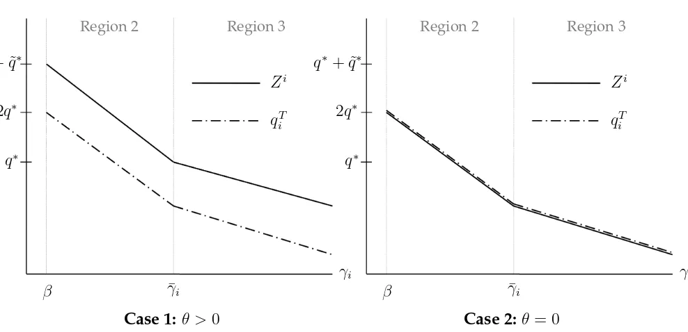
The typical buyeri’s money demand,Di
b
ε, is plotted in Figure2(for some givenbε) against the ratioϕi/(βϕbi), which captures the cost of holding home money . The money demand curve has a standard negative slope, but it also kinks at the point(m∗
i,µ¯i). Intuitively, the termµ¯i (which is shown to be greater than 1 in the appendix) captures the level of inflation that induces the buyer to carry enough money in order to purchase q∗ in the home DM.27 When the cost of
holding money drops belowµ¯i, the buyer carries an even greater amount of home currency, or, in terms of the language introduced in Lemma4, the relevant region of the FOREX bargaining protocol switches from Region 3 to Region 2. The change in the slope of the demand function around µ¯i captures the fact that the marginal benefit from carrying one more unit of money differs between Regions 2 and 3. In both Regions 2 and 3, an additional unit ofmoneyi allows buyer i to purchase more special good in DM−i if she trades in the FOREX market, a benefit which is represented by the second and third lines in equations (16), (17). However, in Region 3, an additional unit of moneyi also allows the buyer to purchase more special good in DMi, if she does not trade in the FOREX market. This benefit is represented by the fourth line in eq.(17), and it does not have a counterpart in eq.(16), since in Region 2 the buyer is already able to purchase the first-best quantity.
4
Equilibrium in the Two-Country Model
4.1
Definition of Equilibrium
In this section we characterize the steady state equilibrium of the model. Before stating the formal definition, we introduce some additional notation. LetAd
mi andA i
mi denote the amount of moneyi held by all dealers and all buyers i, respectively, at the beginning of the current period. Also, letAed
mi and Ae i
mi denote the amount of moneyi held by all dealers and all buyers
i, respectively, at the end of the preceding period. Finally, let A¯d
mi, A¯imi, and A¯−mii denote the 27In the standard one-country model, µ¯
i would be equal to 1, i.e., the buyer would carry enough money to
purchase q∗ only if the cost of holding money is zero. However, here the buyer realizes that she might have