Munich Personal RePEc Archive
Does bad company corrupts good
character? A spatial econometric analysis
of oil resource management in Africa
Ackah, Ishmael
Africa Centre for Energy Policy, Accra, Institute of Oil and Gas
Studies, University of Cape Coast
12 October 2016
1
Does bad company corrupts good character? A spatial econometric analysis of oil resource
management in Africa
Ishmael Ackah
Africa Centre for Energy Policy
Accra- Ghana and Institute of Oil and Gas Studies, University of Cape Coast
2
Abstract
A widely held belief before the 1990s – referred to as the oil-blessing hypothesis – was that oil discovery
and production should promote economic growth and development, and lead to poverty reduction.
However, the so-called ‘oil-curse’ hypothesis, postulated by Sachs and Warner in 1995, challenged this
belief, thus provoking a heated debate on the theme. The oil-curse hypothesis has been traditionally tested
by means of cross-sectional and panel-data models. We go beyond these traditional methods to test
whether the presence of spatial effects can alter the hypothesis in oil-producing African countries. In
3
the quality of democratic institutions, investment and openness to trade are investigated. Our findings
are as follows. First, the validity of the spatial Durbin model is vindicated. Second, consistently with the
oil-curse hypothesis, oil production, resources, rent and revenues have a negative and generally
significant effect on economic growth. This result is robust for across the panel data, spatial durbin, and
spatial autoregressive models, and for different measures of spatial proximity between countries. Third,
we find that the extent to which the business environment is perceived as benign for investment has a
positive and marginally effect on economic growth. Additionally, economic growth of a country is
further stimulated by a spatial proximity of a neighbouring country, if the neighbouring country has
created strong institutions protecting investments. Fourth, openness to international trade has a positive
and marginally significant effect on economic growth. However, the significance of the parameter
estimate is sensitive to the model that is being considered. Overall, the findings suggest that oil-producing
African economies are cursed by oil discovery, production and revenues rather than by the spatial
proximity with their neighboring countries.
Key words : Oil Curse, Oil Resource Governance, Africa, Spatial Analysis
1 Introduction
4
should translate into the growth of the economy by means of job creation in the oil and oil-related industries, access to credit by companies, government and individuals, technological transfer from major foreign oil companies to local partners, training and capacity building and increased government revenue through oil-related taxes and resource rent.
However, this has not been the case in most oil-producing countries, especially in Africa. Sachs and Warner (1995) propose a paradoxical hypothesis that seems to imply that oil abundance puts limits on economic growth. This hypothesis stipulates that resource-endowed countries (e.g. Nigeria, Sudan and Venezuela) are worse performers than less well-endowed countries, such as Japan, Taiwan and Korea (Sachs and Warner, 199, Tiago et al., 2010). Based on Sachs and Warner’s (1995) findings, oil resources are therefore a curse rather than a blessing. Moreover Atkinson and Hamilton (2003) posit that the inability of resource-rich countries to translate resource wealth into development may be the source of the curse. This paradoxical hypothesis suggests a shift from the classic conception of the growth-enhancing effect of rich natural resource endowments to a growth-inhibiting effect termed the oil curse.
The purpose of sustainable development is to satisfy the needs of today’s generation whilst taking into consideration the needs of future generations and the environment. To achieve this goal, Baumgartner and Quaas (2009) recommend that natural resources should be used in three ways. First, scarce and non-renewable natural resources can be used in alternative ways to achieve a number of goals. For instance, instead of exclusive reliance on oil resources, the economy should be geared towards both oil and non-oil natural resources (e.g. agriculture) to enhance sustainability. This calls for diversification of the income from natural resources. Second, scarce resources can be used to achieve alternative goals. For instance, natural resource revenues can be invested in power production and distribution to enhance electricity access which can help minimise rural poverty and rural-urban migration. Finally, scarce resources can be used to achieve some other legitimate societal goals such as establishing social or economic mitigation funds.
5
high degree of homogeneity across the countries under study. Koedijk et al. (2011) suggest that homogeneous estimates can exhibit large biases that may provoke wrong inferences and recommend heterogeneous estimation.
Since the 1960s, African countries have mooted the idea of an economic union just like that of the European Union. As a result, international institutions such as the Economic Community of West African States (ECOWAS), the African Union (AU) and the New Partnership for Africa’s Development (NEPAD) have been formed. In addition to the existing trade and cultural relations among African countries, there is an assumption that major developments and policies in one country can affect other countries. This assumption is empirically validated by Ellison and Glaesar (1997) who find that agglomeration or spatial concentration lead to regional socio-economic and technological spill overs.
These effects arising from the spatial agglomeration of countries have not properly been accounted for in previous studies. According to Damette and Seghir (2013), existing studies that have estimated the oil curse feature two main weaknesses. First, these models assume the same effect of natural resources on economic growth in all countries. As countries have different quantities of reserves, production capacity and reliance on oil revenues, this assumption may lead to unreliable estimates. Second, the constant effect of natural resources is another widely held assumption in existing studies. In practice, due to oil price and production volatility, the amounts of oil revenues differ from period to period. Third, regional studies, especially those that are based on neoclassical thought, assume that the economy is closed (Solow, 1956). However, the use of regional data opens up the possibility that the variables are not independent due to the interconnectedness of contiguous countries (Anselin, 1988). If such interconnections are not factored into the modelling, bias and inefficient estimates may arise (Buccellato, 2007). Indeed, there is evidence of cross-border contagion (Easterly and Levines, 1998).
6
econometric model; ii) the use of diagnostic tests to examine the presence of spatial dependence or heterogeneity; iii) the ability to interpolate or predict spatial effects. The contribution of this study is threefold. First, the study estimates whether there is spatial dependence between the observations by taking into consideration the location of the data measured in space. The second contribution is to ascertain whether there is spatial heterogeneity among the variables and how this affects the oil revenue– economic growth nexus. Finally, cross-country heterogeneity and the time variability of the relationship between oil revenues and economic growth determinants are also major components of the model.
2. Literature Review
Several methodologies have been developed to test the oil and natural resource curse hypothesis. For instance, Matsuyama (1992) applies the linkage approach to study the natural resource curse. He concludes that factors that push the labour force from the manufacturing sector to the primary sector slow economic growth. This is because the learning-induced positive effects in manufacturing that enhance productivity are reduced. In contrast, Sachs and Warner (1999) argue that such an approach is applicable to primary sectors such as agriculture and not the oil sector. As a remedy for the apparent deficiencies of
Matsuyama’s (1992) approach, Sachs and Warner (1995) decompose the linkage into the tradable natural
resource sector, the tradable non-natural resource sector and the non-tradable sector. They find that the greater the natural resource endowment, the greater the demand for non-tradable goods and the lesser the capital and labour allocation to the manufacturing sector. This implies that oil endowment slows industrial growth.
Extending the oil curse debate, Collier (2008) argues that the oil curse can be explained by factors other than resource abundancies, such as institutional quality, lack of skilled managers and labourers for resource governance, geographic location and other regional factors. These make the analyses of spatial effects within the relationship between oil revenues and economic growth relevant in reaching a valid conclusion. Table 1 shows a summary of studies on the relationship between oil revenues and economic growth.
Table 1. Summary of works on the oil curse hypothesis
7
Sachs and Warner (1995)
OLS 1970–
1989
Economies with high amounts of natural resources tend to have slow growth
Atkinson and
Hamilton (2003)
OLS 1980–
1995
Confirms the oil curse hypothesis
Kronenberg (2004) Stepwise regression 1989–
1999
Confirms the oil curse hypothesis
Brunnschweiler (2008)
Two-stage least
squares
1970– 2000
Oil abundance promotes economic growth
Alexeev and Conrad (2009)
Abundance of oil and other natural resources have a positive impact on economic growth
Mehrara (2009) Panel fixed effects 1965–
2005
Growth rate of oil revenues beyond the 18% threshold has a negative impact on economic growth
Cavalcanti et al
(2011)
Panel analysis 1980–
2006
Oil abundance affects growth positively
Fan et al (2012) Functional
co-efficient model
1997– 2005
Resource abundance has a positive effect on cities
Cotet and Tsui
(2013)
Dynamic panel
models
1970– 2000
Stable and positive relationship between oil abundance and long-term economic growth
Yaduma et al (2013) GMM 1980–
2007
Evidence of oil curse in non-OECD countries
A cursory look at the literature on the oil resource-economic growth nexus indicates a lack of consensus on the oil curse hypothesis. First, the findings in the literature are far from conclusive. Whilst a strand of the literature shows that oil resources have a positive effect on growth, other research provides evidence to the contrary. This necessitates the application of a new and rigorous methodology. Second, although Sachs and Warner (1997) suggest that geographical influence may be able partially to explain the oil
8
dynamics on the oil curse hypothesis. However, Fan et al. (2012) study centres on China and examines how the distance between cities influences natural resource management. Unlike Fan et al. (2012), this study examines the cross-country effect and the impact of economic distance on how oil resources have contributed to growth in Africa. Agnew and Corbridge (1989) indicate that the concept of spatiality can be taken to imply the effect of geographical entities such as distance, districts, regions and structural and economic concepts (e.g. trade) on economic growth. Furthermore, Herbert- Burns (2012) posits that the concept of space (spatial attributes) is relevant to the study of oil resource management.
In a nutshell, for the purpose of effective testing, measurability and to contribute to literature, 4 hypothesis are proposed:
i. Benign business environment of oil producing countries have spatial spill over effects on neighbouring oil producing countries.
ii. Oil revenues, oil production and oil revenues have positive effect on economic growth in oil producing African countries
iii. The method applied (cross-sectional, panel or spatial panel method) does not alter the findings on relationship between oil resources and economic growth
iv. Quality institutions have significant relationship with economic growth in oil producing African countries
3. Methods
3.1. Data
This study uses a standard cross-sectional approach, with panel data and spatial econometrics to study the oil resource–economic growth nexus. The time dimension consists of annual data spanning a period of 26 years, from 1985 to 2011. The cross-section of countries is dictated by the International Energy Agency (IEA) in terms of countries that have been producing oil over the sample period. These include
9
only countries for which oil production data have consistently been recorded from 1985 are considered. Out of these countries, Nigeria, Algeria, Angola and Libya are the major producers. According to the
EIA (2013), Africa’s oil reserves have grown by 120% in the last 30 years, from 57 billion in 1980 to
USD 124 billion barrels in 2012. In 2010, Africa contributed 12.4% of global crude oil production (KPMG, 2013).
Africa’s growth has been punctuated by social and economic tensions, conflicts, corruption and
global economic events (AEO, 2013). Despite these challenges, Africa recorded a growth rate of 6.6% in 2012, dropping to 4.8% in 2013 and projected to be 5.3% in 2014. This growth has principally been driven by high prices of commodities such as oil. Similar to the studies of Sachs and Warner (1995) and Yaduma et al (2013), this research uses vital determinants of economic growth, including trade openness, oil revenues and investment, as well as governance indicators, such as corruption and institutional quality. Institutional quality is proxied by the polity index. It is assumed that the oil curse is more pronounced in countries with poor institutional frameworks than in countries with quality institutions (Boschini et al. 2007). Indeed, investment in productive sectors and rent-seeking activities compete for oil revenues in countries with poor institutions. According to Mehlum et al. (2006), the prudent management of oil revenues in Norway and the US can be attributed to well-defined property rights and good quality and transparent institutions. On the other hand, dysfunctional institutions which promote rent-seeking behaviour have been cited as a key cause of poor management of oil revenues in Nigeria and Venezuela (Lane and Tornell, 1999).
Following the work of Yaduma et al. (2013), the sum of exports and imports as a percentage of GDP is used to measure trade openness. Yaduma et al. (2013) argue that trade opens an economy to the outside world and serves as a channel for technological transfer, which boosts economic growth. Other variables that are considered in the study include investment, computed as domestic investment as a percentage of GDP. Again, energy consumption, which has been found to be a major driver of industrialization (Stern, 2003) is included as a predictor of growth. Due to lack of complete data, Libya and Equatorial Guinea are excluded from this study.
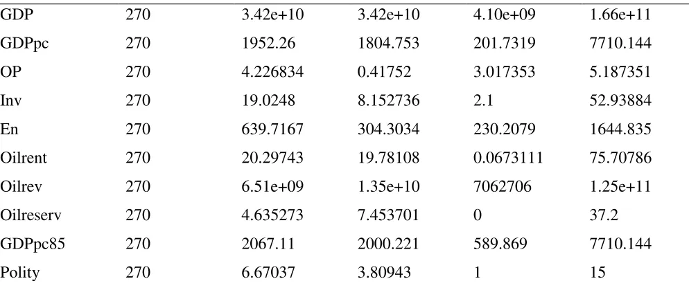
Table 2. Descriptive Statistics
10
GDP 270 3.42e+10 3.42e+10 4.10e+09 1.66e+11
GDPpc 270 1952.26 1804.753 201.7319 7710.144
OP 270 4.226834 0.41752 3.017353 5.187351
Inv 270 19.0248 8.152736 2.1 52.93884
En 270 639.7167 304.3034 230.2079 1644.835
Oilrent 270 20.29743 19.78108 0.0673111 75.70786
Oilrev 270 6.51e+09 1.35e+10 7062706 1.25e+11
Oilreserv 270 4.635273 7.453701 0 37.2
GDPpc85 270 2067.11 2000.221 589.869 7710.144
Polity 270 6.67037 3.80943 1 15
Notes: GDP is real GDP, GDPpc is real GDP per capita, OP is oil production, Inv is investment, En is energy consumption, Oilrent is oil rent, Oilrev is oil revenues, Oilreserv is oil reserves and Polity is a proxy for institutional quality. The estimation period is 1985 to 2011. The countries used in this study
are Algeria, Angola, Cameroon, Congo, the Cote d’Ivoire, Egypt, Equatorial Guinea, Gabon, Libya,
Nigeria and Sudan. GDP per capita is measured in current US dollars. Oil producing countries such as Chad, Equatorial Guinea, Libya and Sudan were exempted because there were no continuous data on some of the variables used in this study.
Time series plots of oil revenues and GDP are provided in Fig. 1. Interestingly, most African countries
seem to be diversifying since the relative share of oil revenue in GDP is low in almost all countries
[image:11.612.62.559.54.262.2]except in Angola, Gabon and Nigeria.
12
Time series plots of oil revenues and GDP in oil-producing African countries. Notes: this figure depicts
time series plots of renewable energy consumption of 9 oil-producing African countries. The sample
period runs from 1985 to 2011 for 9 countries (Algeria, Angola, Cameroon, Congo, Democratic Republic
of Congo, Côte d׳Ivoire, Egypt, Gabon, Nigeria, and Tunisia). Renewable energy consumption is
measured in current US dollars).
Four different measurements of oil abundance are used in this paper. The first is oil production in thousand barrels per day, the second is oil revenues in current US dollars, the third is oil rent in current US dollars and the final indicator is oil reserves in billion barrels. All the oil abundance indicators are obtained from the Energy Information Administration (EIA). Polity, a proxy for institutional quality, draws on Yaduma et al (2013), who also define institutional quality in a similar manner. According to Lane and Tornell (1999) and Mehlum et al. (2006), the difference between highly performing oil-producing countries, such as Norway, and under-performing oil-oil-producing countries, like Nigeria and Cameroun, can be attributed to institutional quality. Indeed institutions with poor quality enhance rent-seeking and revenue-grabbing behaviour. Polity takes on values ranging from one to ten, with the lowest values indicating countries with institutions of low quality. The data are obtained from the Polity IV project of the Centre for Systemic Peace (http://www.systemicpeace.org/polity/polity4.htm), which is similar to the data used by Wagner (2011) to measure institutional quality. Consistent with the resource abundance–growth nexus literature, other factors include energy use (measured in kilograms per oil
0 1E+10 2E+10 3E+10 4E+10 5E+10
1985 1987 1989 1991 1993 1995 1997 1999 2001 2003 2005 2007 2009 2011
Tunisia
13
equivalent per capita), trade openness (a ratio of export and imports in current US dollars) and investment (in current US dollars). Please see appendix A for the definition of the variables.
3.2. Methodology
Spatial econometric methods have gained prominence in economics for two main reasons (Anselin, 2001). The first is the desire to apply theoretical economic models that explicitly account for the interaction between an economic agent and other heterogeneous agents in a system. Indeed, these models consider factors such as neighbourhood effects, social norms, economic groupings and peer group effects and capture how individual interactions can lead to aggregate patterns. For instance, there is spatial correlation when a variable of interest (per capita growth) in location A is determined by the values of the same variable in location B. The second driver is the need to handle spatial data when there is spatial autocorrelation which cannot be captured by standard econometric methods. This paper investigates the presence of spatial effects by studying the spatial heterogeneity and the spatial correlation between per capita oil revenues and per capita economic growth. The study draws on the augmented Solow growth model suggested by Mankiw et al. (1992) and Easterly and Levine (1998) in a spatial panel analysis. As oil is traded on the international market, oil price shocks and other factors related to oil revenue management in one country can affect the growth of a neighbouring country. An example is given by the oil exploration issues involving Nigeria and Cameroon, where litigation concerning maritime border challenges has affected the oil output of both countries (Frynas and Mellahi, 2003). Another factor may be the effect of conflicts in one oil-producing country, such as Nigeria, on the growth of another, such as Cameroon. A case in point is the Boko Haram threat in Northern Nigeria which is affecting oil operations in Chad and Cameroon. This makes spatial panel data analysis suitable for this study as it captures the effect of shocks to per capita income growth of one country on the growth of another country.
According to Anselin (2001), the most common form of spatial econometric model is one that relates the value of a random variable in a given location (A) to its values in another location (B). This implies that a random variable is indexed to location j:
14
where D is a set of discrete locations or a continuous surface. As each random variable is assumed to be influenced by location, the spatial correlation can then be specified as:
covy yj, iE y y j, iE y j .E yi (2)
where ji; j and i are the individual locations; y yj, i are the values of a random variable at locations j
and i. Anselin (2001) suggests that the covariance can be estimated in three fundamental ways. First, a functional form can be estimated based on equation (1) so that the covariance structure can follow. Second, the covariance structure can be estimated directly as a function of selected parameters. Finally, the spatial equation can be modelled non-parametrically by leaving the covariance structure unspecified. Taking an N1 vector of random variables, y, observed across space and an N1 vector of independent and identically distributed (iid) random errors
, the spatial stochastic model is derived as follows:
yi
W y
i
(3)where is the mean of y, i is an N1 vector of ones, whilst is the spatial autoregressive parameter. W is the spatial weight matrix, which depends on the definition of neighbourhood for each observation. The spatial weight matrix can then be defined as:
1....,
.
ij j j
j N
Wy w y
(4)To estimate the determinants of economic growth in oil-producing African countries, GDP can be expressed as a function of the predictors defined in Table 2. This will allow the estimation of the cross section and the panel methods before the spatial variables are introduced.
The empirical model is specified as:
0 1 2 3 4 5
t t T t t t t t t t
15
Oil rent, oil production, oil revenues and oil reserves are entered in turn separately in the equation. In addition, is an unobservable country effect, t is an unobservable time effect that is common to all
countries and t is an unobservable component that varies over time and country and is assumed to be
uncorrelated. According to Madariaga and Poncent (2007), the introduction of a lagged dependent variable and country-specific effects in Equation (5) may render the OLS estimator biased and inconsistent.
To analyse the stability of the parameter estimates, we also estimate Equation (5) by replacing oil production with oil revenues, oil rent, oil reserves and energy use. In addition, we estimate the cross-sectional equation without an oil abundance variable. The specific indicators of institutional quality are the investment risk profile (the higher the value, the lower the perceived risk of investment) and the corruption index with a higher value indicating higher levels of corruption. Moreover, we estimate the panel data model without the measure of openness to trade. The estimation results for the panel method are summarized in Tables 4 (𝑶𝒊,𝒕 = oil production), 5 (𝑶𝒊,𝒕 = oil revenues), 6 (𝑶𝒊,𝒕 = oil rent) and 7 (𝑶𝒊,𝒕 = oil reserves).
However, ignoring the spatial effects could also lead to misspecification and invalid inference. The spatial effects equation can be expressed as:
yWyX (6)
where y is a vector of observations for the dependent variable, is a spatial autoregressive that takes
16
0 1 2 3 4 5 6 7
t t T t t t t t t t t t
gdp gdp oilrent inv en open polity wgdp woilrent (7)
4. Estimation Results
In Section 4.1, the estimation results from a standard cross-sectional model that draws on Sachs and Warner (1995) are analysed. In Section 4.2, the results of a standard panel-data model with cross-sectional and time fixed effects are estimated and discussed. Section 4.3 summarizes and analyses the results of the spatial Durbin model (SDM) and the spatial autoregressive model (SAR).
4.1. Cross-sectional estimation
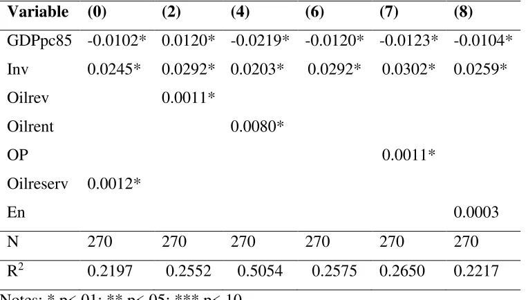
[image:17.612.57.439.337.554.2]Using a cross-sectional estimation method à la Sachs and Warner (1995), we test the growth effects of oil abundance. The results is presented in table 3
Table 7.3. Cross-sectional estimation, real GDPpc growth as the dependent variable
Variable (0) (2) (4) (6) (7) (8)
GDPpc85 -0.0102* 0.0120* -0.0219* -0.0120* -0.0123* -0.0104*
Inv 0.0245* 0.0292* 0.0203* 0.0292* 0.0302* 0.0259*
Oilrev 0.0011*
Oilrent 0.0080*
OP 0.0011*
Oilreserv 0.0012*
En 0.0003
N 270 270 270 270 270 270
R2 0.2197 0.2552 0.5054 0.2575 0.2650 0.2217
Notes: * p<.01; ** p<.05; *** p<.10
17
the Cote d’Ivoire, Egypt, Equatorial Guinea, Gabon, Libya, Nigeria and Sudan. Table 3 indicates that the
logarithm of initial real GDP per capita has the expected negative and significant effect on the average growth rate of real GDP per capita. The effect size is also stable across the six equations, except for the equation that features oil rent. Therefore, consistent with classic growth theory, poorer countries show a tendency initially to catch up with richer countries.
The average investment share in GDP has the expected positive and significant effect on the average growth rate of real GDP per capita. The effect magnitude is stable across the six equations. Therefore, higher proportional investment as a share of GDP is associated with greater economic growth. This calls for investments especially in the productive sectors of the economy such as power generation to stimulate economic growth.
Next, the oil abundance variable has a positive and significant effect, except for the equation featuring energy use. This result initially suggests that in oil-exporting African countries the resource blessing prevails. The coefficient of determination 𝑹𝟐 ranges from 22% (the equation without an oil abundance variable) to 51% (the equation featuring oil rent as an oil abundance variable).
This notwithstanding, the disadvantages of the cross-sectional method has been highlighted by a number of studies. According to Cavalcanti et al. (2011), the cross-sectional regression methodology does not take into consideration the time dimension of the data and, consequently, may suffer from endogeneity bias. Further, there is difficulty in making causal inference and the results may be different if another time-frame is used (Bland, 2001). Based on these limitations, a robust method that takes into consideration the time and geographic dimensions is used in this study.
4.2. Panel data estimation
18
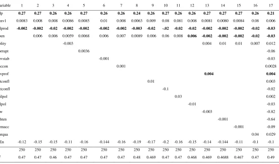
Table 4. Panel estimation with country-specific and time-specific fixed effects
Variable 1 2 3 4 5 6 7 8 9 10 11 12 13 14 15 16 17
gdp 0.27 0.27 0.26 0.26 0.27 0.26 0.26 0.24 0.26 0.27 0.26 0.26 0.27 0.27 0.27 0.26 0.21
lrinv1 0.0083 0.008 0.008 0.0086 0.0085 0.01 0.008 0.0063 0.009 0.08 0.081 0.008 0.0081 0.0080 0.0084 0.08 0.006
oilprod -0.002 -0.002 -0.02 -0.002 -0.002 -0.002 -0.002 -0.003 -0.02 -.02 -0.02 -0.02 -0.002 -0.002 -0.002 -0.02 -0.03
open 0.006 0.006 0.0059 0.0068 0.006 0.007 0.0089 0.006 0.06 0.008 0.006 -0.002 -0.002 -0.002 -0.02 -0.03
polity -0.003 0.004 0.01 0.01 0.007 0.012
corrupt 0.0036 -0.06
govstab -0.001 -0.03
soccon 0.001 0.0028
invprof 0.004 0.004
intconfl 0.01 0.003
extconfl -0.1 -0.02
milpol 0.03 0.002
relpol -0.01 -0.03
law -0.003 -0.82
ethten -0.001 -0.64
demacc -0.001 -0.09
burqua 0.04 0.029
En -0.12 -0.15 -0.15 -0.11 -0.16 -0.144 -0.16 -0.19 -0.17 -0.2 -0.16 -0.15 -0.14 -0.144 -0.11 -0.1 -0.1
N 250 250 250 250 250 250 250 250 250 250 250 250 250 250 250 250 250
R2 0.47 0.47 0.46 0.47 0.47 0.47 0.47 0.48 0.469 0.47 0.47 0.468 0.469 0.4688 0.467 0.47 0.49
19
20
Tables 4 to 7 present the results of the panel estimations. The choice of panel fixed-effects methods was informed by the results of the Hausman tests. However, Clark and Linzer (2012) argue that the Hausman test is not a sufficient metric for deciding between fixed- and random-effects models. The best metrics are the size of the dataset, the level of correlation between the covariate and unit effects and the extent of within-unit variation between the dependent and the explanatory variables (Clark and Linzer, 2012). In a large dataset with a high number of observations, the fixed-effects model produces unbiased estimates (Gelman and Hill, 2007). Therefore, this paper draws on the Hausman test and the high number of observations to establish the use of the fixed-effects model.
Four different equations are estimated with oil production, oil reserves, oil revenues and oil rents respectively. The results shown in Table 4 indicate that oil production has an inverse relationship with economic growth in all the equations estimated. Although previous studies, such as Barnett and Ossowski (2002), have used oil revenues as a proxy for oil abundance, this finding has potential policy implications. Oil production has both positive and negative effects on economic growth. First, the beginning of commercial production can offer the oil-producing country the opportunity to access the financial market as the country becomes attractive for foreign direct investments (Ross, 2012). However, oil production also has disadvantages. First, Matsuyama (2002) finds that oil production attracts labour from the other sectors of the economy and reduces productivity in these sectors. For instance, universities start introducing petroleum-related courses and radio and television discussions begin to centre on crude oil production. This affects the growth of non-oil sectors, which reduces the overall economic performance of the country. Second, oil production becomes the central focus of every major economic policy to the disadvantage of the other sectors of the economy. For example, the contribution of the agricultural sector
to Ghana’s GDP before oil production was 31% in 2008. After three years of oil production, the
21
22
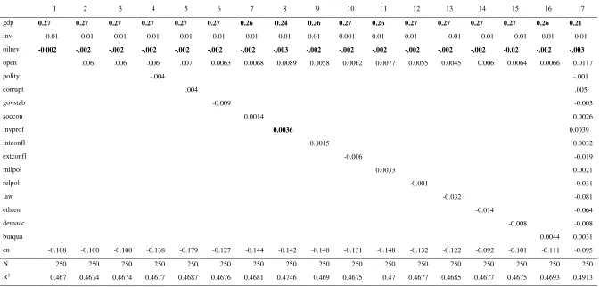
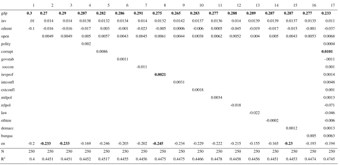
Table 5. Panel estimation with country-specific and time-specific fixed effects
1 2 3 4 5 6 7 8 9 10 11 12 13 14 15 16 17
gdp 0.27 0.27 0.27 0.27 0.27 0.27 0.26 0.24 0.26 0.27 0.26 0.27 0.27 0.27 0.27 0.26 0.21
inv 0.01 0.01 0.01 0.01 0.01 0.01 0.01 0.01 0.01 0.001 0.01 0.01 0.01 0.01 0.01 0.01 0.01
oilrev -0.002 -.002 -.002 -.002 -.002 -.002 -.002 -.003 -.002 -.002 -.002 -.002 -.002 -.002 -0.02 -.002 -.003
open .006 .006 .006 .007 0.0063 0.0068 0.0089 0.0058 0.0062 0.0077 0.0055 0.0045 0.006 0.0064 0.0066 0.0117
polity -.004 -.001
corrupt .004 .005
govstab -0.009 -0.003
soccon 0.0014 0.0026
invprof 0.0036 0.0039
intconfl 0.0015 0.0032
extconfl -0.006 -0.019
milpol 0.0033 0.0021
relpol -0.001 -0.031
law -0.032 -0.081
ethten -0.014 -0.064
demacc -0.008 -0.008
burqua 0.0044 0.0031
en -0.108 -0.100 -0.100 -0.138 -0.179 -0.127 -0.144 -0.142 -0.148 -0.131 -0.148 -0.132 -0.122 -0.092 -0.101 -0.111 -0.095
N 250 250 250 250 250 250 250 250 250 250 250 250 250 250 250 250 250
R2 0.467 0.4674 0.4674 0.4677 0.4687 0.4676 0.4681 0.4746 0.469 0.4675 0.47 0.4677 0.4685 0.4677 0.4675 0.4693 0.4913
23
24
Table 5 shows the results for the determinants of economic growth in oil-producing African countries. In this section, the results for the impact of oil revenues, governance variables and energy consumption on economic growth are presented. Consistent with the findings of Sachs and Warner (1995), Gyfalson (2001), Atkinson and Hamilton (2003) and Yaduma et al. (2013), there is an inverse relationship between economic growth and oil revenues in oil-producing African countries. Lane and Tornell (1996) attribute this to excessive rent-seeking behaviour, corruption and weak
institutions, which they term ‘voracity effects’. This notwithstanding, two circumstances can explain this finding. First, as oil revenues are seen as ‘given by nature’, citizens’ demand for accountability
25
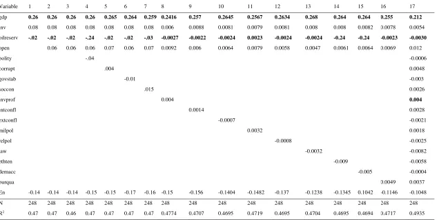
Table 6. Panel estimation with country-specific and time-specific fixed effects
1 2 3 4 5 6 7 8 9 10 11 12 13 14 15 16 17
gdp 0.3 0.27 0.29 0.287 0.282 0.286 0.291 0.275 0.265 0.283 0.277 0.288 0.289 0.287 0.287 0.277 0.233
inv .01 0.014 0.014 0.0138 0.0132 0.0134 0.014 0.0132 0.0142 0.0137 0.0136 0.014 0.0139 0.0139 0.0137 0.0135 0.011
oilrent -0.1 -0.016 -0.016 -0.017 0.003 -0.001 -0.023 -0.005 0.0006 -0.006 0.0005 -0.045 -0.019 -0.017 -0.015 -0.001 -0.037
open 0.0049 0.0049 0.005 0.0057 0.0043 0.0045 0.0061 0.0044 0.0038 0.0062 0.0052 0.004 0.005 0.0043 0.0053 0.0068
polity 0.002 0.0004
corrupt 0.0086 0.0101
govstab 0.0011 -.0011
soccon -0.011 0.001
invprof 0.0021 0.0014
intconfl 0.0031 0.0048
extconfl 0.0018 0.001
milpol 0.0034 0.0013
relpol -0.018 -0.071
law -0.022 -0.046
ethten -0.0002 -0.006
demacc 0.0012 0.0013
burqua 0.005 0.0063
en -0.2 -0.233 -0.233 -0.169 -0.246 -0.203 -0.202 -0.245 -0.234 -0.229 -0.222 -0.215 -0.155 -0.165 -0.23 -0.193 -0.194
N 250 250 250 250 250 250 250 250 250 250 250 250 250 250 250 250 250
R2 0.4 0.4451 0.4451 0.4452 0.4517 0.4455 0.4456 0.4475 0.4475 0.4466 0.4478 0.4458 0.4456 0.4451 0.4453 0.4474 0.4745
26
27
28
Table 7 Panel estimation with country-specific and time-specific fixed effects (real GDPpc growth as the dependent variable)
Variable 1 2 3 4 5 6 7 8 9 10 11 12 13 14 15 16 17
gdp 0.26 0.26 0.26 0.26 0.265 0.264 0.259 0.2416 0.257 0.2645 0.2567 0.2634 0.268 0.264 0.264 0.255 0.212
inv 0.08 0.08 0.08 0.08 0.08 0.08 0.08 0.006 0.0088 0.0081 0.0079 0.0081 0.008 0.008 0.0082 0.0078 0.0054
oilreserv -.02 -.02 -.02 -.24 -.02 -.02 -.03 -0.0027 -0.0022 -0.0024 0.0023 -0.0024 -0.0024 -0.24 -0.24 -0.0023 -0.0030
open 0.06 0.06 0.06 0.07 0.06 0.07 0.0092 0.006 0.0064 0.0079 0.0058 0.0047 0.0061 0.0064 0.0069 0.012
polity -.04 -0.0006
corrupt .004 0.0048
govstab -0.01 -0.003
soccon .015 0.0026
invprof 0.004 0.004
intconfl 0.0014 0.0028
extconfl -0.0007 -0.0021
milpol 0.0032 0.0018
relpol -0.0008 -0.0025
law -0.0032 -0.0082
ethten -0.009 -0.0058
demacc -0.005 -0.0004
burqua 0.0049 0.0037
En -0.14 -0.14 -0.14 -0.15 -0.15 -0.17 -0.16 -0.15 -0.156 -0.1404 -0.1482 -0.137 -0.1238 -0.1345 0.1042 -0.1146 -0.1048
N 248 248 248 248 248 248 248 248 248 248 248 248 248 248 248 248 248
29
30
Finally, Table 7 presents the results of the ‘oil reserve’ equation. According to Stijns (2005), natural resource reserves have had an inverse relationship with economic growth since the 1970s. As reserves represent a future revenue stream, policy makers may be tempted to spend more today and pay with the production of the reserves tomorrow. Another explanation for the inverse relationship between economic growth and reserves is ‘feeding frenzy’. Lane and Tornell (1996) argue that the discovery of natural resources leads to a fight for control and spending between competing factions, which leads to inefficiency, this being termed a ‘feeding
frenzy’. Without any long-term planning or accountability in institutions, such spending can lead to waste and corruption, thereby affecting growth negatively. Table 8 reveals this trend
and supports Stijns’ (2005) assertion that reserves generally have a negative impact on growth. Furthermore, and consistent with other findings, the investment profile of the countries has a positive impact on economic growth.
4.3 Spatial model
31
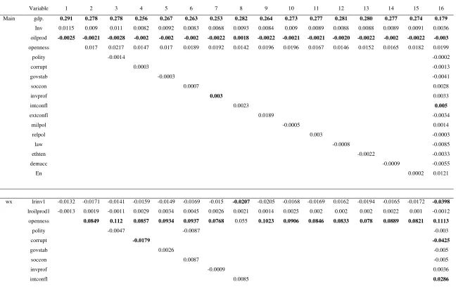
Table 8. Spatial Durbin model (SDM)
Variable 1 2 3 4 5 6 7 8 9 10 11 12 13 14 15 16
Main gdp. 0.291 0.278 0.278 0.256 0.267 0.263 0.253 0.282 0.264 0.273 0.277 0.281 0.280 0.277 0.274 0.179
Inv 0.0115 0.009 0.011 0.0082 0.0092 0.0083 0.0068 0.0093 0.0084 0.009 0.0089 0.0088 0.0088 0.0089 0.0091 0.0036
oilprod -0.0025 -0.0021 -0.0028 -0.002 -0.002 -0.002 -0.0022 0.0018 -0.0022 -0.0021 -0.0021 -0.0020 -0.0022 -0.002 -0.0022 -0.003
openness 0.017 0.0217 0.0147 0.017 0.0189 0.0192 0.0142 0.0196 0.0196 0.0167 0.0146 0.0152 0.0165 0.0182 0.0199
polity -0.0014 -0.0002
corrupt 0.0003 -0.0013
govstab -0.0003 -0.0041
soccon 0.0007 0.0028
invprof 0.003 0.0033
intconfl 0.0023 0.005
extconfl 0.0189 -0.0034
milpol -0.0005 0.0014
relpol 0.003 -0.0003
law -0.0008 -0.0085
ethten -0.0022 -0.0033
demacc -0.0009 -0.0055
En 0.0002 0.0121
wx lrinv1 -0.0132 -0.0171 -0.0141 -0.0159 -0.0149 -0.0169 -0.015 -0.0207 -0.0205 -0.0168 -0.0169 0.0162 -0.0194 -0.0165 -0.0172 -0.0398
lroilprod1 -0.0013 0.0019 -0.0011 0.0029 0.0034 0.0045 0.0026 0.0021 0.0014 0.0025 0.002 0.002 0.002 0.0022 0.001 -0.0012
openness 0.0849 0.112 0.0857 0.0934 0.0937 0.0768 0.055 0.1023 0.0906 0.0846 0.0833 0.078 0.0889 0.0821 0.1113
polity -0.0047 -0.0087 -0.003
corrupt -0.0179 -0.0425
govstab 0.0026 -0.005
soccon 0.0087 -0.005
invprof -0.0009 0.0036
32
extconfl -0.0044 -0.013
milpol -0.0036 -0.0084
relpol 0.0153
law 0.0045 -0.0254
ethten 0.0147 0.0418
demacc -0.0018 -0.043
En 0.0034 0.0402
rho 0.1974 0.112 0.0355 0.0593 0.0782 0.1133 0.1236 0.081 0.0844 0.1108 0.1127 0.1076 0.0884 0.1103 0.1138 0.2418 Variance 0.0019 0.0018 0.0018 0.0018 0.0018 0.0018 0.0018 0.0018 0.0018 0.0018 0.0018 0.0018 0.0018 0.0018 0.0018 0.0016 Direct. Inv 0.0117 0.0093 0.0116 0.0087 0.0096 0.0087 0.0072 0.0097 0.0088 0.0094 0.0093 0.0092 0.0092 0.0093 0.0095 0.0055
oilprod -0.0025 -0.0020 -0.0028 -0.0015 -0.0018 -0.0019 -0.0021 -0.0018 -0.0021 -0.0020 -0.0020 -0.0019 -0.0021 -0.0019 -0.0021 -0.0033
openness 0.0187 0.0222 0.0156 0.018 0.0206 0.0205 0.0149 0.0201 0.0212 0.0182 0.0159 0.0162 0.018 0.0197 0.0166
polity -0.0012 0.0001
corrupt 0.0012 0.0008
govstab 0.0002 -0.004
soccon 0.001 0.0029
invprof 0.0036 0.0029
intconfl 0.0028 0.0041
extconfl -0.0027
milpol 0.0035 0.0012
relpol -0.0002 -0.001
law -0.0011 -0.0089
ethten 0.0001 -0.0035
demacc 0.0009 -0.0047
burqua 0.0046 0.011
Indirect. Inv -0.0139 -0.0162 -0.0127 -0.0146 -0.0133 -0.0158 -0.0138 -0.0197 -0.0193 -0.0155 -0.0158 -0.0144 -0.0186 -0.0155 -0.0161 -0.0354
oilprod -0.0021 0.0025 -0.0011 0.003 0.0036 0.0048 0.0027 0.0021 0.0014 0.0028 0.002 0.0022 0.0019 0.0023 0.0009 0.0005
openness 0.1009 0.1118 0.0877 0.0976 0.105 0.0847 0.0554 0.1078 0.1027 0.0935 0.0892 0.0821 0.0989 0.0913 0.0901
33
corrupt -0.0200 -0.0348
govstab 0.0023 -0.0029
soccon -0.0102 -0.0058
invprof -0.0009 0.0018
intconfl 0.009 0.0234
extconfl -0.0049 -0.0102
milpol -0.0057 -0.0091
relpol -0.0004 0.0116
law 0.0052 -0.0212
ethten 0.0147 0.0377
demacc -0.0032 -0.0343
burqua 0.0031 0.0289
Total lrinv1 0.002 -0.0069 -0.0011 -0.0059 -0.0037 -0.0071 -0.0067 -0.0099 -0.0105 -0.0061 -0.0066 -0.0052 -0.0094 -0.0062 -0.0066 -0.029
oilprod -0.0046 0.0005 -0.0038 0.0015 0.0017 0.003 0.0006 0.0004 -0.0007 0.0008 0.0004 0.0003 -0.0002 0.0004 -0.0013 -0.0028
openness 0.1195 0.1341 0.1033 0.1156 0.1255 0.105 0.0702 0.1280 0.124 0.112 0.1051 0.0984 0.1169 0.111 0.107
polity -0.0062 -0.0018
corrupt -0.0188 -0.0340
govstab 0.0025 -0.0069
soccon -0.0093 -0.0029
invprof 0.0027 0.0048
intconfl -0.0119 0.0275
extconfl -0.005 -0.0129
milpol -0.0022 -0.0079
relpol -0.0006 0.0106
law 0.0041 -0.0301
ethten 0.0148 0.0342
demacc -0.0023 -0.039
burqua 0.0077 0.04
34
R2 0.2735 0.3181 0.3114 0.3255 0.319 0.3036 0.3179 0.3216 0.3177 0.3045 0.3191 0.3208 0.3141 0.3182 0.316 0.2979
35
An attempt is made to examine the spatial dynamics between oil resources (production, reserves, rent and revenues) and economic growth in oil-producing African countries. The
results indicate that the parameter ‘rho’ is statistically significant in all equations of the spatial
Durbin model (SDM) and the spatial autoregressive (SAR) model. This indicates that if a country grows, it positively affects the growth of its neighbours. Therefore, the spatial autoregressive effect is positive and significant. This finding is relevant to regional bodies such as the African Union and ECOWAS in initiating regional policies that improve economic growth in both regional and individual countries. Regarding the geographical effects on the relationship between oil resources and economic growth, the study finds no evidence that the proximity of countries has an impact on oil revenue management. This finding implies that
‘bad company’ does not necessarily corrupt good character but rather the actions and inactions of individual oil-producing countries affect the economic growth–oil resource management nexus. This finding therefore confirms the assertion by Sachs and Warner (2001) that geographical influence on the resource curse hypothesis may be insignificant..
Furthermore, the spatial effect of trade openness is positive but is significant only in some equations. The effect is not robust across different measures of oil variables and different models. Thus, there is some evidence that if a country is open to international trade, its neighbouring countries are likely to grow faster, but it is rather weak. Yanikkaya (2003) finds that developing economies should benefit from trade among themselves, especially when the trade encourages technical transfer. However, he argues that the impact of trade openness on economic growth is not straightforward and that trade barriers have relatively higher impact on economic growth when the country has a comparative advantage.
Consistent with the oil curse literature, corruption is found to be detrimental to economic growth in some of the models. This is because corruption diverts revenues into personal accounts that would otherwise have been used for development. Mo (2001) argues that one of the main channels in which corruption affects economic growth negatively is political instability.
36
5. Conclusion and Recommendations
The effect of oil revenues and oil abundance on economic growth in oil-producing African countries is examined in this paper by considering the spatial dynamics of this relationship. In particular, the effects on economic growth of oil production, oil resources and oil revenues, together with the quality of democratic institutions, investment and openness to trade, are investigated. The findings are as follows. First, the validity of the spatial Durbin model is vindicated. Second, consistent with the oil curse hypothesis, oil production, resources, rent and revenues have a negative and generally significant effect on economic growth. This result is robust across the panel data, spatial Durbin and spatial autoregressive models and for different measures of spatial proximity between countries. Third, the extent to which the business environment is perceived as benign for investment has a positive, albeit marginal, effect on economic growth. In addition, the economic growth of a country is further stimulated by spatial proximity to a neighbouring country if the neighbouring country has created strong institutions protecting investments. Fourth, openness to international trade has a positive and marginally significant effect on economic growth. However, the significance of the parameter estimate is sensitive to the model that is being considered.
Overall, the findings suggest that oil-producing African economies are cursed by oil discovery, production and revenues, rather than by the spatial proximity to their neighbouring countries. These findings have four main policy implications. First, oil-producing African countries should do more to translate oil production and oil revenues into sustainable economic development. This can be done by adapting any of three practical models. The first is the Norwegian model. Norway invested in domestic infrastructure and human capital development in the initial stages of its oil production. Later, it created a Sovereign Wealth Fund and now
spends only the interest accruing to the fund. The second model is Indonesia’s agricultural
modernization. Indonesia invested much of its oil revenues in modernizing agriculture to boost food production, reduce food imports and create jobs, especially in rural areas. Finally,
Malaysia’s diversification model ensures that oil revenues are invested in small and medium-scale enterprises and also invests in ways that help to create an enabling business environment. These models call for capital investment at the expense of spending on goods and services.
37
and spatial effect on economic growth. This can be done by enforcing the implementation of treaties such as the Abuja Declaration, which called for high investment in agriculture, and the
New Partnership for Africa’s Development, which focuses more on trade, regional integration
and human capital development.
Third, international trade has been identified as one of the main drivers of growth in this study. Oil-producing African countries should therefore engage in value-added trade with other African countries and the international community to promote job creation and economic growth.
Fourth, with investment profile as a leading driver of economic growth, countries should create an enabling business environment by minimizing the process of establishing businesses, enforcing contracts and publishing beneficial ownership information, encouraging transparency and accountability in awarding oil production contracts and managing oil revenues.
Finally, the non-oil sector should be given considerable attention. This has three advantages: (i) the non-oil sector will become the anchor of the economy when oil productions peak and start diminishing; (ii) it will minimize the impact of oil price fluctuations on the economy and help build stability to stem volatility; (iii) as the opportunity of creating more jobs in the oil sector is minimal due to the capital-intensive nature of the sector, investing in the non-oil sector can take up labour to reduce unemployment.
References
Ackah, I. (2016). Sacrificing Cereals for Crude: Has oil discovery slowed agriculture growth in Ghana?. MPRA
Ackah, I., Kankam, D., & Appiah-Adu, K. 2014, Does a windfall lead to a downfall? A study of mineral rents and genuine growth in selected African countries.Journal of Energy and Natural Resources, 3, 6-10.
Alexeev, M., Conrad, R., 2009, The elusive curse of oil. Review of Economics and Statistics, 91(3), 586-598.
Anselin, L., 2003, Spatial externalities, spatial multipliers, and spatial econometrics.
International regional science review, 26(2), 153-166.
38
Auty, R., 2001, The political economy of resource-driven growth. European Economic Review. Atkinson, G., Hamilton, K., 2003, Savings, growth and the resource curse hypothesis. World Development, 31(11), 1793-1807.
Auty, R.M., Mikesell, R.F., 1998, Sustainable development in mineral economies. Oxford University Press.
Baumgärtner, S., & Quaas, M. F. (2009). Ecological-economic viability as a criterion of strong sustainability under uncertainty. Ecological Economics, 68(7), 2008-2020.
Brunnschweiler, C. N. (2008). Cursing the blessings? Natural resource abundance, institutions, and economic growth. World development, 36(3), 399-419.
Buccellato, T. (2007). Convergence across Russian regions: a spatial econometrics approach. Cavalcanti, T. V. D. V., Mohaddes, K., & Raissi, M. (2011). Growth, development and natural resources: New evidence using a heterogeneous panel analysis. The Quarterly Review of Economics and Finance, 51(4), 305-318.
Collier, P. (2008). Laws and codes for the resource curse. Yale Hum. Rts. & Dev. LJ, 11, 9. Corden, W. M., and Neary, P. J. 1982. "Booming Sector and De-industrialization in a Small Open Economy." Economic Journal 92.
Cotet, A. M., & Tsui, K. K. (2013). Oil, Growth, and Health: What Does the Cross‐Country Evidence Really Show?*. The Scandinavian Journal of Economics, 115(4), 1107-1137. Damette, O., & Seghir, M. (2013). Energy as a driver of growth in oil exporting countries?. Energy Economics, 37, 193-199.
Easterly, W., & Levine, R. (1998). Troubles with the neighbours: Africa's problem, Africa's opportunity. Journal of African Economies, 7(1), 120-142.
Frankel, J.A. and D. Romer, 1999. Does Trade Cause Growth? American Economic Review 89: 379-399.
Gylfason, T., 2001, Natural resources and economic growth: What is the connection? CESifo Working Paper 530.
Koedijk, K.G., Tims, B., Van Dijk, M.A., 2011, Why panel tests of purchasing power parity should allow for heterogeneous mean reversion. Journal of International Money and Finance, 30, 1, 246-267.
Krugman, P., 1987, The narrow moving band, the Dutch disease, and the competitive consequences of Mrs Thatcher. Journal of Development Economics 45, 1-28.
Lane, P.R., Tornell, A., 1996, Power, growth, and the voracity effect. Journal of Economic Growth 1, 213-241.
Madariaga, N., Poncet, S., 2007, FDI in Chinese cities: Spillovers and impact on growth. World Economy, 30(5), 837-862.
Mankiw, N.G., 1992, The reincarnation of Keynesian economics. European Economic Review, 36(2), 559-565.
39
Mehlum, H., Moene, K., Torvik, R., 2006, Institutions and the resource curse. Economic Journal, 116(508), 1-20.
Mehrara, M., 2009, Reconsidering the resource curse in oil-exporting countries. Energy Policy, 37(3), 1165-1169.
Moran, P. A., 1950, Notes on continuous stochastic phenomena. Biometrika, 17-23. Paelink, J.H.P., Klaasen, L.H. 1972, Spatial econometrics. Saxon House.
Ross, M., 2012, The oil curse: How petroleum wealth shapes the development of nations. Princeton University Press.
Rosser, A., 2006, The political economy of the resource curse: A literature survey (Vol. 268). Institute of Development Studies: Brighton, UK
Sachs, J.D., Warner, A.M., 2001, The Curse of Natural Resources. European Economic Review
45, 827-838.
Sachs, J.D., Warner, A.M., 1999, Natural resource intensity and economic growth. In:
Development Policies in Natural Resource Economies, eds. Jörg Mayer, Brian Chambers, and Ayisha Farooq. Edward Elgar, Cheltenham, UK, 13-38.
Sachs, J.D., Warner, A.M., 1995. Natural resource abundance and economic growth. NBER Working Paper Series 5398, December, 1-47.
Solow, R.M., 1956, A Contribution to the theory of economic growth. Quarterly Journal of Economics, 70(1), 65-94.