Block iterative lattice Boltzmann algorithm for linear oscillatory
flow in the frequency domain
Hang Kang a, Yong Shi a,* and Yuying Yan a, b
a Research Centre for Fluids and Thermal Engineering, The University of Nottingham Ningbo China, Ningbo 315100, People's Republic of China
b Research Group of Fluids and Thermal Engineering, The University of Nottingham, Nottingham NG7 2RD, United Kingdom
Abstract
A recent article (Y. Shi and John E. Sader, Phys. Rev. E 81, 036706 (2010)) developed a linear lattice Boltzmann (LB) model in the frequency domain to characterize the performance
of micro- and nanoelectromechanical systems (M/NEMS). Nonetheless, its numerical
algorithm is formulated in the conventional time-marching form with addition of a virtual
time scale. In this article, we propose a different algorithm to solve such a linear
frequency-dependent LB model using the block iteration scheme consisting of the tri-diagonal matrix
method and Jacobi line iteration. This change in the LB algorithm leads to straightforward
modelling of linear oscillatory flow in the frequency domain without mimicking a numerical
time evolution. Through simulating the one-dimensional oscillatory Couette flow and
two-dimensional flow around an oscillating circular cylinder, we examined numerical accuracy of
the block iterative LB algorithm proposed in this article. Importantly, we also explored
modifications under this block-iterative LB algorithmic framework through use of other
prevailing computational fluid dynamics (CFD) techniques. Computational efficiency of
these original and modified block iterative LB algorithms was compared with that of the
conventional time-marching LB algorithm. The numerical results in this article demonstrate
the block iterative LB algorithm is a useful alternative numerical solver exhibiting nearly 2nd order accuracy for simulating frequency-dependent linear oscillatory flow in MEMS and
NEMS. Our simulations also reveal rich extensions of this block iterative LB algorithm
through combining the LB theory with advanced CFD numerical techniques.
* Corresponding author. Tel: +86 (0)574 88180000 (Ext. 9413); fax: +86 (0)574 88180715
Keywords: Lattice Boltzmann algorithm; Linear Oscillatory flow; Block iteration; TDMA
1. Introduction
Over the last twenty-five years, there has been a tremendous surge of interests in the
lattice Boltzmann (LB) method, which spurred its rapid and productive development for
modelling a wide variety of physical processes [1-3]. In particular, the LB method achieved
great successes in simulating complex fluid transport phenomena, including, but not limited
to, multicomponent/multiphase flow [4, 5], suspension flow [6], flow in porous media [7, 8],
[9], flow coupled with heat and mass transfer [10, 11] and even turbulence [12]. From the
numerical point of view, the LB method possesses many distinguished advantages over
conventional computational fluid dynamics (CFD) approaches, such as its simple formulas,
parallel algorithmic structure and intrinsic particle-dynamics related framework [13].
Especially, the last feature enables the method employs some simple heuristic particle
dynamic like treatments to tackle tough numerical issues. One known representative is the
bounce-back for no-slip boundary conditions on solid walls [14]. Significantly, the LB
method has a direct link to the Boltzmann equation with Bhatnagar-Gross-Krook assumption
(Boltzmann BGK equation) [15, 16]. Many LB models for continuum flow in the literature
are derived from the Boltzmann-BGK equation in the limit of low Mach number by
appropriate discretization in the time, physical space and particle-velocity space [15]. This
theoretical foundation in the Boltzmann theory triggers recent intensive efforts in
investigating the LB capability for simulating flow beyond the Navier-Stokes order. Among
various developments are the effective mean free path models [17, 18], high-order LB
models [19, 20], half-space LB models [21-22], etc.
During almost the same period, we also witnessed great strides in micro-fabrication
technologies and nanoscience [23, 24]. Plenty of micro-and nanosize electromechanical
systems (M/NEMS) with different functions were designed and manufactured in elaborate
structures [24-26]. The broad applications of these M/NEMS provide direct practical
relevance of the LB models for flow beyond the Navier-Stokes order as the characteristic
length scales of some M/NEMS are comparable to the mean free path of working fluids,
leading to pronounced non-continuum effects in flow [24, 27].
On the other hand, not all flows in M/NEMS are non-continuum nonetheless. Many
liquid flows over wetting surfaces and even some gas flows in these miniature devices still
comparison to macroscale flow, however, the continuum flow in M/NEMS manifest itself
some distinct transport characteristics, e.g., the dominant viscous-force effects [28].
Especially, flow in some cases undergoes periodical oscillation driven by the resonating
components imbedded in M/NEMS [30, 31]. In the literature, Y. Shi et al. proposed a LB
model different from the classical version to describe this type of continuum flows in
M/NEMS [32]. They derived a LB model from the linearized Boltzmann BGK equation, and
formulated it depending on the frequency of oscillation, instead of the conventional time
scale. In so doing, this linearized LB model eliminates the intrinsic nonlinearity of the LB
method corresponding to advection, and is able to treat the oscillating structures in the flow
as fixed boundaries in its simulation [32]. Importantly, the model outputs
frequency-dependent numerical results. All these features make such a linearized LB model as a
favourable numerical tool for modelling oscillatory flow in M/NEMS, where nonlinear
advection is rather weak due to the very small Reynolds number and measurements in terms
of frequency are preferable for characterizing system performance.
However, we note this linearized LB model developed in the frequency domain was
ultimately solved numerically through use of the time-marching method [32], though it is
irrelevant to any time scale. In the literature, a massive majority, if not all, of LB models are
formulated depending on time, regardless of whether they originate from the lattice-gas
cellular automata [33, 34] or the Boltzmann BGK equation [15, 16]. It is thus not surprising
that the time-marching algorithm gain a prevailing position in the LB numerical
implementation. The linearized frequency-based LB model in Ref. [32] followed this
convention, which introduced a virtual time in its framework and modified its equation with
addition of a derivative of this time scale. As such, the model was again solved using the
time-marching method as an evolution process in the frequency domain. In this case, only
“steady-state” results are meaningful and used as true numerical outputs of the simulation.
Numerically, there do not exist any prerequisites to enforce a LB algorithm to be devised
by the time-marching method. This point is of particular importance for the above LB model
in the frequency domain [32] as its inherent linearity and time independence allow flexible
choices of numerical methods to constitute its algorithm. Actually, such a model turns into a
sparse banded linear system of algebraic equations after discretizing the physical space and
particle-velocity space. These resulting linear equations can be well solved either by direct or
iterative numerical methods with the unnecessary introduction of a virtual time scale in the
frequency domain at all [35, 36]. Two direct numerical methods, i.e., Cramer’s rule [37] and
necessitate formidable computational costs when solving a large linear system of
N algebraic equations for N unknowns, where N 1. In a Gaussian elimination, the number of arithmetic operations is approximately proportional to N3, and the operations in a
Cramer’s rule-based computation will dramatically increase up to the order of
N1 !
[36]. This computational inefficiency has significantly hindered applications of the direct methods,especially for multi-dimensional problems. Iterative methods is another category to attack a
large linear system of equations using a different computational strategy. These methods
make use of the matrix splitting technique to derive from the linear equations a sequence
amenable to iteration [35, 36]. Through this sequence, iterative methods compute the
unknowns at the nth step using the results from the previous levels, and repeat such a
recurrence until convergence is reached. The key for a good iterative method is to ensure that
the designed sequence is convergent or conditionally convergent, and its iteration proceeds
toward convergence at a fast rate [35, 36].
Interestingly, nowadays few CFD studies construct a numerical algorithm based on only
one type of methods. Instead, integration of a direct method with an iterative method is a
widespread treatment in the CFD simulation for two- and three-dimensional (2 and 3D)
problems. An example is the so-called block iteration, in which a direct method is used to
solve the unknowns simultaneously in one dimension while those in the other dimensions are
updated in an iterative manner [36]. In this article, we apply the thought of block iteration to
solve the linearized LB model in the frequency domain. To be specific, we construct a purely
frequency-dependent LB numerical algorithm based on a block iteration scheme consisting
of the tri-diagonal matrix algorithm (TDMA) [38] and Jacobi line iteration (JLI) [36].
The TDMA is a simplified Gaussian elimination, which is known for its high efficiency
for solving the large tridiagonal system of algebraic equations. In comparison to other
Gaussian elimination techniques, the operations in a TDMA-based computation are just in
the order of N. Another advantage of the TDMA is it has a large variety of variants for different problems. In this article, we will use one of its variants, i.e., the cyclic tri-diagonal
matrix algorithm (CTDMA), to simulate flow subject to periodic boundary conditions [36,
39]. Crucially, on top of the JLI just mentioned, this article also explores a stretch of the
block iterative LB algorithm (BLB) through use of other more efficient iterative methods. We
develop a set of modified BLB algorithms based on the Gaussian-Seidel line iteration (SLI)
[36], alternative direction iteration (ADI) [36, 40] and over relaxing (OR) [36]. An attempt of
algorithms are carefully examined in comparison to that of the original BLB (JLI) version
and the conventional time-marching LB (TLB) algorithm constructed based on a virtual time
scale [32], respectively.
The article is organized as follows: we first briefly introduce the linearized Boltzmann
BGK equation and the corresponding LB model in the frequency domain in Section 2. In
Section 3, the BLB algorithm based on the TDMA and JLI is developed. This algorithm is
then applied to simulate the oscillatory Couette flow and flow around an oscillating circular
cylinder in Section 4. Its numerical accuracy is validated by the available analytical solutions.
Section 4 also uses the oscillatory Couette flow as a test to analyze computational efficiency
of the BLB algorithms modified by the SLI, ADI, OR and non-uniform. A comparison of
these results with those obtained by the original BLB (JLI) and TLB algorithms is elaborated.
Finally, we draw our conclusions in Section 5, and relegate the mathematical details pertinent
to the modified BLB algorithms to Appendix A – D.
2. Linearized lattice Boltzmann model in the frequency domain
In this section, we use the linearized Boltzmann Bhatnagar-Gross-Krook (BGK) equation
as a kinetic model for linear oscillatory flows, and present its LB version in the frequency
domain.
2.1.Linearized Boltzmann-BGK equation
In the kinetic theory of gases, the well-known linearized Boltzmann BGK equation is [41]
1
( eq)
h h
h - h
t
c r , (1)
where t,rand c represent the time, particle position and particle velocity, respectively. is the relaxation time and h is a perturbation to the distribution function f from the global
equilibrium feq. It is defined as
1
eq
f h
f
In the right hand side of Eq. (1), heqrepresents a perturbation to the local equilibrium from
eq
f . This function can be formulated as a polynomial in terms of the fluid density
perturbation and velocity perturbation u, i.e.,
0 0 0
eq
h
R T
c u , (3)
where 0 and T0 are the fluid density and temperature at the global equilibrium, respectively.
0
R is the gas constant.
As pointed out in Ref. [32], use of the linear Boltzmann-BGK equation, Eq. (1), in the
frequency domain is much more convenient for simulating oscillatory flow in M/NEMS. We
thus apply the time-frequency transformation of ˆ
r c,
r c, ,t e
i t , where the radialfrequency and the imaginary unit i. In the frequency domain, the linear Boltzmann-BGK
equation becomes
ˆ ˆ* ˆ
eq
h h h
c
r , (4)
where hˆ and hˆeq are the frequency-based version of hˆ and hˆeq obtained through use of the
aforementioned time-frequency transformation. The complex relaxation time
*
1 i
. Importantly, after the transformation, Eq. (4) does not involve any time
scale in the frequency domain.
2.2.Linearized lattice Boltzmann model in the frequency domain
A linearized LB model can be derived from Eq. (4) by discretizing its physical space and
particle velocity space. For simplicity while without loss of generality, we only consider 2-D
flow in this article. Furthermore, we point out that the following derivation does not involve
temporal discretization. This contrasts to the conventional discretization procedure used to
Discretization starts from the particle velocity space in Eq. (4). In this article, the popular
D2Q9 discrete particle velocity space [42] is used, in which the corresponding discrete
particle velocities are
0, 0 , 0,
cos 1 2 , sin 1 2 , 1, 2, 3, 4,
2 cos 2 9 4 , sin 2 9 4 ,
j j
j
c c j j j
c j j
c e
5, 6, 7, 8.
j (5)
where c is the particle speed and ej is the unit vector in the direction of the th
j discrete
particle velocity. With this D2Q9-based discretization, Eq. (4) is reduced to
*
ˆ ˆ ˆeq
j j j
j
h h h
c e
r , (6)
where hˆj and hˆeqj are the discrete particle-velocity versions of hˆ and hˆeq. hˆeqj is further
expressed as
0 0
ˆ ˆ
ˆeq j
j c h RT
e u. (7)
In Eq. (7), ˆ and ˆu denote the fluid property perturbations in the form depending on the frequency. They are computed by [32]
0 ˆ
ˆ j j
j
w h
, ˆ jˆj jj
w h c
u e . (8)
The moment weights, wj, in the D2Q9 space are specified [42]
4 / 9, 0,
1 / 9, 1, 2, 3, 4,
1 / 36, 5, 6, 7, 8.
Next, we extend discretization to the physical space in Eq. (6) using the finite difference
schemes. In this section, two finite difference schemes are assigned to approximate the
spatial gradient on the left hand of Eq. (6). For better demonstration, we take a spatial
gradient with respect to x in Cartesian coordinates as an example. We approximate this
gradient on a bulk node,
xm,yn
, using the second-order upwind finite difference scheme (SUS) [36], i.e.,
2
( , )
ˆ ˆ ˆ
ˆ 3 , 4 , ,
2
jx jx
m n
j m n j m e n j m e n
j
jx x y
h x y h x y h x y
h e x x
, (10a)
whilst the hybrid scheme (HS) [36] is applied to that on a node next to the solid boundary,
i.e.,
xm,yn
,
ˆ ˆ
ˆ , ˆ , ,
1 1
2 2
jx jx
m n
j m e n j m e n
j j m n
jx x y
h x y h x y
h h x y
e
x x x x
, (10b)
where x is the grid spacing and ejxis the component of ej in the x direction. The prefactor in Eq. (10b) 0.05 to ensure the resulting LB simulations are stable while nearly second-order accurate. It is worth mentioning that Eqs. (10a) and (10b) are only applicable to ejx 0.
For ejx 0, our modelling specifies directly
ˆ 0 j jx h ce x
. (11)
In summary, Eqs. (5) – (11) compose a linearized LB model in the frequency domain [32].
In contrast to the previous LB studies, this model does not include any time scale, and thus
the common-used time-marching algorithm being inapplicable. To be alternative, we will
develop a different LB algorithm based on the block iteration in the next section, which
3. Block iterative lattice Boltzmann algorithm
In this section, we construct a BLB algorithm for the LB model in Section 2. To be
specific, we formulate two difference algebraic equations for bulk nodes and nodes next to
solid boundaries, respectively. The iterative procedure of the proposed BLB algorithm is
outlined at the end of this section. Before discussing the details, we point out all equations in
this section are derived in Cartesian coordinates
x y,
and the symbol “^” above the frequency-dependent variables is dropped for convenience.As discussed in Section 2, we used the SUS to approximate the spatial gradients hj x
and hj y in Eq. (6) on bulk nods, i.e.,
xm,yn
. This finite difference discretization leads to a linear system of algebraic equations. In our block iteration for these algebraic equations,we use the TDMA to solve the unknown perturbation functions in the y direction whereas
the JLI rule sweeps along the x coordinates. With these numerical arrangements, Eq. (6) is
reduced to
2
1 1 1
2 , , , , , , jy jy jx jx
k k k
j j m n j j m n e j j m n e
k k k
j m n j j m e n j j m e n
h x y h x y h x y
x y h x y h x y
, (12)
where
3 1*
2
jx jy
j
e e
c
x y
, (13a)
2 jx
j
c e x
, (13b)
2 jx j c e x
, (13c)
j 2c ejy
y
, (13d)
2 jy j c e y
, (13e)
, 1
1 ,
,
eq k
j m n
k
j m n
h x y
x y
. (13f)
In Eqs. (12) – (13f), a denotes the absolute value of a and the subscript k represents the
th
k iteration step. Equation (12) indicates the calculation of hkj
x , ym n
depends on its neighbours in both the x and y directions. In this equation, because of the JLI rule applied, the neighbouring perturbation functions in the x direction, together with the source term
1 ,
k
j xm yn
, have been specified using their results from the previous
k1
th step.On the other hand, hkj
x , ym n
and its neighbours in the y direction on the left hand sideof Eq. (12) are unknown yet at the current th
k level. These functions will be directly solved
through the TDMA [36, 38]. In the TDMA framework, Eq. (12) can be rewritten for all nodes
in the column at xxm as
jy
k k k k
j m n j m n j m n e j m n
h x , y P x , y h x , y Q x , y , (14)
where
1
max , 0
max , 0
j jy
k
j m n k
j j jy j m n
e P x , y
e P x , y
, with
1
0k
j m
P x , y , (15a)
1 1
2 1
1
max , 0
max , 0
jy
k k k
j m n j j m n e j jy j m n
k
j m n k
j j jy j m n
x , y h x , y e Q x , y
Q x , y
e P x , y
,
with
1 1
k k
j m n j m
Q x , y h x , y , (15b)
1 1 1 1
2 ,
jx jx
k k k k
j x , ym n j xm yn jhj xm e , yn jhj xm e , yn
. (15c)
max a b, represents the maximum between a and b. The coordinates
xm,y1
denote thefirst bulk node in the column atxxm, and the node
x , ym 1
is its neighbour next to a solidboundary. In the TDMA computation, we first use Eqs. (15a) – (15c) to compute Pjk and Qkj
at all nodes in one column, and then specify the corresponding perturbation functions, hkjs, in
a reverse order by the recurrence formula, Eq. (14). This TDMA computation will be
repeated column by column with the JLI sweeping along the x coordinates. Interested
readers can refer to Ref. [36] for more details about the TDMA implementation.
The above discussion reveals one prerequisite for the calculation on bulk nodes is the
neighbouring perturbation functions on nodes next to solid boundaries should be known
beforehand. For these functions, Section 2 has pointed out that the HS Eq. (10b), rather than
the SUS Eq. (10a), was applied to perform their finite-difference discretization. Here for a
clear demonstration, we take a node close to a solid boundary parallel to the x direction as an
example, i.e.,
xm,yn
. In this case, the HS and SUS are used to approximate hj y andj
h x
,respectively, which results in a difference algebraic equation as
1 -1 1
2 1 1 , , , , , , jx jx jy jy
k k k k
j j m n j m n j j m e n j j m e n
k k
j j m n e j j m n e
h x y x y h x y h x y
h x y h x y
, (16)
where
3 1*
2
jx jy
j
c e c e
x y
, (17a)
2 jx
j
c e x
, (17b)
2 jx j c e x
, (17c)
1
2 jy j c e y
1
2jy j
c e y
, (17e)
and
1,
1
k eq
j m n
k
j m n
h x , y
x , y
. (17f)
In contrasts to Eq. (12), Eq. (16) uses the JLI to specify all neighbouring functions in both the
x and y directions. The reason we adopt this adjustment is just for simplifying the
corresponding numerical implementation. In so doing, the discrete perturbation function
k
j m n
h x , y is fully determined by its neighbours specified at the previous
k1
th step. In summary, Eqs. (5), (7) – (9), together with Eqs. (12) – (13f) and (16) – (17f), consist of ourBLB algorithm based on the TDMA and JLI. The numerical procedure of this BLB algorithm
is illustrated by
Guess the initial values of h0j
x , yn m
and
0
j n m
h x , y .
Apply the JLI (Eq. (16)) to update hkj
x , yn m
, k 1in a sweeping along the x coordinate.
Through use of the combined JLI and TDMA, compute hkj
x , yn m
, k 1 column by column basedon Eq. (12).
Calculate k and uk in the whole computational domain using Eq. (8).
Evaluate the numerical error Ek at the kth step and compare it to a predefined threshold E0. Specify h0j
x , yb b
on boundaries subject to thegiven boundary conditions.
Yes
Output the convergent numerical results No
0
k
For simplicity, we will use BLB (JLI, SUS+HS) to represent the LB algorithm developed
in this section, and evaluate its numerical accuracy and efficiency through simulating two
linear oscillatory flow problems in the following discussion.
4. Numerical simulation and discussion
We apply the BLB (JLI, SUS+HS) algorithm proposed in Section 3 to simulate linear
oscillatory flow in this section. We first validate its numerical accuracy by simulating the 1-D
oscillatory Couette flow (flat solid boundaries) and 2-D flow around an oscillating circular
cylinder (curved solid boundaries). This section also includes a comparison of computational
efficiency among this BLB algorithm, its modified versions and the TLB algorithm [32].
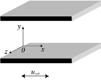
4.1.One dimensional oscillatory Couette flow
We first validate the BLB (JLI, SUS+HS) algorithm by simulating the 1-D oscillatory
Couette flow in the frequency domain. This flow is driven by two parallel plates separated by
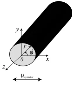
a distance L. The top plate is stationary while the bottom plate oscillates in its own plane with a velocity uwall u e0 i t , where u0 is a constant velocity and
is the radial frequency,see Fig. 1. To characterize the corresponding flow dynamics, we introduce the Stokes number
0 /
S L , with 0 and being the reference density and viscosity of the fluid confined
[image:14.595.213.380.536.673.2]between the plates.
In our simulation, we applied periodic boundary conditions to the two ends in the x
direction, and used the non-equilibrium extrapolation method [43] to prescribe the
perturbation functions on the solid plates subject to no-slip boundary conditions. Moreover,
we specified the sound speed cs 100uwall, and the relaxation time
2
01 c Ss
. To
[image:15.595.75.526.205.560.2]obtain dimensionless numerical results, we chose L1, 0 1 and u0 1.
Fig. 2. Dimensionless streamwise velocities for the oscillatory Couette flows. Open circles: BLB (JLI, SUS+HS) results; Solid lines: analytical solution [32]. (a). S 5; (b). S25; (c).
50
S ; (d). Errors of the LB simulations in different grids when S25.
We performed the BLB (JLI, SUS+HS) simulations on N N 100 100 grids. Fig. 2 shows the dimensionless streamwise velocities (i.e., component in the x direction) for the
flows with S 5, 25 and 50, respectively. In Fig. 2, all velocities include both the real and imaginary parts as these variables are complex-valued in the frequency domain. Interestingly,
have been significantly influenced by oscillatory movement of the bottom plate, see Figs. 2(a)
and 2(b). However, the impact of such a movement becomes rather weak on flow far away
from the plate when the Stokes number grows. This has been clearly exhibited in Fig. 2(c),
where the fluid beyond Y 0.6 is almost unperturbed by the bottom plate’s oscillation. The numerical results in Figs. 2(a) – 2(c) are well agreed with the analytical solutions and the
results given by the TLB simulation [32].
In this numerical case, we also conducted grid-convergence tests of the BLB (JLI,
SUS+HS) algorithm. The oscillatory Couette flow with S =25 was chosen as a test case and
we simulated it using the algorithm on four different grids, i.e., 25 25 , 50 50 , 100 100
and 200 200 . In each grid, we computed the root-mean-square error to quantify the global
accuracy of the LB simulation, i.e.,
20 2
,
1
, m n
m n
x y
E U x y U
N
, (18)where U x
m,yn
and U0 represent the velocity obtained by the LB simulation at the node
xm,yn
and the corresponding analytical solution, respectively. The symbol “” means asum over all nodes in both the x and y directions. Figure 2(d) shows the obtained errors E
in different grids. We see a linear decrease of this error with the increasing grid number in the
double logarithm coordinates. Importantly, the slop of this EN line in Fig. 2(d) is about 2.3. This index evidences that the BLB (JLI, SUS+HS) algorithm proposed in Section 3 is
second-order accurate for the oscillatory Couette flow.
4.2.Two dimensional flow around an oscillating circular cylinder
Next, we apply the BLB (JLI, SUS+HS) algorithm to simulate a 2-D flow generated by
Fig. 3. Schematic of geometry of the flow around an oscillating circular cylinder. Origin of the coordinates system is at the centre of the cylinder.
In this problem, a circular cylinder with a radius a is immersed in a fluid with a density
0
and a viscosity . It oscillates at a horizontal velocity ucylinder u e0 i t parallel to the x
direction [44]. In the corresponding numerical settings, we specified a1, 0 1 and u0 1 to nondimensionalize the results and defined the Stokes number as S 0a2 . The
computational domain was set as a square with a side length L70a. Our numerical tests has validated that this choice is large enough to ensure the fluids far away from the
oscillating cylinder are unperturbed. In this problem, we realized the non-equilibrium
extrapolation scheme [43] was inapplicable in Cartesian coordinates as the treatments set in
this scheme for curved boundaries in rectilinear grids (i.e., lattices) were formulated under
the TLB framework. To circumvent this barrier, we transformed our BLB (JLI, HS+SUS)
simulations to the polar coordinates, which enable the first layer of grid nodes in the radial
direction to be exactly allocated on the cylinder’s surface. With this simple mathematical
manipulation, the non-equilibrium extrapolation scheme [43] becomes workable again in our
simulation. Importantly, the linear LB equation in Section 2 is almost unchanged in the new
coordinates except that the involved spatial gradients turn to
j j j j
j jr
h h c h
c
r r
c
r , (19)
where r and denotes the radial and azimuth coordinates of the polar coordinate system,
HS were carried out for its physical-space discretization on different nodes. The resulting
difference approximations, taking the r direction as example, are
2
( , )
3 , 4 , ,
2
jr jr
m n
j m n j m e n j m e n
j
jr r
h r h r h r
h
e
r r
, (20a)
for bulk nodes while on nodes next to solid boundaries, we have
( , )
, , ,
1 1
2 2
jr jr
m n
j m e n j m n j m e n
j
jr r
h r h r h r
h
e
r r r r
. (20b)
jr
e is the component of ejin the r direction.
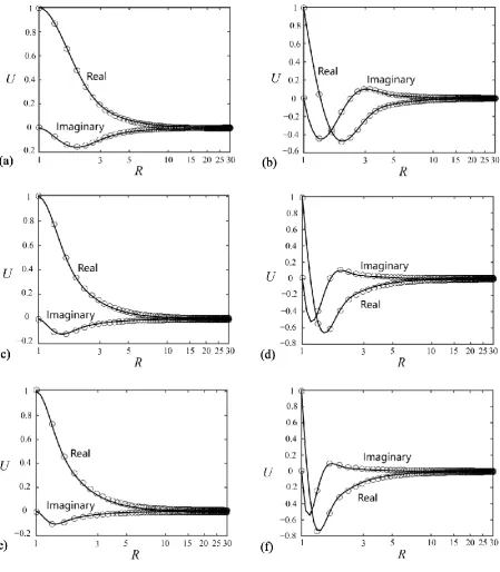
Fig. 4. Dimensionless streamwise velocities for the flow around an oscillating circular cylinder. Open circles: BLB (JLI, HS+SUS) results; Solid lines: analytical solution [44, 45].
(a). S5, 0; (b). S 5, 2; (c). S 25, 0; (d). S25, 2; (e).
50, 0
S ; (f). S50, 2.
illustration, Fig. 4 only exhibits the velocities between R1 and R30 (where R r a) as
the fluids in the region R30 are almost unperturbed to the cylinder’s oscillation. In all cases in Fig. 4, the velocity profiles display significant variations in a boundary layer near the
cylinder’s surface, and then decay to a unperturbed state, i.e., U 0, with the increasing R.
Importantly, we observe that the decay rates of velocities vary with different Stokes numbers:
the velocities at both 0 and 2 corresponding to a larger Stokes number always decay more quickly than those with a smaller S, see Figs. 4(e) and 4(f) in comparison to Figs. 4(a) and 4(b). Theoretically, the Stokes number is a squared ratio of the radius of cylinder to the
viscous penetration depth; the latter is a length scale characterising the velocity decay from
solid boundaries. Therefore, a larger Stokes number implies a shorter viscous penetration
depth for a given cylinder’s radius. This explains the phenomena in Figs. 4(e) and 4(f) that
the velocity profiles have a faster decay rate than those in Figs. 4(a) and 4(b). In addition, we
compared the numerical results with the available analytical solutions [44, 45] for each case
[image:20.595.168.397.390.560.2]in Fig. 4. Again, good agreements between the numerical and analytical results are found.
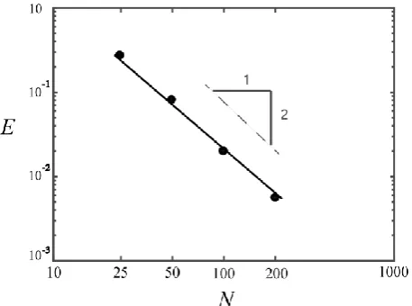
Fig. 5. Comparison of the BLB (JLI, HS+SUS) errors in different grids when S 25, 0.
Our discussion in this simulation also includes grid-dependence tests of the BLB (JLI,
HS+SUS) simulation to quantify its accuracy. We chose25 25 ,50 50 , 100 100 and
200 200 grids to repeat the numerical simulations with S 25, 0. Figure 5 displays the
errors E defined by Eq. (18) in these four grids. As expected, such an error gradually
decreases when denser grids are employed, and the corresponding decreasing slop is 1.9 in
BLB (JLI, HS+SUS) algorithm is nearly second-order accurate for linear oscillatory flow,
regardless of solid boundaries being flat or curved.
4.3.Comparison of computational efficiency
In subsections 4.1 and 4.2, we examined numerical accuracy of the BLB (JLI, HS+SUS)
algorithm. The results demonstrate its high accuracy for simulating linear oscillatory flow.
Examination of its computational efficiency will be conducted in this subsection, especially
in comparison to that of the TLB algorithm constructed with a virtual time scale [32]. We
point out that all simulations in this subsection were performed on the same computer, i.e.,
Dell Precision 7910 CTO.
For simplicity while without loss of generality, we took the 1-D oscillatory Couette flow
with S10 as a test case and recorded the root-mean-square errors E at every 10000 iterative (time) steps for both the BLB (JLI, HS+SUS) and TLB simulations. The decay of
the error is used as a measure to quantify computational efficiency of these LB algorithms.
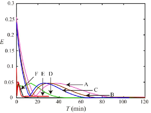
Figure 6 exhibits the root-mean-square errors E during the iterative course in the BLB (JLI,
HS+SUS) simulation (i.e., Curve A) and the time evolution and TLB simulation (i.e. Curve F)
on the 100 100 uniform grids. Interestingly, we see that the TLB algorithm displays a much
faster decay rate (i.e., higher efficiency) than the BLB (JLI, HS+SUS) algorithm. To be
specific, the TLB simulation only spent 12 minutes in reducing its error to 3
1.7 10
E , whereas the time for the BLB (JLI, HS+SUS) algorithm reaching the same error level was
100 minutes. This comparison of E illustrates that as far as computational efficiency is concerned, the BLB (JLI, HS+SUS) algorithm is not a better numerical solver for linear
oscillatory flow. We attribute this inefficiency to the used JLI and motivate a series of
modifications of the proposed BLB algorithm through use of more efficient iterative
approaches and simpler finite difference schemes. To achieve improved computational
efficiency, use of non-uniform grids was also attempted.
Figure 6 shows the error decay of the four BLB algorithms after our modification. Curve
B corresponds to a BLB algorithm still based on JLI but using the HS to approximate all
spatial gradients. Curve C is obtained by the similar algorithm as that for Curve B, but
replacing the JLI by the SLI (see Appendix A for the SLI details). The modified BLB
algorithms for Curve D and E are two versions modified by a combined iterative rule based
details) and 20 100 non-uniform grids, respectively. For convenience, these four modified
BLB algorithms are simply represented as BLB (JLI, HS), BLB (SLI, HS), BLB
[image:22.595.169.430.154.349.2](SLI+ADI+OR, HS) and BLB _N (SLI+ADI+OR, HS) in the next discussion.
Fig. 6. Error decay of different LB algorithms. A: BLB (JLI, SUS+HS); B: BLB (JLI, HS); C: BLB (SLI, HS); D. BLB (SLI+ADI+OR, HS); E: BLB_N (SLI+ADI+OR, HS); F: TLB [32].
In Fig. 6, we compared Curve A with Curve B, and found the use of the HS throughout
in the BLB simulation did not bring about instability, but an improvement in computational
efficiency. As shown by Curve B, the BLB (JLI, HS) algorithm only spent 73.2 minutes to
achieve E1.7 10 3. Such an efficiency improvement is enhanced in the BLB (SLI, HS) simulation. Curve C shows that the change from the JLI to SLI saves about 13.46% in
computational time as compared to Curve B. Meanwhile, however, we also note that the
modifications resulted from the HS and SLI are insufficient – the error-decay rates in Curve
B and Curve C are still far behind that in Curve F (TLB algorithm). This motivates
development of the BLB (SLI+ADI+OR, HS) algorithm and its non-uniform grid version,
i.e., BLB_N (SLI+ADI+OR, HS) algorithm. In these two algorithms, CTDMA (see Appendix
D for the details) was introduced as the replacement of TDMA for direct computation of the
discrete perturbation functions in rows. These functions are subject to periodic boundary
conditions in the oscillatory Couette flow. The error changes of the BLB (SLI+ADI+OR, HS)
and BLB_N (SLI+ADI+OR, HS) simulations are exhibited in Fig. 6, see Curve D and Curve
E. Impressively, unlike those shown in Curve A, Curve B and Curve C, these two
quickly with the progress of computation. In Fig. 6, Curve E is very close to Curve F,
indicating the BLB_N (SLI+ADI+OR, HS) algorithm converged at a comparable rate to that
of the TLB algorithm.
In this subsection, our numerical simulations show the conventional TLB algorithm
exhibits quite good efficiency in comparison to the BLB (JLI, SUS+HS) algorithm and even
some modified BLB algorithms. Only the BLB_N (SLI+ADI+OR, HS) algorithm in our test
has achieved a close convergence rate to the TLB algorithm. For the proposed BLB
simulation, we understand that an appropriate algorithm design is of critical importance for
achieving high computational efficiency. Meanwhile, the BLB algorithm also manifests
distinct numerical compatibility with a large variety of CFD techniques and flexible
applicability in both uniform and non-uniform grids.
5. Conclusion
In this article, we propose a block iterative algorithm to solve the purely
frequency-dependent linear LB model for simulating linear oscillatory flow. The primary feature of this
BLB algorithm, in contrast to the conventional TLB algorithm, is that it completely excludes
any time scale, and computes the perturbation functions directly in the frequency domain
without mimicking a false evolution in virtual time.
Numerical accuracy of the BLB algorithm proposed in this article was validated by
simulating two classical flow problems: the oscillatory Couette flow and flow around an
oscillating circular cylinder with different Stokes numbers. All results are of near
second-order accuracy and well agreed with the available analytical solutions. We also studied
computational efficiency of the BLB algorithm, in particular in comparison to the
conventional TLB algorithm based on the virtual time. A set of modified BLB algorithms
were also proposed and involved in this efficiency comparison. Our simulations reveal that
different BLB algorithms have rather various computational efficiency; only well-designed
BLB version can achieve good efficiency as compared with the TLB algorithm. On the other
hand, our studies also reveals that flexibility and richness in the construction of BLB
algorithms, which is in sharp contrast to its TLB counterpart. The BLB framework can
readily develop various versions through use of different CFD numerical techniques and
grids. This is of value for simulating flow processes in practical M/NEMS, where complex
structures and varying operating conditions are involved. We will investigate such possible
Acknowledgements
The authors would like to acknowledge support from Zhejiang Provincial Natural Science
Foundation of China under Grant No. LY16E060001, Ningbo Science and Technology
Bureau Technology Innovation Team under Grant No. 2016B10010 and Ningbo
International Cooperation Program under Grant No. 2015D10018. Y.S. thanks John E. Sader
for many interesting and stimulating discussions. H.K. acknowledges partial support by
International Doctoral Innovation Centre at the University of Nottingham Ningbo China.
Appendix A. Seidel line iteration
The difference algebraic equations in Section 3, Eqs. (12) and (16), are constructed based
on the JLI, which suffer from low computational efficiency in comparison to the TLB
algorithm. As a solution, we reformulated these equations through use of the SLI.
The major difference of a SLI from a JLI is the former makes use of the latest perturbation
functions on neighbouring nodes for calculation. These latest neighbouring results are
specified at either the
k1
th or kth step, depending on the sweeping direction in which the iteration proceeds. In this appendix, we introduce the SLI-related details used in the BLB(SLI, HS) algorithm in Section 4.3, where spatial gradients on all nodes are approximated by
the HS. Its difference equations after the finite difference discretization are
1 1
+
jy jy
jx jx
s k k k
j j m n j j m n e j j m n e
k s k s k
j m n j j m e n j j m e n
h x , y h x , y h x , y
x , y h x , y h x , y
for ejx 0, (A1)
while
1 1
=
jy jy
jx jx
s k k k
j j m n j j m n e j j m n e
k s k s k
j m n j j m e n j j m e n
h x , y h x , y h x , y
x , y h x , y h x , y
for ejx 0, (A2)
* 1 jy jx s j e e c y x
, (A3)
1
2 jx s j c e x
, (A4)
1
2 jx s j c e x
, (A5)
and j, j and
1 ,
k
j xm ym
are given by Eqs. (17d) – (17f), respectively.
In the BLB (SLI, HS) algorithm, we performed a SLI along the x direction sweeping
from x0 to xN, where x0 xN. Therefore, the three terms on the right hand side of Eqs. (A1)
and (A2) have been specified. In simulation, we applied the TDMA to solve Eqs. (A1) and
(A2) for hkj
x , ym n
,
jy kj m n e
h x , y ,
jy k
j m n e
h x , y and other perturbation functions in the
same column atxxm, and then repeated this direct-solving procedure column by column until the SLI had swept the entire computational domain at the th
k iteration. Generally, our
BLB (SLI, HS) algorithm will terminate its computation once a predefined convergence
criterion is met.
Appendix B. Alternative direction iteration
On top of the SLI, the ADI is another advanced iterative method employed for modifying
the BLB algorithm in Section 4.3. An ADI process designs an iteration consisting of two
successive sweeping– one by columns (along the x direction) and the other by rows (along
the y direction). In this appendix, we discuss the ADI details pertinent to the BLB (SLI+ADI+OR, HS) algorithm.
In the BLB (SLI+ADI+OR, HS) algorithm, a SLI was first conducted along the positive
x direction. The difference algebraic equations in this half are
1 2 1 2 1 2
1 1 2 1
jy jy
jx jx
s k k k
j j m n j j m n e j j m n e
k s k s k
j m n j j m e n j j m e n
h x , y h x , y h x , y
x , y h x , y h x , y
for
0
jx
e , (B1)
1 2 1 2 1 2
1 1 1 2
jy jy
jx jx
s k k k
j j m n j j m n e j j m n e
k s k s k
j m n j j m e n j j m e n
h x , y h x , y h x , y
x , y h x , y h x , y
for ejx 0,(B2)
where the coefficients are defined the same as those in Appendix A. Actually, Eqs. (B1) and
(B2) are almost the same as Eqs. (A1) and (A2) except that the superscript “k” has been
replaced by “
k1 2
” to denote the column sweeping as the first half in one ADI process.Equations (B1) and (B2) were then solved directly using the TDMA following the same
procedure as Appendix A.
Next, the perturbation functions updated by the column sweeping were used as inputs for
the row sweeping along the positive y direction, the second half. The corresponding
difference algebraic equations are
1 2 1 2
jx jx
jy jy
s k s k s k
j j m n j j m e n j j m e n
k k k
j m n j j m n e j j m n e
h x , y h x , y h x , y
x , y h x , y h x , y
for ejy 0, (B3)
while
1 2 1 2
=
jx jx
jy jy
s k s k s k
j j m n j j m e n j j m e n
k k k
j m n j j m n e j j m n e
h x , y h x , y h x , y
x , y h x , y h x , y
for ejy <0.(B4)
Again, the coefficients in Eqs. (B3) and (B4) are the same as those in those in Appendix A
and the terms in the right hand side are all known. We solved Eqs. (B3) and (B4) for the
perturbation functions in the row at y yn by the CTDMA (see Appendix D) as periodic boundary conditions were imposed in the x direction in the oscillatory Couette flow.
With a column sweeping (Eqs. (B1) and (B2)) and a row sweeping (Eqs. (B3) and (B4)),
an ADI process completed updating all perturbation functions in the domain at the kth step.
In the BLB (SLI+ADI+OR, HS) algorithm, we repeated this ADI until convergence was
Appendix C. Over relaxation scheme
The over relaxation (OR) scheme is a simple while efficient means to improve
computational efficiency. In Section 4.3, we applied OR in both the BLB (SLI+ADI+OR, HS)
and BLB_N (SLI+ADI+OR, HS) algorithms.
Consider a perturbation function hkj
x , ym n
, which is just calculated after the TDMA orCTDMA at the th
k step. In the OR framework, the true value of this function will be
modified by
1
1
k k k
j m n o j m n o j m n
h x , y h x , y h x , y , (C1)
where 0 is a numerical weight, and hkj1
x , ym n
is the value of this perturbation functionobtained by the OR at the previous
k1
th step. In Section 4.3, the BLB (SLI+ADI+OR, HS) algorithm chose 0 1.9 in its OR adjustment while 0 1.5 was used in the non-uniform grid version, i.e., the BLB_N (SLI+ADI+OR, HS) algorithm.Appendix D. Cyclic tri-diagonal matrix algorithm
The CTDMA is a variant of the TDMA for a problem with periodic boundary conditions.
As discussed in Section 4.3 and Appendix B, this is the case when we solve the perturbation
functions in one row for the oscillatory Couette flow. Since we only adopted the CTDMA in
the row sweeping in the ADI, we take Eqs. (B3) and (B4) on a row
xx x1, 2,...,xm,...,xN1,xN and y yn
as an example to elaborate its details in this appendix. In the CTDMA framework, Eqs. (B3) and (B4) are rewritten as
x
j
k k k k k k
j m n j m n j m e n j m n j N n j m n
h x , y p x , y h x , y o x , y h x , y q x , y , (D1)
where
1
j k
j m n s k
j j j m n
p x , y
p x , y
, with
1
k s
j n j j
1
k
j j m n
k
j m n s k
j j j m n
o x , y o x , y
p x , y
, with
1
k s
j n j j
o x , y , (D3)
1
1
1, ,
k k
j m n j j m n
k
j m n s k
j j j m n
x , y q x y
q x , y
p x y
, with
1
1 1
k k s
j n j n j
q x , y x , y . (D4)
In Eqs. (D2) – (D4), j max
ejx, 0
c ejx sjx
, max
, 0
jx s
j j jx
c e e
x
and
1 1/ 2 1/ 2
n , jy jy
k k k k
j x , ym j xm yn jhj x , ym n e jhj x , ym n e
, for ejy 0, (D5)
while
1 1/ 2 1/ 2
n , jy jy
k k k k
j x , ym j xm yn jhj x , ym n e jhj x , ym n e
, for ejy 0. (D6)
We point out that different from Eq. (14) in the TDMA, Eq. (D1) includes hkj
x , yN n
when calculating hkj
x , ym n
. This function should be first specified by
1
1
1
1 1 1 1
, ,
,
k k k
j N n j N n j j N n
k
j N n k k k k
j N n j N n j j N n j N n
x y x y q x , y
h x , y
x , y x y p x , y o x , y
r q
p q . (D7)
Equation (D7) includes three new coefficients, pkj , qkj and r jk , and they are computed by a
set of back-substitution equations:
,
1,
1,
1,
k k k k
j xm yn j xm yn j xm yn oj xm yn
r r q , with
1,
k s
j x yn j
r , (D8)
,
1,
1,
k k k
j xm yn j xm yn pj xm yn
![Fig. 2. Dimensionless streamwise velocities for the oscillatory Couette flows. Open circles: BLB (JLI, SUS+HS) results; Solid lines: analytical solution [32]](https://thumb-us.123doks.com/thumbv2/123dok_us/8576035.369141/15.595.75.526.205.560/dimensionless-streamwise-velocities-oscillatory-couette-circles-analytical-solution.webp)