DIFFUSE-INTERFACE TWO-PHASE FLOW MODELS WITH DIFFERENT DENSITIES: A NEW QUASI-INCOMPRESSIBLE
FORM AND A LINEAR ENERGY-STABLE METHOD
M. Shokrpour Roudbaria,†, G. S¸im¸seka,‡,∗, E.H. van Brummelena,§, and K.G. van der Zeeb,∗ aEindhoven University of Technology, Multiscale Engineering Fluid Dynamics,
5600 MB, Eindhoven, Netherlands
†[email protected],‡[email protected],§[email protected]
bThe University of Nottingham, School of Mathematical Sciences, University Park, Nottingham, NG7 2RD, United Kingdom
Received (Day Month Year) Revised (Day Month Year) Communicated by (xxxxxxxxxx)
While various phase-field models have recently appeared for two-phase fluids with dif-ferent densities, only some are known to be thermodynamically consistent, and practi-cal stable schemes for their numeripracti-cal simulation are lacking. In this paper, we derive a new form of thermodynamically-consistent quasi-incompressible diffuse-interface Navier– Stokes Cahn–Hilliard model for a two-phase flow of incompressible fluids with different densities. The derivation is based on mixture theory by invoking the second law of ther-modynamics and Coleman–Noll procedure. We also demonstrate that our model and some of the existing models are equivalent and we provide a unification between them. In addition, we develop a linear and energy-stable time-integration scheme for the de-rived model. Such a linearly-implicit scheme is nontrivial, because it has to suitably deal with all nonlinear terms, in particular those involving the density. Our proposed scheme is the first linear method for quasi-incompressible two-phase flows with nonsolenoidal ve-locity that satisfies discrete energy dissipation independent of the time-step size, provided that the mixture density remains positive. The scheme also preserves mass. Numerical experiments verify the suitability of the scheme for two-phase flow applications with high density ratios using large time steps by considering the coalescence and break-up dynamics of droplets including pinching due to gravity.
Keywords: Navier–Stokes Cahn–Hilliard; quasi-incompressible two-phase-flow; mixture theory; thermodynamic consistency; diffuse interface; energy-stable scheme
AMS Subject Classification: 22E46, 53C35, 57S20
∗Corresponding author
1. Introduction
Diffuse-interface (phase-field) models have emerged as a reliable and versatile alter-native to sharp-interface methods for multi-phase flows. The main idea of diffuse-interface models is to replace the sharp diffuse-interface by a thin, but finite, transition region, where a partial mixing of macroscopically immiscible fluids is allowed, and to define a continuous order parameter (the phase variable) using mass or vol-ume concentration. This leads to the main advantage of diffuse-interface models, which is the natural capability of capturing topological changes, e.g., break-up and coalescence. Another fundamental feature of diffuse-interface models is their rig-orous thermodynamic basis. Most of the models satisfy a nonlinear stability re-lationship such as dissipation of a non-convex free-energy functional, which en-dows these models with a strong mathematical foundation. Over the years, dif-fuse interface models have been analyzed theoretically16,17,28,1 and used widely in many applications5,11,40,45,54, while several reviews4,25,38 have appeared of phase-field models in the context of fluid mechanics.
In this work we derive a new form of diffuse-interface model, and a corresponding practical time-stepping method, for binary-fluid flows whose components are incom-pressible with different densities. The model is a so-called quasi-incompressible43 Navier–Stokes-Cahn–Hilliard (NSCH) model, which is based on the Navier–Stokes equations coupled with the convective Cahn–Hilliard equation. The Cahn–Hilliard equation is a fundamental continuum model for phase separation individually, which was introduced by Cahn & Hilliard12in 1958. Since it is a fourth-order singularly-perturbed nonlinear parabolic PDE, it is challenging to solve it numerically. Cou-pling it with the Navier–Stokes equations increases the mathematical complexity of the model which makes it difficult to design provably stable numerical schemes. We will introduce a linear and stable time-integration scheme for our derived quasi-incompressible NSCH model. The scheme preserves the structural properties of the model, viz. mass conservation and energy dissipation, at the semi-discrete level independent of the time-step size.
withnon-matching component densities.
Lowengrub & Truskinovsky43 and Abels, Garcke & Gr¨un2 extended Model H to thermodynamically-consistent models fornon-matching densities using two dif-ferent modelling assumptions on the velocity field (mass averaged and volume av-eraged velocity, respectively) and on the phase-field variable (mass concentration and volume fraction, respectively). Although the models by Lowengrub & Truski-novsky and Abelset al.are developed to represent the same type of flow dynamics, the resulting equations have significant differences due to the underlying modeling choices. More precisely, by adopting a mass-averaged mixture velocity, the model by Lowengrub & Truskinovsky (see also Kim & Lowengrub40) leads to a (generally) non-solenoidal velocity field (divv6= 0) and additional nonlinear terms compared to Model H, whereas the volume-averaged mixture-velocity model of Abels et al. has a solenoidal velocity field and a modified momentum equation (similar to an earlier model obtained by Boyer10 through asymptotic arguments).
Noteworthy are also the recent follow-up works by Shen, Yang & Wang49 and Aki, Dreyer, Giesselmann & Kraus3, who independently introduced seemingly dif-ferent quasi-incompressible NSCH models based on a volume-fraction phase vari-able and non-solenoidal mass-averaged velocity. Shen et al. obtained their model without reference to a Coleman–Noll procedure, but were able to demonstrate global energy dissipation for their model. The work of Aki et al.actually contains the derivation of a more general Navier–Stokes–Korteweg/Cahn–Hilliard/Allen– Cahn model in the non-isothermal and isothermal case (and also includes phase transition). Their derivation leads to a Korteweg stress tensor term as commonly seen in Navier–Stokes–Korteweg models4,32,42,25,21. Other simpler models have also been introduced,15,47,11 which neglect certain terms in the above-mentioned quasi-incompressible models. These models seem to beinconsistent with mixture theory and the second law of thermodynamics, and have been studied mostly because of their simpler implied numerical treatment, which is closer to that of the variable-density Navier–Stokes equations26and Volume-of-fluid (VOF) method46.
The first objective of this paper is to derive from mixture theory the following new form of quasi-incompressible NSCH model:
˙
φ+φ∇ ·v=∇ ·(m(φ)∇µ) µ= σ
df
dφ−σε∆φ− p
ˆ ρ
dˆρ dφ
ρv˙ =−∇p−φ∇µ+p ˆ ρ
dˆρ
dφ∇φ+∇ · η(φ)(2D+λ(∇ ·v)I)
−ρgˆ
∇ ·v=α∇ ·(m(φ)∇µ) ˙
ρ+ρ∇ ·v= 0 ˆ
ρ=ρ11 +φ 2 +ρ2
1−φ 2
(1.1)
the pressure and ρ= ˆρ≡ρ(φ) is the mixture density. Moreover,ˆ ρ1 andρ2 are the component densities (assumed constant), σ is a constant related to the fluid-fluid surface tension,εis the interface thickness parameter,η(φ) is the mixture viscosity, m(φ) is a mobility function,α= ρ2ρ2−+ρ1ρ1 is a constant, and λ≥ −2/d is a constant (d being the dimension). Furthermore, the term ˆρg stands for the gravitational force and D is the symmetric velocity gradient tensor. Note that we presented model (1.1) with a compatible dual-density form, viz.ρand ˆρ. The appearance of two equivalent but distinct representations of the mixture density specifically serves in the construction of a linear energy-stable time-integration scheme; see below.
The distinguishing feature of model (1.1) is the term pρˆddφρˆ (in (1.1)2and (1.1)3), which has not appeared in previous quasi-incompressible NSCH models. We will show that our model is nevertheless equivalent to the model by Shen, Yang and Wang49, as well as the corresponding model in Aki, Dreyer, Giesselmann and Kraus3. We thereby provide a unification of the existing models based on a mass-averaged velocity and volume-fraction phase variable. It should be noted that in the case of matching densities, all of the aforementioned NSCH models for variable-density two-phase flows, including our model, reduce to Model H.
The development of stable and efficient time-integration methods for NSCH sys-tems with non-matched densities is challenging on account of the strong coupling between the equations and the various nonlinear terms, in particular those involv-ing the density. An important notion in the analysis of stability of time-integration schemes is that ofenergy stability, which implies that the discrete time-integration scheme inherits the fundamental free-energy dissipation property of the underly-ing PDE system.18,25 Unconditional energy stability is crucial for robustness of diffuse-interface simulations and for proper resolution of interfaces as it enables, in principle, arbitrary time and space discretizations and hence provides a basis for adaptive refinement.
In the case of the Cahn–Hilliard equation, various energy-stable semi-discrete (continuous in space, discrete in time) schemes of first and second order have ap-peared over the past years,57,35,24,52,59,25 some of which are linear, i.e., they re-quire only one solution of a linear-algebraic system per time step.a These schemes have been extended to NSCH systems with matched densities39,31 and for quasi-incompressible NSCH systems with a solenoidal mixture-velocity field15,47,44,48,22. However, non-solenoidal quasi-incompressible NSCH systems have only received scant consideration so far. The reason for this is that existing techniques for solenoidal systems can not be straightforwardly extended to non-solenoidal sys-tems (which apart from being non-solenoidal also have auxiliary pressure terms). One recent scheme is by Guo, Lin & Lowengrub27, who proposed a complicated nonlinear energy-stable scheme for the model by Lowengrub & Truskinovsky43.
The second objective of this work is to introduce a simplelinear energy-stable
aLinear energy-stable schemes typically require that the nonconvex free energy has quadratic
time-integration scheme for model (1.1). The proposed scheme is energy stable in-dependent of the time-step size, provided that the mixture density remains positive. Moreover, under standard assumptions on the boundary conditions, the scheme is mass conservative. To our knowledge, this is the first work with a linear energy-stable time-integration scheme for a quasi-incompressible NSCH system with non-solenoidal velocity field. In contrast to existing time-integration schemes, we make use of a dual-density formulation involving both ρ and ˆρin its discretization (see Section 3.2). The dual-density formulation provides the basis for the energy stability of the scheme, especially for numerical computations with high component-density ratios.
The remainder of this paper is structured as follows: In Section 2, we derive the new form of thermodynamically consistent quasi-incompressible model for two-phase flows and discuss its equivalence to other models. Section 3 presents a weak form of the system and a time-discrete scheme including proofs of continuous and discrete energy dissipation. In Section 4, we exhibit the properties of our fully-discrete scheme based on numerical computations using standard finite elements as a spatial discretization. Section 5 presents concluding remarks.
2. Derivation of the Quasi-Incompressible NSCH Model
In this section, we present a new form of quasi-incompressible diffuse–interface NSCH model with gravity, inspired by Aki, Dreyer, Giesselmann and Kraus3. We derive the model for an isothermal mixture with a thin interfacial region between two immiscible and incompressible fluids. The derivation is based on the theory of mixtures9,53, which assumes that the mass, momentum and energy are conserved at the constituent level as well as within the mixture, see Sections 2.1–2.3. The model is derived in Sections 2.4–2.5 via application of the standard Coleman–Noll procedure13,29 to the energy dissipation inequality, which enforces the second law of thermodynamics and endows the model with thermodynamic consistency. We demonstrate the equivalence of the model to other existing models in Section 2.6, and present a non-dimensionalisation and interface-profile analysis in Sections 2.7– 2.8.
2.1. Continuum theory of mixtures
To provide a setting for our model, we consider an open bounded domain Ω⊂Rd
(d = 2,3) and label the fluids of the binary mixture by k = 1,2. Let the volume fractionb be φk =Vk/V, where Vk is the volume of thekth component and V is
as ck = Mk/M with the mass of the kth component, Mk, and the total mass
of the mixture, M. Particularly, since M = P
kMk and V = PkVk, we have P
kck =Pkφk = 1.
Each component of the fluid is assumed to be incompressible, so we describe a constant specific densityρk =Mk/Vk fork= 1,2. Similarly,partial mass densities
can be defined as ˜ρk =Mk/V, which arenon-constant and their sum is the total
mass density of the mixture, ρ=P
kρ˜k. Note that the three densities are related
by
˜
ρk=ρkφk=ρck. (2.1)
Unlike the individual components, the mixture is not assumed to be incompress-ible. We assume the mixture density to be a function of an order parameterφsuch thatρ≡ρ(φ), whereˆ φis related to the volume fractions according toφ:=φ1−φ2. It is to be noted that the total density can generally be chosen as a function of various combinations of volume or mass fractions, some of which are mentioned by Abels, Garcke & Gr¨un2. We define the order parameter φ based on the volumes V1, V2 and V by V1/V = (1 +φ)/2 and V2/V = (1−φ)/2, which leads to the relations ˜ρ1 =ρ1(1 +φ)/2 and ˜ρ2 =ρ2(1−φ)/2, forφ∈[−1,1]. This implies the following algebraic equation for the mixture density:
˜
ρ1+ ˜ρ2=ρ1 1 +φ
2 +ρ2 1−φ
2 =: ˆρ(φ). (2.2)
Note that ˆρ(φ) coincides with the mixture densityρ, where both represent the non-constant mixture density. Although ρand ˆρ:= ˆρ(φ) coincide, they serve separate roles in the formulation and, accordingly, can not be used interchangeably. We introduce the mixture velocityvas themass averaged/barycentric velocity:
v=1 ρ
X
k
˜
ρkvk, (2.3)
wherevk denotes the velocity of componentk.
2.2. Balance equations
Balance of mass for the individual constituentsk= 1,2 can be written as
∂tρ˜k+∇ ·( ˜ρkvk) = 0, (2.4)
where we assume no mass production of or conversion between the constituents, which is reflected in the zero right hand side.
We replace ˜ρ1and ˜ρ2 byρ1(1 +φ)/2 and ρ2(1−φ)/2 in (2.4), respectively, use the definition of diffusion velocity according to wk =vk−v and relation (2.1) to
obtain
∂t ρ1
2 (1 +φ)
+∇ ·ρ1
2 (1 +φ)v
+∇ ·( ˜ρ1w1) = 0 (2.5) ∂t
ρ2
2 (1−φ)
+∇ ·ρ2
2 (1−φ)v
Multiplying (2.5) and (2.6) by 1/ρ1 and 1/ρ2, respectively, and subtracting the resulting equations gives the phase equation:
˙
φ+φ∇ ·v+∇ ·h= 0 (2.7)
where h = φ1w1−φ2w2 is the mass flux due to diffusive changes in the phase variableφand ˙xis the material derivative ˙x=∂tx+v· ∇xfor any field variablex.
Similarly, summing the equations in (2.5)–(2.6) and using the identityρ1φ1w1+ ρ2φ2w2 = 0, which can be inferred from (2.3), we obtain the following quasi-incompressibility relation for the mixture velocityv:
∇ ·v+α∇ ·h= 0, (2.8)
where
α:=ρ2−ρ1
ρ2+ρ1 (2.9)
is a constant. By combining (2.7) and (2.8) we obtain the following relation between the phase variable and the mixture velocity:
∇ ·v= α 1−αφ
˙
φ. (2.10)
Remark 2.1. If the specific densities are equal, that is,ρ1=ρ2, then (2.8) reduces to∇ ·v= 0. The barycentric velocity is therefore solenoidal if the specific densities of the two components coincide, but not generally otherwise.
Balance of mass is not only satisfied for the components, but also for the mixture. Indeed, summing (2.4) ink, we obtain
∂tρ+∇ ·(ρv) = 0 or ρ˙+ρ∇ ·v= 0 (2.11)
and similarly
∂tρˆ+∇ ·( ˆρv) = 0, (2.12)
where ˆρ is the algebraic definition of the mixture density as in (2.2). Then, from (2.12) it follows that
∇ ·v=−1
ˆ ρρ˙ˆ=−
1 ˆ ρ
dˆρ dφ ˙
φ, (2.13)
which is another identity for the divergence of the mixture velocity in (2.8). Addi-tionally, from (2.10) and (2.13), we have
−1
ˆ ρ
dˆρ dφ=
α
1−αφ, (2.14)
For our model, we are interested in the velocity of the mixture,v, more than the specific velocities,vk. Therefore, instead of introducing the momentum equation for
each constituent, we will consider the mixture momentum balance ∂t(ρv) +∇ ·(ρv⊗v) =∇ ·T+b,
whereTis the stress tensor of the mixture andbis the body force. By (2.11), this can be simplified to
ρv˙ =∇ ·T+b. (2.15)
We restrict our considerations here to body-force terms corresponding to gravita-tional effects. Accordingly,bin (2.15) is replaced by−ρgˆ with g as gravitational acceleration andas the vertical unit vector.
Remark 2.2. An alternative mixture velocity definition to (2.3) is the volume-averaged velocityv =φ1v1+φ2v2, which is employed in other works2,10,22. This choice would reduce (2.8) to ∇ ·v = 0 even for non-matching densities, i.e. for ρ16=ρ2. However, this simplification requires a change in the conservation equations for mass and momentum to obtain a thermodynamically consistent model. More explicitly, volume averaged velocity leads to an additional term in the momentum conservation equation related to diffusion of components in order to describe the density flux.2
2.3. The second axiom of thermodynamics
Similar to the momentum equation (2.15), we assume the balance of internal energy not for the individual constituents, but for the mixture. However, instead of intro-ducing the balance of energy equation here, we directly consider the second axiom of thermodynamics in the form of an energy dissipation inequality.30 The connection between the internal-energy density and the dissipation inequality is made via the Helmholtz free-energy density,ρψ.
Let us consider the following energy dissipation inequality in terms of the free energy ρψ, the kinetic and gravitational potential energy K(P) and G(P), the total work done by macro- and micro-stressesW(P) and the energy transported by diffusionM(P):
d dt
Z
P(t)
ρψ+K(P) +G(P)dv≤W(P)−M(P), (2.16)
where P denotes any time-dependent subset of Ω, which moves with the mixture velocityv.
and the gravitational potential energy. Specifically, following Gurtin28 we consider K(P) = 1
2ρ|v|
2, G(P) = ˆρgy, (2.17)
W(P) =
Z
∂P
Tn·vda+
Z
∂P
˙
φξ·nda, M(P) =
Z
∂P
µh·nda, (2.18)
whereyis the vertical coordinate,nis the exterior unit normal vector to the bound-ary ofP,∂P, µdenotes a chemical potential and ξis a vectorial surface force as a component of micro-stress.
Upon substituting (2.17) and (2.18) into (2.16) and applying the Reynolds trans-port theorem, we obtain
Z
P
∂
∂t(ρψ)dv+
Z
∂P
ρψv·nda+
Z
P
1 2
∂ ∂t(ρ|v|
2)dv
+
Z
∂P
1 2ρ|v|
2
v·nda+
Z
P
∂tρgy dvˆ + Z
∂P
ˆ
ρgyv·nda
≤ Z
∂P
Tn·vda+
Z
∂P
˙
φξ·nda− Z
∂P
µh·nda.
(2.19)
Then using the conservation laws (2.11), (2.12) and (2.15) on the left hand side and the divergence theorem on the right hand side of the inequality, the following local form of (2.19) is obtained:
ρψ˙−T:∇v− ∇ ·( ˙φξ) +∇ ·(µh)≤0. (2.20) By applying the product rule to the last two terms in (2.20) and introducing
˙
ρψ =ρψ˙+ψρ˙ and T=T0−pI, we obtain
˙
ρψ−ψρ˙−T0:∇v+p∇ ·v−φ˙∇ ·ξ−ξ∇( ˙φ) +µ∇ ·h+h· ∇µ≤0. (2.21) The partition T=T0−pIis such that −pI corresponds to the hydro-static part of the stress tensor T. The reduced dissipation inequality (2.21) forms the basis for determining our class of admissible constitutive relations and the independent variables.
2.4. Constitutive equations and Coleman–Noll procedure
We consider the independent variables: φ,v, µ, p and the dependent functions: ρψ,ρ,ˆ T,h,ξ. The explicit form of the functions in terms of independent variables is determined via the Coleman–Noll procedure, except ˆρwhich has been defined pre-viously in (2.2). We start with the constitutive assumption for the energy density ρψ according toρψ=ρψ(φ,c ∇φ), which gives
˙
c
ρψ=∂(ρψ)c ∂φ
˙
φ+∂(ρψ)c ∂∇φ
˙
∇φ. (2.22)
Furthermore, on account of∇˙φ=∇( ˙φ)− ∇v· ∇φ, it follows from (2.22) that ˙
c
ρψ= ∂(ρψ)c ∂φ
˙
φ+∂(ρψ)c ∂∇φ ∇( ˙φ)−
∂(ρψ)c
∂∇φ ⊗ ∇φ
!
:∇v. (2.23)
Using the identities (2.8), (2.11) and (2.23), the inequality (2.21) can be recast into ∂(ρψ)c
∂φ ˙
φ+∂(ρψ)c
∂∇φ ∇( ˙φ)−
∂(ρψ)c
∂∇φ ⊗ ∇φ
!
:∇v+ (ρψ)c I:∇v−T0:∇v + p∇ ·v −φ˙∇ ·ξ−ξ∇( ˙φ) + µ∇ ·h +h· ∇µ≤0,
(2.24)
where pI: ∇v =p∇ ·v. In (2.24), we have written each term as a contraction of a dependent and an independent variable except for the boxed terms. The boxed terms can be recast into the same form by means of the relations
∇ ·v=−1
ˆ ρ
dˆρ dφ ˙
φ and ∇ ·h=−φ˙−φ∇ ·v, (2.25) which results in the following local dissipation inequality
∂(ρψ)c
∂φ ˙
φ+∂(ρψ)c
∂∇φ ∇( ˙φ)−
∂(ρψ)c
∂∇φ ⊗ ∇φ
!
:∇v+ (ρψ)c I:∇v−T0:∇v
−p
ˆ ρ
dˆρ dφ ˙
φ−φ˙∇ ·ξ−ξ∇( ˙φ) +µ(−φ˙−φ∇ ·v) +h· ∇µ≤0.
(2.26)
ReplacingT0 byT0=T+pIand rearranging terms, we obtain
− ∇v: T+pI+∂(ρψ)c
∂∇φ ⊗ ∇φ+ (µφ−ρψ)c I
!
+ ˙φ ∂(ρψ)c
∂φ − ∇ ·ξ−µ− p ˆ ρ
dˆρ dφ
!
+∇( ˙φ) ∂(ρψ)c ∂∇φ −ξ
!
+h· ∇µ≤0.
Based on the inequality (2.27), we choose the constitutive relations as:
T=Tˆ(φ,∇φ,∇v) ξ= ˆξ(φ,∇φ)
h=ˆh(φ,∇φ, µ,∇µ),
where according to the standard Coleman–Noll argument, the form of the functions can be selected arbitrarily. To avoid that a variation of ˙φ and ∇( ˙φ) leads to a violation of the inequality (2.27), we insist that:
∂(ρψ)c
∂φ − ∇ ·ξ−µ− p ˆ ρ
dˆρ
dφ = 0 (2.28)
∂(ρψ)c
∂∇φ −ξ= 0, (2.29)
which provide equations for µand ξ, respectively. The following constitutive rela-tions then ensure compliance with (2.27):
h=−m(φ)∇µ, (2.30)
T+pI+ ∂(ρψ)c ∂∇φ ⊗ ∇φ
!
+ (µφ−ρψ)c I=η(φ) (2D+λ(∇ ·v)I) (2.31)
where D = 1
2 ∇v+∇v
T
is the symmetric velocity gradient tensor and ∇vT
denotes transpose of∇v. Then (2.27) is satisfied as, in particular,
−η(φ) (2D+λ(∇ ·v)I) :∇v−m(φ)|∇µ|2≤0,
where η(φ)≥0 is the viscosity, m(φ)≥is the mobility. The viscous contribution
−η(φ) (2D+λ(∇ ·v)I) is non-positive under the standing assumptionλ≥ −2/d.51
Remark 2.4. We introduce η(φ) (2D+λ(∇ ·v)I) as the viscous stress tensor where the fluid is considered to be an isotropic Newtonian mixture with volume-fraction-dependent viscosity.45
2.5. Special choice of free energy and the Navier–Stokes Cahn–Hilliard Equation
To obtain a specific quasi-incompressible model, we choose the Helmholtz free en-ergy in the Ginzburg-Landau form12:
c
ρψ(φ,∇φ) = σ εf(φ) +
σε 2 |∇φ|
2,
whereε >0 represents the thickness of the interface of the mixture,σis related to the surface energy density andf(φ) represents a double-well potential, for example the globallyC2,1-continuous standard (truncated) quartic polynomial according to
f(φ) :=
(φ+ 1)2, φ <−1 1
4(φ
2−1)2, φ∈[−1,1] (φ−1)2, φ >1
Then, by the definition ofρψc it holds that
∂(ρψ)c
∂φ = σ ε
df dφ,
∂(ρψ)c
∂∇φ =σε∇φ. (2.33)
If we substitute (2.33) into (2.28)–(2.31) and by (2.7) and (2.15), we obtain the following quasi-incompressible Navier–Stokes-Cahn–Hilliard system:
˙
φ+φ∇ ·v=∇ ·(m(φ)∇µ) (2.34a)
µ= σ
df
dφ−σε∆φ− p ˆ ρ
dˆρ
dφ (2.34b)
ρv˙ =−∇p−σε∇ ·(∇φ⊗ ∇φ) +∇ ·σ
εf(φ) + σε
2 |∇φ| 2
−µφI
+∇ · η(φ) (2D+λ(∇ ·v)I)
−ρgˆ (2.34c)
∇ ·v=α∇ ·(m(φ)∇µ) (2.34d)
˙
ρ+ρ∇ ·v= 0 (2.34e)
ˆ ρ=ρ1
1 +φ 2 +ρ2
1−φ
2 (2.34f)
The NSCH system (2.34) is thermodynamically consistent by construction, i.e. it complies with the second law of thermodynamics.
Remark 2.5. One may note that the two variants (2.34e) and (2.34f) of the mixture density both appear in the equation of motion (2.34c). More explicitly, the density in (2.34e) appears in theρv˙ term, while the density in (2.34f) appears in the gravity term ˆρg. (2.34f) also appears in the equation of chemical potential (2.34b). Defining the mixture densities ρand ˆρvia two separate equations in (2.34e) and (2.34f) is crucial to obtain an energy dissipative time-discrete scheme. These two definitions of the mixture density are consistent by construction; see Section 2.1.
Remark 2.6. The components of the stress in (2.34c) can be endowed with specific physical interpretations. The tensorη(φ)(2D+λ(∇ ·v)I) represents the standard viscous stress tensor. The tensorsσε(∇φ⊗ ∇φ) and σεf(φ) +σε2|∇φ|2−µφ
Iare associated with capillary forces due to the surface tension and an additional contri-bution due to quasi-incompressibility, respectively.
Equation (2.34c) can be reformulated such that the additional complicated stress terms assume a simpler form. To this end, we note that for σε∇ ·(∇φ⊗ ∇φ) we have the following sequence of identities:
σε∇ ·(∇φ⊗ ∇φ) =σε(∆φ∇φ+1 2∇|∇φ|
2) =∇φ
σ ε
df dφ−µ−
p ˆ ρ
dρˆ dφ
+σε 2 ∇|∇φ|
2
=∇ ·σ
εf(φ) + σε
2 |∇φ| 2
−µφI+φ∇µ−p
ˆ ρ
dˆρ
where the second identity in (2.35) follows from (2.34b). Inserting (2.35) into (2.34c) leads to the final form of the quasi-incompressible Navier–Stokes Cahn–Hilliard model
˙
φ+φ∇ ·v=∇ ·(m(φ)∇µ) µ=σ
df
dφ−σε∆φ− p ˆ ρ
dˆρ dφ
ρv˙ =−∇p−φ∇µ+p ˆ ρ
dˆρ
dφ∇φ+∇ ·(η(φ) (2D+λ(∇ ·v)I))−ρgˆ
∇ ·v=α∇ ·(m(φ)∇µ) ˙
ρ+ρ∇ ·v= 0 ˆ
ρ=ρ1 1 +φ
2 +ρ2 1−φ
2
(2.36a) (2.36b) (2.36c) (2.36d) (2.36e) (2.36f)
Remark 2.7. For matching densities, i.e.ρ1=ρ2, equations (2.36e) and (2.36f) are trivially satisfied and equations (2.36a)–(2.36d) reduce to the standard incompress-ible NSCH system30. Additionally, the−φ∇µterm can be rewritten as∇·(∇φ⊗∇φ) upon redefining the pressure by ˜p=p−σ
εf(φ)− σε
2|∇φ| 2+µφ.
In the sequel, we will generally equip (2.36) with the following natural boundary conditions:
∂nφ=∂nµ= 0, v= 0 on∂Ω, (2.37)
where ∂n(·) represents the normal-derivative in the trace sense. Also, for the sake
of simplicity, we restrict our considerations to constant viscosity and mobility, i.e. η(φ) :=η andm(φ) :=m.
Remark 2.8. Other boundary conditions, e.g. of non-homogeneous form can be considered as well. However, one should take into consideration that there is a compatibility between the velocityvand the chemical potentialµdue to the quasi-incompressibility equation (2.36d), that is,
Z
∂Ω
v·ndS=α
Z
∂Ω
m(φ)∂nµ dS
The total energy functional associated with (2.36) is compatible with (2.16) and comprises the Helmholtz free energy, the kinetic energy and the gravitational energy:
E(φ, ρ,ρ,ˆ v) :=
Z
Ω
1
2ρ|v| 2+σ
εf(φ) + σε
2 |∇φ| 2+ ˆρgy
dΩ, (2.38)
Here, 12ρ|v|2is the kinetic energy,σ εf(φ) +
σε
2|∇φ|
2.6. Equivalent form and relation to existing models
Based on the same modeling assumptions, one can derive a seemingly different quasi-incompressible model to (2.36). Let us follow the same steps in the derivation until (2.24) and rewrite the termp∇ ·vusing
∇ ·v=αφ˙+αφ∇ ·v (2.39)
instead of∇ ·v=−1
ˆ ρ
dˆρ dφ ˙
φin (2.25). Then the local dissipation inequality becomes ∂(ρψ)c
∂φ ˙
φ+∂(ρψ)c
∂∇φ ∇( ˙φ)−
∂(ρψ)c
∂∇φ ⊗ ∇φ
!
:∇v+ (ρψ)c I:∇v−T0:∇v +αpφ˙+ (αpφ)I:∇v−φ˙∇ ·ξ−ξ∇( ˙φ) +µ(−φ˙−φ∇ ·v) +h· ∇µ≤0.
(2.40)
Applying the Coleman–Noll procedure to (2.40), we obtain the same equations as (2.29) and (2.30) and the following two equations for chemical potential and the stress tensor:
∂(ρψ)c
∂φ − ∇ ·ξ−µ+αp= 0
T+pI+ (ξ⊗ ∇φ) + (µφ−ρψc+αpφ)I=η(φ) (2D+λ(∇ ·v)I).
(2.41)
Hence, repeating the steps in (2.35), we obtain the following alternative quasi-incompressible NSCH model:
˙
φ+φ∇ ·v=∇ ·(m(φ)∇µ) µ=σ
ε df
dφ−σε∆φ+αp
ρv˙ =−∇p−φ∇(µ−αp) +∇ ·(η(φ) (2D+λ(∇ ·v)I))−ρgˆ
∇ ·v=α∇ ·(m(φ)∇µ) ˙
ρ+ρ∇ ·v= 0 ˆ
ρ=ρ11 +φ 2 +ρ2
1−φ 2 .
(2.42a) (2.42b) (2.42c) (2.42d) (2.42e) (2.42f) It can be observed, however, that the models (2.36) and (2.42) are equivalent, by redefining the pressure! Using the relation (2.14), if the pressure pin (2.42b) and (2.42c) is redefined asp= 1−p˜αφ, then one obtains (2.36b) and (2.36c).
Remark 2.9 (Equivalence with Shen, Yang & Wang). The form obtained in (2.42) is equivalent to the model by Shen, Yang & Wang49, which was derived using different arguments, not invoking the Coleman–Noll procedure. Indeed, their Eqs. (2.13a)–(2.13d) on their page 1050, can be obtained from our (2.42a)–(2.42d) upon simply redefining ourρ2= 2 ˜ρ2−ρ1, to account for the fact that their phase variable ranges from 0 to 1 (as opposed to−1 to 1 in our case). With that substitu-tion, theαin (2.42b)–(2.42d) changes to ρ2˜ρ−˜ρ1
2 , and ˆρ(φ) =ρ1φ+ ˜ρ2(1−φ), which
Remark 2.10 (Equivalence with Aki, Dreyer, Giesselmann & Kraus). The form obtained in (2.42) is also equivalent to the isothermal form (and without phase transition) of the generalized model by Aki, Dreyer, Giesselmann & Kraus3. Indeed, using (2.35) and the identity
∇ ·∇φ⊗ ∇φ−(φ∆φ+12|∇φ|2)I=−φ∇∆φ , Eq. (2.42c) can be written as
ρv˙ =−∇p+σεφ∇∆φ+∇P(φ) +∇ ·(η(φ) (2D+λ(∇ ·v)I))−ρgˆ (2.43) where P(φ) :=φdW
dφ(φ)−W(φ) is the thermodynamic pressure as used by Aki et
al., andW(φ) :=σε−1f(φ). The system given by (2.42a), (2.42b), (2.43), (2.42d) is now exactly equal to the one in Akiet al.on page 828 (cf. their Eqs. (2.16)–(2.20)), upon setting the mobilities in their model tomj= mc(2φ)
+
andmr= 0.
These equivalences unify the seemingly different quasi-incompressible NSCH models based on the mass-averaged velocity and volume-fraction phase variable, which have all been derived in different ways.
2.7. Non-dimensionalization
We perform the non-dimensionalization of (2.36) based on physical properties of the liquid associated with the density ρ1, which are the characteristic scales of length, L∗, velocity,U∗andP∗=σ/L∗. Considering thatφis already a dimensionless phase
field variable, the governing dimensionless variables are given by: ¯
x= x L∗
¯
v= v U∗
¯ t=tL∗
U∗
¯ p= p
P∗
¯ µ= µ
P∗
¯ ρ= ρ
ρ1
whereP∗is used for both dimensionless pressure and chemical potential.
Suppress-ing the over bar for the sake of simplicity, the dimensionless quasi-incompressible NSCH system (2.36) writes as:
˙
φ+φ∇ ·v= 1 Pe4µ µ= 1
Cn df
dφ−Cn∆φ− p
ˆ ρ
dˆρ dφ
ρv˙ =− 1
We
∇p+φ∇µ−p
ˆ ρ
dˆρ dφ∇φ
+ 1
Re∇ ·(2D+λ(∇ ·v)I)− 1 Fr2ρˆ
∇ ·v= α Pe4µ ˙
ρ+ρ∇ ·v= 0 ˆ
ρ= 1 +φ
2 +
ρ2 ρ1
1−φ 2 ,
(2.44a) (2.44b)
where Pe = U∗L2∗/mσ is the diffusional P´ecletnumber, Cn = ε/L∗ is the Cahn
number as a measure of the interface thickness, We = ρ1U∗2L∗/σ is the Weber
number, Re =ρ1U∗L∗/ηis the Reynolds number and Fr =U∗/
√
gL∗ is the Froude
number, which expresses the relative strengths of the inertial and the gravitational forces. Additionally, αis the ratio of specific densities as already defined in (2.9) and the dimensionlessdˆρ/dφwrites:
dˆρ dφ=
1 2
1 +ρ2 ρ1
.
The dimensionless form of (2.42) can be obtained similarly.
In addition to the main system, the dimensionless energy is obtained from (2.38) by rescaling ¯E =E/ρ1U∗2 as
E(φ, ρ,ρ,ˆ v) =
Z
Ω
1
2ρ|v| 2
+ 1
We Cnf(φ) + Cn 2 We|∇φ|
2 + 1
Fr2ρyˆ
dΩ. (2.45)
2.8. Interface profile
To elucidate the manner in which the fluid–fluid interface is represented in the quasi-incompressible NSCH model (2.44), we consider the particular case of a stationary planar fluid–fluid interface in the absence of gravity. Under suitable boundary con-ditions, it follows from (2.44) thatv= 0 andµ= const. Denoting bysa coordinate normal to the interface and centered at the interface, equations (2.44) then imply
dp ds− p ˆ ρ dˆρ dφ dφ ds = 0 µ− 1
Cn df dφ+ Cn
d2φ ds2 +
p ˆ ρ
dρˆ dφ= 0
in R (2.46)
We insist that the mixture reduces to the pure species and exhibits a uniform pressure (i.e. trace of the stress) away from the interface:
lim
s→±∞φ(s) =±1 s→±∞lim dp(s)−trζ(s) =dp∞ (2.47)
whereζ represents the dimensionless capillary-stress tensor according to ζ=−Cn∇φ⊗ ∇φ+I
Cn 2 ∇φ 2 + 1
Cnf(φ)−µφ
=−Cn
2 dφ ds 2 + 1
Cnf(φ)−µφ
(2.48)
and trζ represents its trace. The second identity in (2.48) holds in the one-dimensional case under consideration. The first equation in (2.46) can be solved via separation of variables to obtain the general solutionp=Cρ(φ) for some con-stantC. It can then be verified by substitution that
φ(s) = tanh
s
√
2 Cn
p(s) =p∞+p∞
ρ1−ρ2 ρ1+ρ2
φ(s) µ=−p∞
ρ1−ρ2 ρ1+ρ2
-2 -1 1 2 1
2 3 4
0 0
Cn=2-1
Cn=2-2
Cn=2-3
Cn=20
s
(
)
si
n
h
4
(
)
s
√
2
C
n
1
2
C
n
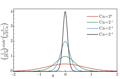
Fig. 1: Illustration of the energy density in (2.50) for Cn∈2{−3,−2,−1,0}.
solves (2.46)–(2.47). It is to be noted that, in particular, the order parameter φ assumes the typical tanh-form.36,37
Remark 2.11. The fluid–fluid surface tension can be conceived of as the increase in the free energy that accompanies an increase in surface area of the fluid-fluid meniscus.14 Accordingly, the surface tension associated with the solution (2.49) of the order parameter can be derived from Eq. (2.45) as:
1 We
Z +∞
−∞
Cn 2
dφ ds
2 + 1
Cnf(φ)
ds= 1 We
Z ∞
−∞
1 2 Cn
sech4
s
√
2 Cn
ds
= 2
√
2 3 We
(2.50) with sech(·) the hyperbolic-secant function.
Remark 2.12. The energy density in (2.50) is a strictly positive function that is essentially localized in the vicinity of the interface, and that collapses onto the interface in the sharp-interface limit Cn→+0; see Figure 1.
3. Energy-Dissipative Numerical Method
We constructed our model (2.44) based on thermodynamic consistency, which is equivalent to satisfying the second axiom of thermodynamics. The axiom demands entropy production which in turn implies dissipation of total energyE, i.e. according to (2.45), dtE≤0. To maintain stability in numerical computations, this physical
implicit, first order accurate time-integration scheme. We restrict ourselves here only to time-discretization and prove the discrete dissipation for a space-continuous semi-discrete model.
3.1. Energy dissipative weak formulation
We assume that the natural boundary conditions (2.37) hold. The system of dif-ferential equations in (2.44) subject to (2.37) can be condensed into the following weak form: Findφ, µ∈H1(Ω),v∈H1(Ω),p∈L2(Ω) such that
Z
Ω
˙
φω+φ∇ ·vω+ 1
Pe∇µ· ∇ω
dΩ = 0, ∀ω∈H1(Ω) (3.1a)
Z
Ω
µψ− 1
Cn df
dφψ−Cn∇φ· ∇ψ+ p ˆ ρ
dˆρ dφψ
dΩ = 0, ∀ψ∈H1(Ω) (3.1b)
Z
Ω
ρv˙ ·χ+ 1
We(−p(∇ ·χ) +φ∇µ·χ− p ˆ ρ
dρˆ
dφ∇φ·χ) + 2
ReD:∇χ +λ
Re(∇ ·v) (∇ ·χ) + 1 Fr2ρˆ ·χ
dΩ = 0, ∀χ∈H1(Ω) (3.1c)
Z
Ω
(∇ ·v)θ+ α
Pe∇µ· ∇θ
dΩ = 0, ∀θ∈L2(Ω) (3.1d) for a.e.t∈(0, T).
The specification of the function spaces in the weak formulation (3.1) is formal and a consideration of existence and stability is beyond the scope of this work. However, additional (a-posteriori) conditions are required, e.g. φ ∈ L∞(Ω) and φ∈[−1,1] a.e. in Ω, to ensure that the integrals in (3.1) are bounded. The mixture densities ˆρ and ρ have not been included in (3.1), because ˆρ is defined via the algebraic relation (2.44f) and it can be replaced with its definition in (3.1). Similarly, ρ is related to the model with respect to the mass conservation equation (2.44e) and it is not considered as part of the system (3.1). However, to ensure that the integrals in the weak form (3.1) are appropriately bounded, we require the mixture densities to satisfyρ,ρˆ∈L∞(Ω,R>0).
Theorem 3.1. Let φ, µ,v, p be a sufficiently smooth solution to (3.1) subject to the boundary condition (2.37). Assume also that ρandρˆaccording to (2.44e) and (2.44f), respectively, are positive. Then the following energy dissipation relation holds:
d dt
Z
Ω
1
2ρ|v|
2+ 1
We Cnf(φ) + Cn 2 We|∇φ|
2+ 1 Fr2ρyˆ
dΩ
=− 1
Rek∇vk 2
L2−
1 +λ Re k∇ ·vk
2
L2−
1
Pe Wek∇µk 2
L2 ≤0.
(3.2)
by parts and the boundary conditions (2.37), we obtain d dt Z Ω 1 2ρ|v|
2dΩ + 1 Rek∇vk
2
L2+
1 +λ Re k∇ ·vk
2
L2+ Z
Ω 1
Fr2ρˆ ·vdΩ + Z Ω 1 We
−p(∇ ·v) +φ∇µ·v−p
ˆ ρ
dρˆ dφ∇φ·v
dΩ = 0.
(3.3)
In (3.3) we have used the following identity, which is obtained by the mass con-servation equation (2.44e), integration by parts and the homogeneous boundary conditionv|∂Ω= 0:
Z
Ω
ρ(v· ∇)v·vdΩ =− Z
Ω 1
2∇ ·(ρv)|v| 2dΩ =
Z
Ω 1 2∂tρ|v|
2dΩ.
Then, setω= 1 We(µ+
p
ˆ
ρ dρˆ
dφ)+
1 Fr2
dρˆ
dφyandψ=−∂tφ/We for the phase equation (3.1a)
and the chemical potential equation (3.1b), respectively, to obtain
Z
Ω 1
We(∂tφ+∇ ·(φv))
µ+p ˆ ρ
dˆρ dφ
dΩ + 1
Pe Wek∇µk 2 L2 + Z Ω 1
Pe We∇µ· ∇
p ˆ ρ dρ dφ dΩ + Z Ω
(∂tφ+∇ ·(φv))
1 Fr2
dˆρ dφy dΩ
+
Z
Ω 1
Pe∇µ· ∇
1
Fr2 dˆρ dφy
dΩ = 0, (3.4)
Z
Ω 1 We
−µ∂tφ+
1 Cn
df
dφ∂tφ+ Cn∇φ·∂t(∇φ)− p ˆ ρ
dρˆ dφ∂tφ
dΩ = 0, (3.5)
Similarly, the choiceθ=−1
α 1 We p ˆ ρ dρˆ
dφ +
1 Fr2
dρˆ
dφy
for (3.1d) gives
Z
Ω
− 1
α∇ ·v
1 We p ˆ ρ dˆρ dφ+ 1 Fr2 dˆρ dφy dΩ − Z Ω 1
Pe∇µ· ∇
1 We p ˆ ρ dˆρ dφ+ 1 Fr2 dˆρ dφy = 0. (3.6)
Adding equations (3.3)–(3.6) results in d
dt
Z
Ω
1
2ρ|v|
2+ 1
We Cnf(φ) + Cn 2 We|∇φ|
2+ 1 Fr2ρyˆ
dΩ
=− 1
Rek∇vk 2
L2−
1 +λ Re k∇ ·vk
2
L2−
1
Pe Wek∇µk 2 L2 + Z Ω 1 We
p(∇ ·v) +p ˆ ρ
dˆρ dφ
∇φ·v− ∇ ·(φv) + 1 α∇ ·v
dΩ + Z Ω 1 Fr2
−ρˆ ·v−dρˆ
dφy
∇ ·(φv)− 1
α∇ ·v
dΩ.
φas defined in (2.44f), one can deduce that the last two integrals vanish: Z Ω 1 We
p(∇ ·v) +p ˆ ρ
dˆρ dφ
∇φ·v− ∇ ·(φv) + 1 α∇ ·v
dΩ = 0
Z
Ω 1 Fr2
−ρˆ ·v− dˆρ
dφy
∇ ·(φv)− 1
α∇ ·v
dΩ = 0,
(3.7)
which completes the proof.
The energy-dissipation relation in Theorem 3.1 is a fundamental structural prop-erty. Noting that the energy in (2.45) corresponds to a convex functional invandφ, the energy-dissipation relation endows the quasi-incompressible NSCH system (3.1) with stability in the Lyapunov sense. The energy-dissipation property should be preserved in discrete approximations: see Section 3.2. Additionally, conservation of mass and phase are other structural properties of the NSCH model to be retained in discrete approximations. The continuity equation (2.44e) and the boundary con-ditions in (2.37) imply conservation of mass:
d dt
Z
Ω ρ dΩ =
Z
Ω
∂tρ dΩ = Z
Ω
−∇ ·(ρv)dΩ =
Z
∂Ω
−ρv·ndS= 0
Similarly, conservation of phaseφfollows from the expression for ˆρas a function of φ, equations (2.44a) and (2.44d), relation (2.14) and the boundary conditions:
d dt
Z
Ω ˆ ρ dΩ =
Z
Ω dρˆ dφ
∂φ ∂t dΩ =
Z
Ω dˆρ dφ
−∇ ·(φv) + 1 Pe4µ
dΩ
=
Z
Ω dρˆ dφ
−∇ ·(φv) + 1 α∇ ·v
dΩ =
Z
Ω
−∇ ·( ˆρv)dΩ =
Z
∂Ω
−ρˆv·ndS= 0.
(3.8)
Becausedˆρ/dφis constant, the chain of identities in (3.8) implies
Z
Ω ∂φ ∂t dΩ =
d dt
Z
Ω
φ dΩ = 0 (3.9)
That is, the phaseφis conserved.
3.2. Linear energy-stable time-integration scheme
In this section, we introduce a linear finite difference time-integration scheme for model (2.44). Instead of the weak form, we propose the scheme in the context of the strong form of the PDE to present it with a clear algorithm chart.
We consider a partitioned of the time interval (0, T) intoN sub-intervals of con-stant time-step size, ∆t=tn+1−tnforn= 0,1,2, . . . , N−1. Algorithm 1 presents
Given φ0,v0. Initializeρ0using the algebraic definition by ρ0= 1 +φ
0
2 +
ρ2 ρ1
1−φ0 2 . Forn= 0,1,2, . . . , N−1,
Step 1. Compute ˆ
ρn= 1 +φ
n
2 +
ρ2 ρ1
1−φn
2 . (3.10)
Step 2.Solve the following system to obtainφn+1, µn+1,vn+1andpn+1
φn+1−φn
∆t +∇ ·(φ
nvn+1) = 1 Pe4µ
n+1 (3.11a)
µn+1= β Cn(φ
n+1−φn) + 1
Cnf
0(φn)−Cn∆φn+1− 1 ˆ ρn
dˆρn dφnp
n+1 (3.11b)
ρnv
n+1−vn
∆t +ρ
nvn· ∇vn+1=
− 1
We
∇pn+1+φn∇µn+1− 1
ˆ ρn
dˆρn
dφnp
n+1∇φn
+ 1
Re∇ · 2D
n+1+λ(∇ ·vn+1)I − 1
Fr2ρˆ
n (3.11c) ∇ ·vn+1= α
Pe4µ
n+1 (3.11d)
with boundary conditions
∇φn+1·n=∇µn+1·n= 0, vn+1=0 on∂Ω. (3.12) Step 3. Update ρn to ρn+1 for n ≥ 1, using the mass conservation equation:
ρn+1=ρn−∆t∇ ·(ρnvn). (3.13) This completes one time step, updatenton+ 1.
Algorithm 1: Energy-dissipative linearly-implicit time-stepping scheme
step in the time-integration algorithm involves both densities ˆρn and ρn according
scheme becomes stable if the stabilization constant satisfies β≥1.
Theorem 3.2. Consider the time-integration scheme in Algorithm 1 with the dou-ble well potential f according to (2.32). Assume thatρn >0 for alln. If the
stabi-lization parameter β in (3.11b)is selected in accordance with
β≥1 (3.14)
then the scheme in Algorithm 1 is:
(i) unconditionally energy stable: for all n = 1, . . . , N −1 the following discrete energy-dissipation relation holds:
En+1−En ≤ −∆t
Rek∇v
n+1k2
L2−
∆t(1 +λ) Re k∇ ·v
n+1k2
L2
− ∆t
Pe Wek∇µ
n+1k2
L2−
1 2ρ
nkvn+1−vnk2
L2
− Cn
2 Wek∇(φ
n+1
−φn)k2L2−
β−1 We Cnkφ
n+1
−φnk2L2 ≤0
(3.15) independent of the time-step size∆t >0.
(ii) mass and phase conserving: for all n= 1, . . . , N−1 there holds
Z
Ω
ρn+1dΩ =
Z
Ω ρ0dΩ,
Z
Ω ˆ
ρn+1dΩ =
Z
Ω ˆ
ρ0dΩ, and
Z
Ω
φn+1dΩ =
Z
Ω φ0dΩ.
(3.16)
Proof.
(i) Our proof of the discrete energy dissipation relation (3.15) closely follows the derivation for the time-continuous case in the proof of Theorem. 3.1. Using the definition of the energy in (2.45), the discrete energy can be written as
En =
Z
Ω
1
2ρ
n
|vn|2+ 1 We Cnf(φ
n) + Cn
2 We|∇φ
n |2+ 1
Fr2ρˆ
ny
dΩ. (3.17)
For the difference in discrete energies attn+1andtn it then follows that En+1−En=
Z
Ω 1 2 ρ
n+1|vn+1|2−ρn|vn|2
dΩ
+
Z
Ω 1
We Cn f(φ
n+1)−f(φn)
dΩ
+
Z
Ω Cn 2 We |∇φ
n+1|2− |∇φn|2
dΩ
+
Z
Ω 1 Fr2 ρˆ
n+1−ρˆn
y dΩ.
For the first term in (3.18), it holds that
Z
Ω 1 2 ρ
n+1|vn+1|2−ρn|vn|2
dΩ =
Z
Ω 1 2(ρ
n+1−ρn)|vn+1|2dΩ +
Z
Ω 1 2ρ
n |vn+1|2− |vn|2
dΩ (3.19) by adding and subtracting ρn|vn+1|2/2. Using (3.13) and invoking integration by parts on (ρn+1−ρn)|vn+1|2, we obtain
Z
Ω 1 2(ρ
n+1−ρn)|vn+1|2dΩ =
Z
Ω
∆tρn(vn· ∇)vn+1·vn+1dΩ. Moreover, applying the algebraic identity a2−b2
= 2a(a−b)−(a−b)2 to ρn |vn+1|2− |vn|2
/2 gives Z Ω 1 2ρ n
|vn+1|2− |vn|2
dΩ =
Z
Ω
ρnvn+1· vn+1−vn
dΩ− Z Ω 1 2ρ n
|vn+1−vn|2dΩ.
Hence, the identity (3.18) can be recast into En+1−En=
Z
Ω
∆tρn(vn· ∇)vn+1·vn+1+ρnvn+1· vn+1−vndΩ
−1
2ρ
n
kvn+1−vnk2L2+ Z
Ω 1
We Cn f(φ
n+1)
−f(φn)
dΩ
+ Cn 2 We k∇φ
n+1
k2L2− k∇φ n
k2L2 + Z Ω 1 Fr2
dˆρn
dφn(φ n+1
−φn)y dΩ (3.20) Note that the ultimate terms in (3.20) and in (3.18) coincide by virtue of the identities:
ˆ
ρn+1−ρˆn =1 2
1 +ρ2 ρ1
(φn+1−φn) = dˆρ
n
dφn(φ
n+1−φn). (3.21)
Next, we regard the time-stepping scheme (3.11a)–(3.11d). By multiplying the phase equation (3.11a) with
∆t We
µn+1+ 1 ˆ ρn
dρˆn
dφnp n+1
+ ∆t Fr2
dρˆn
dφny (3.22)
integrating over the domain and invoking integration by parts, we obtain
Z
Ω 1 We
µn+1+ 1 ˆ ρn
dˆρn dφnp
n+1
(φn+1−φn) + ∆t∇ ·(φnvn+1)dΩ +
Z
Ω 1 Fr2
dρˆn
dφny
(φn+1−φn) + ∆t∇ ·(φnvn+1)dΩ
=− ∆t
Pe Wek∇µ
n+1k2
L2+ Z Ω 1 We 1 ˆ ρn
dˆρn dφnp
n+1+ 1 Fr2
dˆρn dφny
∆t Pe4µ
n+1dΩ.
Multiplying (3.11b) by −(φn+1−φn)/We, integrating over the domain and using integration by parts, we deduce:
− Z
Ω 1 Weµ
n+1(φn+1−φn)dΩ
=− β
We Cnkφ
n+1−φnk2
L2− Z
Ω 1 We Cnf
0(φn)(φn+1−φn)dΩ−Cn
Wek∇φ
n+1k2
L2
+
Z
Ω Cn We(∇φ
n+1· ∇φn)dΩ +Z
Ω 1 We(φ
n+1−φn)1
ˆ ρn
dˆρn
dφnp n+1dΩ
(3.24) Similary, multiplication of (3.11c) by ∆tvn+1, integrating over the domain and invoking integration by parts yields:
Z
Ω
ρnvn+1· vn+1−vn
+ ∆tρn(vn· ∇)vn+1·vn+1dΩ
=− Z Ω ∆t We
∇pn+1+φn∇µn+1− 1
ˆ ρn
dˆρn
dφnp
n+1∇φn
·vn+1dΩ
−∆t
Rek∇v
n+1k2
L2−
∆t(1 +λ) Re k∇ ·v
n+1k2
L2− Z
Ω ∆t Fr2ρˆ
n·vn+1dΩ
(3.25)
Finally, upon multiplying (3.11d) by
−∆t α 1 We 1 ˆ ρn
dˆρn dφnp
n+1+ 1 Fr2
dˆρn dφny
(3.26) and integrating over the domain, we obtain:
− Z Ω ∆t α 1 We 1 ˆ ρn
dˆρn
dφnp
n+1+ 1 Fr2
dˆρn
dφny
(∇ ·vn+1)dΩ
=− Z Ω ∆t Pe 1 We 1 ˆ ρn
dˆρn
dφnp
n+1+ 1 Fr2
dˆρn
dφny
4µn+1dΩ (3.27) By collecting the results in (3.23)–(3.27), we obtain the identity:
Z
Ω
ρnvn+1· vn+1−vn
+ ∆tρn(vn· ∇)vn+1·vn+1dΩ +
Z
Ω 1 Fr2
dˆρn
dφn(φ
n+1−φn)y dΩ
=−∆t
Rek∇v
n+1k2
L2−
∆t(1 +λ) Re k∇ ·v
n+1k2
L2−
∆t Pe Wek∇µ
n+1k2
L2
−Cn
Wek∇φ
n+1
k2L2+ Z
Ω Cn We(∇φ
n+1
· ∇φn)dΩ
− Z
Ω 1 We Cnf
0(φn
)(φn+1−φn)dΩ− β
We Cnkφ
n+1
−φnk2L2
+ Z Ω ∆t We
−∇pn+1·vn+1+ 1 ˆ ρn
dˆρn dφnp
n+1(−φn∇ ·vn+1+ 1 α∇ ·v
n+1)
dΩ + Z Ω ∆t Fr2
−ρˆn·vn+1−dˆρ n
dφny
∇ ·(φnvn+1)− 1
α∇ ·v
n+1
dΩ.
The penultimate and ultimate terms in the right member of (3.28) vanish by virtue of relation (2.14), in a similar manner as their continuous counterparts in (3.7). By replacing the first and the last terms in (3.20) in accordance with (3.28), we obtain
En+1−En=−∆t
Rek∇v
n+1
k2L2−
∆t(1 +λ) Re k∇ ·v
n+1
k2L2−
∆t Pe Wek∇µ
n+1
k2L2
−1
2ρ
nkvn+1−vnk2
L2−
Cn 2 Wek∇(φ
n+1−φn)k2
L2
+
Z
Ω 1 We Cn
−f0(φn)(φn+1−φn) +f(φn+1)−f(φn)dΩ
− β
We Cnkφ
n+1−φnk2
L2. (3.29)
To derive (3.29), we have also combined the sum of the fourth term in the right hand side of (3.20) with the fourth and the fifth terms in the right hand side of (3.28) according to:
Cn 2 We k∇φ
n+1
k2L2− k∇φ n
k2L2
−Cn
Wek∇φ
n+1
k2L2
+
Z
Ω Cn We(∇φ
n+1· ∇φn)dΩ =− Cn
2 Wek∇(φ
n+1−φn)k2
L2. (3.30)
Finally, we use Taylor expansion on the double-well function f(φ) to obtain the identity:
f(φn+1)−f(φn) =f0(φn)(φn+1−φn) +f
00(ξn)
2 (φ
n+1−φn)2
for someξn∈[φn, φn+1] and for allφn+1. For the double-well function in (2.32), it holds that:
max
φ∈R
|f00(φ)| ≤2. (3.31)
From (3.29), we then infer the following bound: En+1−En≤ −∆t
Rek∇v
n+1k2
L2−
∆t(1 +λ) Re k∇ ·v
n+1k2
L2−
∆t Pe Wek∇µ
n+1k2
L2
−1
2ρ
nkvn+1−vnk2
L2−
Cn 2 Wek∇(φ
n+1−φn)k2
L2
− β−1
We Cnkφ
n+1
−φnk2L2 ≤0
(3.32) The bound (3.32) implies the desired discrete dissipation law (3.15). Let us note that in the above proof we have not imposed any conditions on the time step ∆t >0. (ii) Integrating (3.13) over the domain Ω, applying the divergence theorem and the homogeneous boundary condition for velocity, we obtain:
Z
Ω
(ρn+1−ρn)dΩ =
Z
Ω
−∆t∇ ·(ρnvn)dΩ =
Z
∂Ω
Similarly, by integrating (3.21) over the domain, using (3.11a) and (3.11d) together with the discrete version of (2.14) and applying the boundary conditions in (3.12), we obtain the following sequence of identities:
Z
Ω
( ˆρn+1−ρˆn)dΩ = dˆρ
n
dφn Z
Ω
(φn+1−φn)dΩ = dˆρ
n
dφn Z
Ω ∆t
− ∇ ·(φnvn+1) + 1 Pe4µ
n+1
dΩ
= dˆρ
n
dφn Z
Ω ∆t
− ∇ ·(φnvn+1) + 1 α∇ ·v
n+1
dΩ
=
Z
Ω
−∆t∇ ·( ˆρnvn+1)dΩ =
Z
∂Ω
−∆tρˆnvn+1·ndS= 0. (3.34) The assertions in (3.16) follow by induction on (3.33) and (3.34).
Remark 3.1. Compared to the continuous dissipation relation (3.2), the dis-crete energy dissipation (3.32) has additional dissipation terms due to the un-derlying backward Euler method in Algorithm 1 and the stabilization term, viz.
−1 2ρ
nkvn+1−vnk2
L2−
Cn 2 Wek∇(φ
n+1−φn)k2
L2 and− β−1 We Cnkφ
n+1−φnk2
L2,
respec-tively. Gravity does not contribute to the dissipation, neither in the continuous dissipation relation (3.2) nor in the time-discrete dissipation relation (3.32).
Remark 3.2. A stabilization term similar to the one in (3.11b) has been proposed by Shen, Yang and Wang49. Their stabilization is motivated on the basis of the heuristic argument that it damps high-frequency or high wave-number modes in the numerical simulation, thus stabilizing the time-integration scheme and allowing for larger time steps. The proof of Theorem 3.2 conveys that the stabilization term in fact ensures that the energy-dissipation property of the quasi-incompressible NSCH system is retained in the time-discrete case.
Remark 3.3. Theorem 3.2 is contingent on the premise that the mixture densityρn
is positive for all n. Otherwise, the sign of the fourth term in (3.15) reverses and the energy decay relation En+1−En ≤0 is not ensured. In addition, if positivity ofρn is violated, then the energy (3.17) does not constitute a Lyapunov functional.
For binary fluids with matching densities, ρ1 = ρ2, positivity of ρn is trivially satisfied. For non-matching densities, positivity of the mixture density is directly connected with the range of the phase variableφ, viz. compliance withφ∈[−1,1]; cf. Equation (2.2). Accordingly, assuming without loss of generality that ρ2 < ρ1, it holds that ρ ∈ [ρ2, ρ1]. The conditions on the phase variable and the mixture density can be imposed a-priori by restricting φ(t) andρ(t) to the convex spaces
φ∈H1(Ω)∩L∞(Ω) :|φ| ≤1 a.e. in Ω
ρ∈H1(Ω)∩L∞(Ω) :ρ∈[ρ2, ρ1] a.e. in Ω
non-smooth free energy.7 Numerical approximation methods for the Cahn–Hilliard equation in this setting have also been studied.8,33However, it is not known if solu-tions to the NSCH system (2.44) subject to (2.37) and subject to initial condisolu-tions in (3.35) remain in (3.35) as time progresses.
Just as it is not known for (2.44) if it admits solutions that remain in (3.35) as time progresses, it is not known for the semi-discretization in Algorithm 1 if it has this property and, if so, under which circumstances this property is retained under spatial discretization. In practice we observe that positivity of ρn can be
violated for large density ratios, on coarse meshes and at large time steps. By virtue of (3.13), for non-matched densities positivity of the mixture density ρn+1 according to Algorithm 1 is ensured if the following (local) time-step restriction holds:
(∆t)n+1<min
ρn
∇ ·(ρnvn)
in Ω
(3.36) where b·c = 1
2(·) + 1
2| · |represents the non-negative part of a function (·). Hence, the time-integration scheme in Algorithm 1 is energy stable if the time-step is set adaptively in accordance with (3.36).
Remark 3.4. In (3.11b), any choice of β ≥1 yields a non-unique splitting of the double-well potential f(φ) in a similar manner as originally discussed by Eyre18. That is, for the splitting, the truncatedf(φ) can be composed of a convex (contrac-tive) and a concave (expansive) part according tof =fc−fe, where both functions
fc and fe are convex. Particularly, in our computations we choose β = 2 which
reduces the stabilization into the linearly-stabilized splitting also proposed by Eyre according to:
fc−fe=
φ2+1 4
− −2φ−3 4
, φ <−1 φ2+14− 3
2φ 2−1
4φ 4
, φ∈[−1,1] φ2+1
4
− 2φ−3 4
, φ >1,
(3.37)
which leads to a linearly implicit algorithm.
Remark 3.5. A fully discrete scheme can be obtained by applying a finite element method to the weak form (3.1a)–(3.1d) with (2.44e) and (2.44f). For analyses of fully discrete schemes, the interested reader is referred to Feng19 and Giesselman & Preyer23.
4. Numerical Experiments
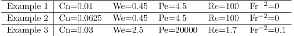
Example 1 Cn=0.01 We=0.45 Pe=4.5 Re=100 Fr−2=0 Example 2 Cn=0.0625 We=0.45 Pe=4.5 Re=100 Fr−2=0 Example 3 Cn=0.03 We=2.5 Pe=20000 Re=1.7 Fr−2=0.1
Table 1: Parameters for the test cases
In the computations, for the spatial discretization, we useP1−P1finite-elements for the phase variables φ and µand P2−P1 Taylor-Hood elements for velocityv and pressure p on uniform meshes with square elements. For time discretization, the stabilizing term is takenβ = 2 and we apply homogeneous Neumann and ho-mogeneous Dirichlet boundary conditions toφ,µandv, respectively, in accordance with (2.37). We also take zero initial velocity v0(x) = 0. The initial conditions for the phase variable,φare determined on the basis of the considered initial fluid volumes.
4.1. Example 1: Coalescence for various density ratios
The goal of this test case is to investigate the time-integration scheme for varying density ratios, ρ2:ρ1. To this end, we consider the coalescence of two sufficiently close but non-touching droplets in a domain Ω = (0,1)2 with time step size ∆t= 0.05 for a matched density case withρ2:ρ1 = 1 : 1 and a very large density-ratio scenario with two heavier droplets set in a lighter ambient medium with ρ2:ρ1 = 1 : 1000. One may note that the latter ratio is very high when compared with other numerical results in the literature. For both cases, we ignore the effect of gravity. The other parameters are listed in Table 1. We set the initial condition for the phase variable according to:
φ0(x) = 1−
2
X
i=1 tanh
p
(x−xi)2+ (y−yi)2−ri
Cn√2
!
(4.1) withr1= 0.25 andr2= 0.1 and (x1, y1) = (0.4,0.5) and (x2, y2) = (0.78,0.5). The initial condition (4.1) represents two circular droplets with radiir1andr2centered at (x1, y1) and (x2, y2). We cover Ω with a spatial mesh composed of 1282 uniform elements, which provides a support structure for the finite element spaces detailed above.
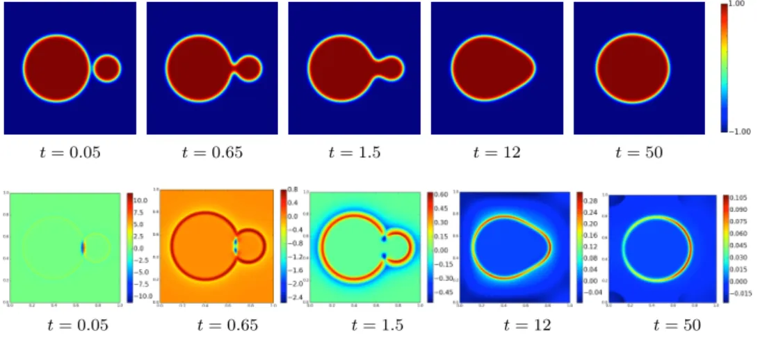
Figure 2 and the top row of Figure 3 present the evolution of the phase variable for the matched and the non-matched density cases, respectively, from t = 0.05 to 50. One can observe that for both the matched and non-matched density cases, the droplets coalesce and form a circular droplet. The initial coalescence can be attributed to diffusion, while the evolution to the stationary circular shape is due to capillary forces which have the effect of minimizing surface area.
t= 0.05 t= 0.65 t= 1.5 t= 12 t= 50
Fig. 2: Droplet coalescence for matched densities: Evolution of phase variable, φ with
density ratio ρ2:ρ1 = 1 : 1, fromt= 0.05 to 50, Cn= 0.01, We=0.45, Pe=4.5, Re=100,
Fr−2= 0 and ∆t= 0.05
t= 0.05 t= 0.65 t= 1.5 t= 12 t= 50
t= 0.05 t= 0.65 t= 1.5 t= 12 t= 50
Fig. 3: Droplet coalescence for non-matched densities: Evolution of phase variable, φ
(top) and divergence of mixture velocity (bottom) with density ratio ρ2:ρ1 = 1 : 1000,
fromt= 0.05 to 50, Cn= 0.01, We=0.45, Pe=4.5, Re=100, Fr−2= 0 and ∆t= 0.05
behavior. It can be observed that the divergence of the mixture velocity is non-zero, i.e.∇ ·v6= 0, in the vicinity of the moving interface, where compressible mixing of the phases occurs. In the pure phases away from the interface, for which the indi-vidual components are incompressible, we indeed observe that the mixture velocity is solenoidal, i.e. ∇ ·v = 0. As opposed to the non-matching density case, for the matching-density case the incompressibility condition is satisfied up to discretiza-tion errors throughout the domain, in the pure phases as well as at the interface (results not displayed).
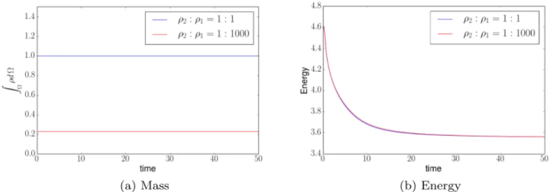
(a) Mass (b) Energy
Fig. 4: Evolution of mass and energy for the droplet-coalescence test case for matched
densitiesρ2:ρ1= 1 : 1 and non-matched densitiesρ2:ρ1= 1 : 1000.
discrete energy-dissipation property of the time-integration scheme according to Theorem 3.2.
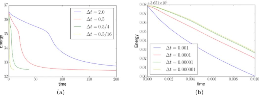
4.2. Example 2: Breakup of two droplets with large time step size
This test case serves to study the stability of the scheme in Algorithm 1 for large time steps. We regard a rectangular domain Ω = (−2,2)×(−4,4). The domain is covered with a mesh composed of 75×150 elements, which again supports finite-element approximation spaces as before. We consider a large density ratioρ2:ρ1= 1 : 1000 and a large time step ∆t= 0.5. The considered setup pertains to breakup of two droplets of identical size connected by a thin liquid bridge. We take the dimensionless parameters as presented in Table 1.
Figure 5 shows snapshots of the evolution of the phase field. One can observe that the liquid bridge that initially connects the two droplets fissures under the effect of surface tension and the separate droplets subsequently evolve to a circular shape in time, during which their surface area decreases.
t= 0.5 t= 10 t= 14 t= 25 t= 55 t= 150
Fig. 5:Breakup of a liquid bridge between two droplets for a large density ratioρ2:ρ1=
1 : 1000 and with large time-step size ∆t= 0.5: Evolution of phase variable fromt= 0.5
to 150 (Cn= 0.0625, We=0.45, Pe=4.5, Re=100, Fr−2= 0).
reported in the literature are of the order of 10−3. By virtue of the fact that our time-integration scheme retains its stability even at such large time-step sizes, it provides a solid basis for time adaptivity. In Figure 6(b) we consider the energy dissipation of the time-integration scheme in the limit ∆t→0. To this end, we plot the evolution of the energy versus time for ∆t={10−6, . . . ,10−3}. One can observe that the energy evolution converges as ∆t→0 and that small but finite dissipation remains in this limit, in accordance with the energy dissipation of the underlying quasi-incompressible NSCH equations. The total mass is preserved independent of the time-step size (results not displayed).
(a) (b)
Fig. 6: Energy evolution for breakup of a liquid bridge between two droplets for density
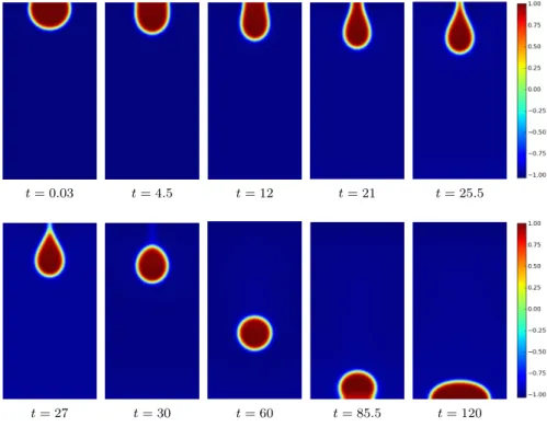
4.3. Example 3: Pinching droplet
In this third test case, we explore the time-integration scheme subject to the effect of gravity. We consider a domain Ω = (−0.3,0.3)×(−0.8,0.8) composed of 60×200 uniform square elements supporting the previously defined finite-element approxi-mation spaces. Note that the computational domain is restricted to the right half of Ω in view of symmetry. The initial condition corresponds to a droplet attached to the top boundary:
φ0(x) =−tanh
p
x2+ (y−2.9)2−0.35
√
2 Cn
!
see Figure 7. The parameters are set in accordance with Table 1. For this example, we set the density ratioρ2:ρ1= 1 : 2.5, because at large density ratios the condition ρn>0 can be violated for the considered large time-step size.
The evolution of the phase-field corresponding to the falling droplet is presented in Figure 7. Initially, the droplet is attached to the upper wall. In time, due to gravity it moves downward and after detaching from the upper wall it continues its
t= 0.03 t= 4.5 t= 12 t= 21 t= 25.5
t= 27 t= 30 t= 60 t= 85.5 t= 120
Fig. 7: Evolution of the phase variable for a pinching droplet subject to gravity with
density ratio ρ2:ρ1 = 1 : 2.5 from t = 0.03 to 120 (Cn= 0.03, We=2.5, Pe=2×10⁴,