Modeling and control of operator functional state in a unified framework of fuzzy inference petri nets

Abstract

Background and objective: In human-machine (HM) hybrid control systems, human operator and machine cooperate to achieve the control objectives. To enhance the overall HM system performance, the discrete manual control task-load by the operator must be dynamically allocated in accordance with continuous-time fluctuation of psychophysiological functional status of the operator, so-called operator functional state (OFS). The behavior of the HM system is hybrid in nature due to the presence of both discrete task-load (control) variable and continuous operator performance variable.

Methods: Petri net is an effective tool for modeling discrete event systems, whereas for hybrid system involving discrete dynamics, generally Petri net model has to be extended. Instead of using different tools to represent continuous and discrete components in a hybrid system, this paper proposed a method of fuzzy inference Petri nets (FIPN) to represent the HM hybrid system comprising a Mamdani-type fuzzy model of OFS and a logical switching controller in a unified framework, in which the task-load level is dynamically reallocated between the operator and machine based on the model-based OFS prediction. Furthermore, for the purpose of validation of the framework suggested, this paper used a multi-model approach to predict the operator performance based on three electroencephalographic (EEG) variables via the Wang-Mendel (WM) fuzzy modeling method. The membership function parameters of fuzzy OFS model for individual experimental participant were optimized by using artificial bee colony (ABC) evolutionary algorithm. Three performance indices, RMSE, MRE, and EPR, were computed to evaluate the overall modeling accuracy.

Results: Experiment data from six participants are processed and simulated, the results show that the proposed method(FIPN with adaptive task allocation) yields better performance with lower breakdown rate(from 14.8% to 3.27%) and higher human performance(from 90.30% to 91.99%).

Conclusions: The simulation results of FIPN-based adaptive HM (AHM) system on six experimental participants demonstrated that the FIPN framework provides an effective way to model and regulate/optimize the OFS in HM hybrid systems composed of

This work was supported in part by the National Natural Science Foundation of China under Grant No. 61075070 and Key Grant No. 11232005.

*_{Corresponding author at: School of Information Science and Engineering,}

East China University of Science and Technology, 130 Meilong Road, Shanghai 200237, P.R. China. Tel: +86 21 64253808

E-mail address: [email protected].

continuous-time model of OFS and discrete-event switching controller.

Keywords: Man-machine system; Fuzzy inference Petri net; Operator functional state; Human performance; Adaptive functional allocation; Electroencephalography

Acronym AA Adaptive Automation ABC Artificial Bee Colony

ANFIS Adaptive-network-based Fuzzy Inference Systems ATA Adaptive Task Allocation/Allocator

AutoCAMS Automation-enhanced Cabin Air Management System DPN Differential Petri Nets

EEG Electroencephalograph FIPN Fuzzy Inference Petri Net

FIS Fuzzy Inference Systems

HM Human-Machine

LAS Level of Actuator Sensitivity

NOS Number of Subsystems requiring manual control ODE Ordinary Differential Equations

OFS Operator Functional State

PN Petri Nets

SA Situational Awareness TIR Time in Range TSK Takagi-Sugeno-Kang

WM-method Wang-Mendel fuzzy modeling method Mathematical symbol K number of fuzzy rules in the rule-base MF Membership Function

i

m Matching degree of the i-th fuzzy rule

k

m marking in place k ,

o_{p p}o _{pre- and post-transitions of place p} ,

o_{t t}o _{pre- and post-places of transition t} ( )

T t Measured TIR at current time instant t ˆ( )

T t Predicted TIR at current time instant t u(t) Control input at current time instant t

( )_j

V T firing speed of differential transition Tj

W incidence matrix

yi _{center of the output MF in the i-th rule}

Fuzzy Modeling and Control of Operator

Functional State in a Unified Framework of

Fuzzy Inference Petri Nets

Jian-Hua Zhang

a,*

_{, Jia-Jun Xia}

a

_{, Jonathan M. Garibaldi}

b

_{, Petros P. Groumpos}

c

_{, and Ru-Bin Wang}

d

a_{School of Information Science and Engineering, East China University of Science and Technology, Shanghai 200237, P.R. China.} b_{School of Computer Science, University of Nottingham, Nottingham, NG8 1BB, UK.}

c_{Department of Electrical and Computer Engineering, University of Patras, 26500 Rion, Patras, Greece.}

him/her to cope with unforeseen emergency or urgent events in real time. Thus, it is necessary to find a way to allocate dynamically the tasks between human operator and machine computer. In this connection, adaptive allocation of task-load is important for a large class of human-machine integrated systems. An adaptive task allocation (ATA) strategy was integrated into a human-machine process control system to assign some of the control tasks to computer-based controllers temporarily once the risky operator functional state (OFS) is detected in [1]. In [2], the following switching logic was proposed: when OFS is effective, the current task allocation remains unchanged; when risky OFS caused by a loss of SA occurs, several tasks would be assigned to operator to keep his/her maximum engagement with the tasks; and when risky OFS caused by high cognitive load is detected, several tasks for operator would be reallocated to computers temporarily with particular aiding (or assistive) strategy triggered. In this way, operator can be attentive but without cognitive overload and the operator performance (including SA) may be maintained at a desired level.

In order to achieve adaptive functional allocation, accurate assessment of OFS is essential. In our previous work [3], support vector machine was used to classify the mental workload, whereas in[4] and [5], the index time in range (TIR) was used to quantify the operator performance and both adaptive-network-based fuzzy inference systems (ANFIS) and genetic algorithm (GA) based fuzzy systems were used to evaluate the OFS. The work demonstrated that fuzzy system is a powerful tool for OFS assessment. In [1] and [6], the authors built predictive models to predict the OFS based on the measured electroencephalographical (EEG) data. The ATA is inspired by model predictive control (MPC) technique. A model based hybrid predictive control was proposed in [7], where the model is fuzzy. The work in [8] showed that for hybrid system with discrete inputs, satisfactory control performance can be attained by employing the MPC with fuzzy models.

Since the relationship between the operator performance and electrophysiological markers is generally unknown, complicated and uncertain, the data-driven models are usually used to characterize the OFS. Subject-specific models were built considering noticeable individual difference. For each subject, we constructed an individualized model based on the

Evolutionary algorithm is usually time-consuming (or computationally intensive). If the parameters in objective function are model-related and the model-construction procedure is complex, the whole evolutionary optimization procedure is even slower. Compared with the time-consuming convergence of evolutionary algorithms with time-consuming modeling methods, WM method provides a promising alternative for OFS model construction.

nets (FTPN) were proposed in [21] and [22]. Ding et al. assigned a fuzzy firing time to the transitions in FTPN [21 whereas in [22] the timing effect was represented by fuzzy sets. Though FTPN performs well in (discrete) process modeling, it is not sufficient to model a continuous-time fuzzy system. Based on DPN, Ding et al. used PNs to represent switched Takagi-Sugeno-Kang (TSK) fuzzy systems [23]. Their work provides a way to analyze the switched fuzzy systems by checking the properties of PN (such as deadlock detection [24]) and to use the PN model for further system implementation. These work showed the strength of PNs for representing fuzzy inference systems (FIS). It is well-known that the TSK and Mandani types are two major classes of FIS. The TSK fuzzy models have been widely used in the aforementioned work in virtue of its ease of mathematical analysis. Nevertheless, TSK fuzzy models might not be suitable for representing the linguistic-rule-based knowledge. Due to the interpretable rule base, Kaur et al. suggested the use of Mamdani-type FIS particularly for decision support applications [25].

Based on DPN [15], in this work we proposed a new type of Petri nets, named fuzzy inference Petri nets (FIPN), to represent the behavior of hybrid system, i.e., the continuous and discrete part of FIPN is fuzzy model (OFS model here) and task allocator (controller here), respectively. In this work, HM system is treated as a hybrid dynamic system; FIPN is the method for modeling HM system. However, with only data, FIPN could not be able to model the system. So the data-driven modeling method-WM method could be employed, and Mamdani-type fuzzy rules could be generated. What’s more, the parameters in WM method should be optimized for a better performance, so Artificial Bee Colony (ABC) was employed to enhance the performance of WM method. For the purpose of validation of the proposed method, we used an individualized fuzzy model to predict the OFS of an operator. On the basis of that, dynamical task reallocation is realized. There is already several existing work on OFS modeling, e.g., [1-6]. Nevertheless, most of the developed models using TIR as the model output are basically not dynamical, but static. However, the current value of TIR may be highly correlated to its historical data. For this reason, in this work we took the difference of TIR between two neighboring sampling instants as the model output. Moreover, we calculated three performance indices, namely root mean square error (RMSE), mean relative error (MRE) and effective prediction rate (EPR), to evaluate different aspects of fuzzy modeling performance.

The remainder of this paper is organized as follows: In Sect. 2, we describe the data acquisition experiment and data preprocessing scheme. Section 3 introduces the ABC-based WM method and proposes fuzzy inference Petri nets. In Sect. 4, fuzzy model of HM system is constructed and simulation of ATA-based HM system is performed to validate the feasibility of the proposed method. Section 5 concludes the paper with an outline of future work.

2. Experiments and Data Preprocessing

To acquire physiological data of human operator under different levels of cognition-demanding task-load, we designed data acquisition experiment using an experimental procedure similar to that in our previous work [26]. A detailed description of the experimental design scheme and procedure is given in this section.

2.1 Experimental Environment

The machine part of HM system is simulated by a software simulation platform, developed by Hockey, Manzey and others [28] to simulate Automation-enhanced Cabin Air Management System (AutoCAMS) on board of a spacecraft, submarine or other safety-critical and self-contained systems, another version of which was also used in [4]. As will be shown later, in comparison with [4] we designed different experimental procedure and used a different number of measurement electrodes in the current study. The AutoCAMS consists of four subsystems: O2 concentration, air pressure, CO2

concentration, and temperature. Each subsystem can be controlled by either human operator in manual mode of operation or by computer in automatic mode of operation. The output trajectories of these four subsystems were monitored and displayed in real time. The level of actuator sensitivity (LAS) is also variable for each subsystem. In the experiment, we used standard and high LAS. Under high LAS, the controlled variable is changing rapidly (i.e. operator must pay more attention on the system functioning and thus mental workload of the operator is high), while standard LAS leads to a more sluggish process. Take O2 subsystem as an example; in

standard LAS it pumps 0.07% O2 into the cabin from oxygen

tank every second when the valve is open, whereas in high LAS the rate is 0.22% per second. With high LAS, the changing rate is much higher and manual control tasks imposed on the operator become more difficult, indicating a higher level of task difficulty than standard LAS, hence an operator has to attentively invest more mental effort in order to manually control the entire system around desired set-points. The EEG data was measured by using Nihon-Kohden equipment connected to the experimental PC. The AutoCAMS software was run on another laptop computer.

2.2 Experimental participants and procedure

three to five days before the first formal experimental session, to make sure that he is capable of skillfully commanding manual control tasks under Auto-CAMS task environment. Through the specifically-designed training procedure, all participants became familiar to the software simulation platform as well as the manual control task skills and the manifest performance decline is usually due to mental fatigue accumulated during the long-duration session and/or low (or poor) OFS, instead of lack of manual skills and/or experience.

Each participant was engaged in two sessions of experiment, which were conducted starting from 2:00 PM on Friday of two different weeks. Each session lasted 50 min, which consists of 10 task-load conditions each lasting 5 min. In conditions 1, 4, 7, and 10, all four subsystems were automatically controlled by the computer and the participant was in a relaxed state. Under conditions 2, 5, and 8, the participant was required to manually control 2, 3, and 4 subsystems, respectively, in the case of standard LAS (as described in Sect. 2.1). More challenging manual control tasks appeared in conditions 3, 6, and 9 (i.e., the number of subsystems to be manually controlled was 2, 3, and 4, respectively) in the case of high LAS. At the end of each task-load condition (with different NOS or LAS in experiment), the participant was asked to subjectively report their estimated (or perceived) level of mental fatigue, mental effort and anxiety on a rating scale of 0 - 100 points (see also our previous work [26]). The task-load conditions in a session of experiment are illustrated in Fig. 1. The task of participants is to control specific subsystems according to the process control requirement in each condition.

2.3 Data preprocessing

Using the measurement electrode placement scheme shown in Fig. 2, we recorded the EEG data. The placement of electrodes was based on 10-20 international electrode system. Since ocular artifacts may seriously contaminate the EEG signal, we also recorded the vertical electrooculogram (VEOG) from two electrodes placed above and below the left eye of the participant (those electrodes might be removed in our future experiment with the method proposed in [27]). Ocular artifacts were removed by using the same independent component analysis (ICA) technique as that in [1]. In this way, clean EEG data was acquired.

The raw EEG data was sampled at 500 Hz. Since the maximum frequency of EEG signal is usually lower than 40 Hz, the power spectrum density (PSD) of EEG signal was computed via fast Fourier transform (FFT) on a 5-sec segment of EEG data. Each EEG measurement channel involves 10 features (each covering a 4 Hz bandwidth, as shown in Table 1).

The operator performance (quantified by time in range - TIR) was calculated every second by:

(1)

(%)

'

100

T

n

n

= ×

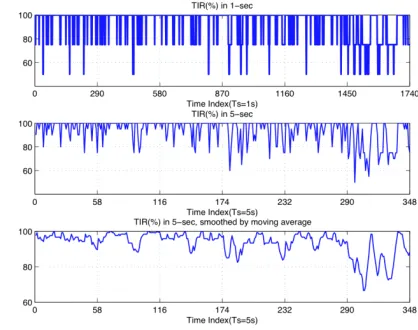
where n′ and n denote the number of subsystems in target ranges and the number of subsystems, respectively. Subsequently the original TIR data was evenly segmented into 5-s segments, each of which was averaged to make the size of EEG and TIR data identical. Take participant C, Session 1 as an example, as shown in Fig. 3. The original TIR data was shown in the top sub-figure of Fig, 3, where TIR takes the five discrete values of 0, 1/4, 2/4, 3/4, or 1 every second (i.e., the temporal resolution is 1 s). The result of the 5-sec segment averaging is presented in the middle sub-figure of Fig. 3, where TIR∈(0,

[image:4.595.347.501.124.259.2]

Fig. 2: EEG electrodes placement, including 17 electrodes with two referential electrodes (i.e., A1 and A2) placed on earlobes.

[image:4.595.69.276.126.234.2] [image:4.595.330.539.299.464.2]

1/20, 2/20, …, 1) takes 21 or less discrete values every 5 s (i.e., the time resolution becomes 5 s). However, intuitively the temporal fluctuation of OFS should be smoother than the change of TIR shown therein. Thus, we smoothed the resulting TIR data by moving average with a sliding window length of 30 s and step size of 5 s. Finally the preprocessed TIR data, used as the model output data later, is depicted in the bottom of Fig. 3.

In high LAS condition, the system is varying rapidly and thus the participants have to be trained for a long time to execute the manual control tasks skillfully and successfully. For this reason, the performance breakdown in high LAS might correspond to either poor OFS or other factors such as long reaction time. The data elicited from high LAS is very noisy and hard to interpret. So here we only consider the case of standard LAS, i.e., only the EEG data in conditions 3, 6, and 9 were taken into account. In condition 10, the participant was relaxed without any manual control demand. Furthermore, as mentioned above, participants were asked to rate their perceived level of mental fatigue, mental effort and anxiety during that time, however the step of subjective ratings and task-load level switching would possibly interfere in the EEG data recording. The removal of the 5-sec data segment was based on participants’ experience, which is long enough to eliminate the unwanted interference from the measured data. Thus, there were 58 data points in each condition and 348(=58*6) data points for each measurement channel. Finally, the data of each feature set was normalized to the unit interval [0, 1].

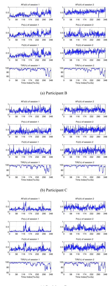
In this work, we selected AF_z,θ,P_z,αand F_z,θ as the input features of OFS model; we performed gray relation analysis of the EEG channels and found the most highly related channel

based on the time-series data of 6 participants data. The ,

z AFθ

other two channels were chosen based on previous work. For the reasons for selecting the specific EEG channels, the interested readers are referred to Ref. [1] and [2]. The three model inputs (i.e., EEG spectral power features) and single output (i.e., the primary-task performance variable of the operator, TIR) for participant B, C, and D are presented in Fig. 4.

3 Methods

3.1 ABC-based Wang-Mendel fuzzy modeling method

The ABC algorithm is a swarm optimization based meta-heuristic algorithm. It was inspired by intelligent foraging

(a) Participant B

(b) Participant C

[image:5.595.76.240.118.255.2]

(c) Participant D

Fig. 4: The I/O discrete-time data (EEG averaged every 5 s, TIR smoothed by moving average of 5s) from two sessions.

Table 1

The Features from the EEG Fz channel

Index Feature

1 Fz,δ(1-4Hz)

2 Fz,θ(5-8Hz)

3 Fz,α(9-12Hz)

4 Fz,β1 (13-16Hz)

5 Fz,β2 (17-20Hz)

6 Fz,β3 (21-24Hz)

7 Fz,β4 (25-28Hz)

8 Fz,β5 (29-32Hz)

9 Fz,γ1 (33-36Hz)

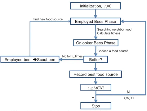
[image:5.595.324.533.120.669.2]

behavior of honey bees. In fact, GA, PSO and ABC algorithms were compared in our work. It turned out that the newer ABC algorithm leads to relatively better optimization result, details could be found in Sect. 4.2. In ABC algorithm, the colony of artificial bees contains three groups of bees: employed bees associated with specific food sources, onlooker bees watching the dance of employed bees within the hive to choose a food source, and scout bees searching for food sources randomly. Fig. 5 is a flowchart of ABC algorithm used to tune the parameters of fuzzy OFS model, in which tc is the cycle number, MCN is the maximum number of cycles, and tac is a predetermined “abandonment criterion”. A detailed description of the ABC algorithm can be found in [29].

The WM method is an efficient way to learn fuzzy rules from numerical data. For MISO system, its procedure basically consists of the following five computational steps:

Step 1 (Partition I/O domains into fuzzy subsets): Partition

each dimension of I/O domains into 2N+1 fuzzy regions and each region is assigned with a membership function (MF) with a linguistic label. In our work we chose Gaussian MFs, reasons provided in the end of this sub-section. The MF parameters were optimized by using artificial bee colony (ABC) algorithm.

Step 2 (Generate fuzzy rules from given data pairs): For a given I/O data pair, the membership degree of each dimension in different regions is determined. For each dimension, the linguistic label with the maximum membership degree is regarded as its label. The antecedent of a fuzzy rule is generated by connecting all inputs’ linguistic labels with logical “AND", while its consequent is the output’s linguistic label. The fuzzy rule generated in this step is in the following form:

IF x1 is A1 and x2 is A2 and … and xn is An, THEN y is B.

Step 3 (Assign a degree to each fuzzy rule): Due to the possibly large size of sample dataset, probably there would be some redundant or conflicting rules (i.e. rules with same antecedent part but different consequence part). To cope with this possibility, one way is to assign a (confidence) degree to each rule, and accept only the rule with maximum degree in the conflicting group. A commonly-used method to assign the

degree of the rule is to multiply all the membership degrees of its antecedents.

Step 4 (Create a combined fuzzy rule-base): Some a priori information and expert experience can be incorporated to create a combined fuzzy rule base.

Step 5 (Defuzzification): This step uses the centroid defuzzification method given by:

(2) 1

1 K i i i

K _i i

m y

m

y

=

=

⋅

=

∑

∑

where _yi denotes the center of the i-th output region, _mi is the degree of the i-th rule (usually the product of the input membership degrees), and K is the number of fuzzy rules.

Note that, according to the original Wang-Mendel method [9], the I/O space is partitioned to fuzzy sub-regions and the fuzzy rules are generated from individual training (sample) data pairs (see Steps 1 and 2). However, there may be no training data in some fuzzy sub-regions, but some testing data might fall into those regions. For those regions, there would be no fuzzy rules generated due to the lack of training data. In this condition, other types (such as triangular or trapezoid) of MFs would lead to zero degree of confidence (mi _{in Eqn. (2)) for fuzzy rules}

generated in other regions (the input membership degree might be zero). With Gaussian MFs with an infinitely wide support, although the confidence degree may be very small, there is still an output of the model. There are also other methods for tackling this issue. For example, in [33] the generated rules were extrapolated to the entire space. Nevertheless, the use of Gaussian MFs is the most straightforward one.

For example, if the input space of a system is partitioned as in Fig. 6, there would be no training data (black dots) in the regions 1, 3, 5, 7, and 9. As a result, no fuzzy rules would be generated for those regions. With trapezoid MFs (solid line), if a testing data (red star) falls within any of those regions, the degree of membership to regions 2, 4, 6, 8 are 0, hence each mi

= 0 in Eqn. (2) and no output would result. However, with Gaussian MFs (dashed line), the degree of membership of the testing data to fuzzy rules generated from regions 2 and 4 would be non-zero and thus some output would be acquired from the fuzzy rules generated.

[image:6.595.52.289.113.293.2]

On the other hand, the Gaussian MF is differentiable to an

[image:6.595.355.514.115.255.2]

Fig. 5: Flowchart of the ABC-based optimization algorithm.

infinite degree, it is suitable to be used in any gradient-based optimization algorithm (such as the commonly-used steepest gradient descent technique). In [35], Wang and Mendel proved mathematically that with a sufficient number of fuzzy partitions and fuzzy rules, a fuzzy system, whose output can be expressed explicitly as a linear combination of fuzzy (Gaussian) basis functions, is capable of approximating any real-valued continuous function on a compact set to arbitrarily high accuracy. Hence, we adopted Gaussian MFs in this work. A detailed introduction of WM method could be found in [9] and [33].

3.2 Fuzzy inference Petri net

In this section, a new fuzzy inference Petri net method is proposed based on differential Petri net (DPN). The DPNs were usually used to model hybrid systems in which continuous part was described by differential equations [15], but in our work Petri nets were used to model fuzzy rule-based systems with no need of precisely-known first principles.

As pointed out above, fuzzy inference Petri net (FIPN) is an extension of DPN, which is defined as DPN=<P, T, Pre, Post, f, M0, J>, where P is a finite set of places; T is a finite set of transitions; Pre( , )P Ti j is a function that defines arcs from a place to a transition; Post( , )P T_{i j} is a function that defines arcs from a transition to a place; f P T: ∪ →

{

D DF,

}

indicates two types of place and transition, D for discrete type and DF for differential type; M0 is initial markings, and J is a “timing map” which associates a time (real number) with every transition.

The following notation will be used: o_pand _po are the pre- and post-transitions of place p; and are the pre- and post-o

t o

t

places of transition t; and W is an incidence matrix defined by: (3)

(

)

(

)

[ ]

Post , Pre ,

P T

ij n n

ij i j i j

W w

w P T P T

× = ⎧⎪ ⎨ = − ⎪⎩

For the timing map J, the following two relations hold: If f ( ) = D, thenTj J( )Tj =dj (i.e., a delay is associated with the discrete transitionTj); and

If f ( ) = DF ,thenTj J( )Tj = V T h( )j , where the maximum firing speed V T( )_j can be either a constant or a function of the markings of the differential places connected to the differential transition and h is the time constant.Tj

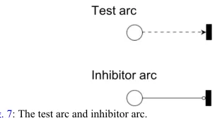
In FIPN used for the purpose of system modeling, two new types of arc are introduced in addition to all the components in

DPN: One is “test arc” and another is “inhibitor arc”, as shown in Fig. 7. Test arc is similar to normal arc in its role in enabling transitions, which is like an arc from a place to transition and a reciprocal arc with the same weight but does not consume any tokens (or continuous marking) upon firing of the transition (as a result, conflicts can be reduced). Inhibitory arc was first introduced by Agerwala [30] and widely used in performance modeling and simulation analysis[31]. It prevents a transition from firing if the marking of input place at least equals the weight of the arc and this behavior does not consume any tokens.

A FIPN for switched fuzzy systems basically consists of three parts, namely fuzzy inference (continuous) part, step control (discrete) part, and switching logic part (discrete too).

Definition 1: A marked graph is a Petri net in which each place has exactly one input and one output transition [32], i.e.,

, for all (4) 1

o o

p = p = p P∈

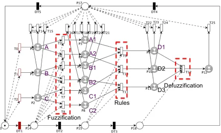
According to Definition 1, we can use a marked graph as the step control part of FIPN. As an example of FIPN modeling, we use a 3-input single output fuzzy model with the following three fuzzy rules:

R1_{: IF A is A}

1 and B is B1, THEN D is D1. R2_{: IF A is A}

2 and C is C1, THEN D is D2. R3_{: IF B is B}

2 and C is C2, THEN D is D3.

The Petri net representation of the above fuzzy model is shown in Fig. 8. The fundamental idea of FIPN is that DPN is equivalent to an FIS if appropriate speed functions are set for it. The marked graph can enable or disable the differential transitions. A token in place P13 can enable the input transitions (with test arc), and after firing P14 takes a token away from P13. This disables the input transitions but enables the “fuzzification” transitions. Suppose that the holding time for P14 is t0, and the “timing map J” of fuzzification transitions is

, where mf is the membership function. After the firing 0 0

mf t t

of the fuzzification transitions, the post places would acquire tokens.

0 0 mf

t × =t mf

When there is a token from P14 to P15, the “rules” transitions are enabled. The J of rule transitions is

₀ (5) 0

o k k tm _t

t

∈

∏

where

∏

_k∈o_tmk is the product of markings in all preplaces of transition t. The next event after “rules” is centroid defuzzification (Step 5 in Sect. 3.1). The mi _{in Eqn. (2) are} calculated by the previous “rules” transitions and are exactly the markings in places D1, D2, and D3. When the weights of the arcs are set as the centroid iand J of the transitions is

y

(6) 1

0 0

( o ) ( o )

i

k k

k tm k tm y _t t

−

∈ ∈ ⋅

∑

∑

[image:7.595.62.214.115.199.2]

The “defuzzification” transition will automatically perform the defuzzification step. Place P17 controls the “initialization” step since it can enable all the differential transitions (so-called “sink transitions”) on the top of Fig. 8. The firing speed of these transitions equals the markings in o_tdivided by the time constant, hence after firing the state of FIPN will be re-initialized and new input data can be processed without the influence of historical data.

The evolution graph of this FIPN is shown in Fig. 9, where xi

denotes the model input, µij is the membership degree of xi in fuzzy region j, Mi is the confidence level of output yi calculated by the “rules” transitions, ( K₁ i) ( K₁ ) is the

i i

i i

y=

∑

₌m y⋅

∑

₌m

model output, and “...” represents complicated but meaningless markings. After all the calculation, the “initialization” step resets the FIPN for the presentation of the next input.

4 Control and Simulation of Human-Machine Hybrid System

The modeling, control and simulation of a switched fuzzy system are considered in this section. We generated a fuzzy predictive model for the HM system and then mapped it to fuzzy inference part of an FIPN. Afterwards we proposed a switching logic for the FIPN to realize ATA. The block diagram of HM control system is shown in Fig. 10.For each

Fig. 8: A schematic configuration of FIPN representing a fuzzy model comprising three fuzzy rules.

[image:8.595.87.539.108.382.2] [image:8.595.95.237.512.735.2] [image:8.595.313.548.593.740.2]

participant, the data measured from the 1st _{experimental session}

were used to construct the model while the data from the 2nd

session were used as the testing set to check the generalizability performance of the model developed.

4.1 Predictive OFS model

The improved WM method was proposed in [33]. Here we use a one-step-ahead predictive model:

(7)

ˆ( 1) ( ) [ ( )]

y t+ =y t +Fut

where u

( )

t denotes the EEG input vector, y tˆ( 1)+ denotes for model output (i.e., TIR time-series) and y(t) is the real TIR value at time step t,. respectively.

Eqn. (7) can be rewritten into:

∆y tˆ

( )

= ⎡F_⎣u

( )

t ⎤_⎦ (8) where ∆y tˆ

( )

=y tˆ

(

+ −1

) ( )

y t .

The fuzzy model predicts the temporal change of TIR, namely ∆TIR, instead of TIR itself. This is more reasonable since TIR is a time-dependent performance variable whose current value is dependent upon its past values.

As mentioned in Sect. 2.3, three inputs (AFz,θ,Pz,αand Fz,θ) are empirically selected. Since each input fuzzy subset requires a place in FIPN, in order to reduce the dimensionality of incidence matrix W, all three input domains are partitioned into

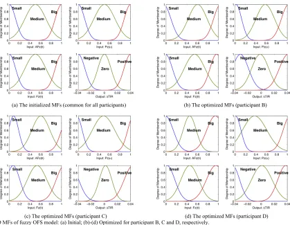
3 fuzzy subsets with linguistic labels of Big, Medium, and Small and the output domain is partitioned into 3 fuzzy subsets with linguistic values of Negative, Zero, and Positive. Fig. 11 shows a comparison of fuzzy division of I/O domains before and after optimization. The MF parameters were optimized by the ABC algorithm. We quasi-equally divide the data measured from 1st

experimental session into 5 parts, i.e. 5-fold cross-validation. During the process of model construction, we used four fifth of the 1st _{session data as the training set to train a model and the}

rest of the one fifth data as the validation set to further tune the model parameters, and the model parameters are average values of the results of 5-time optimizations. In every time of optimization, the training set was used to train a model with WM method and initial parameters, and validation set was used to calculate RMSE. In this way, the over-fitting problem is mitigated.

For the ABC-based optimization algorithm, colony size was 40 (including 20 employed bees and 20 onlooker bees), MCN=1000, and tac=100. The initial food source xm is calculated by:

(9)

(0,1) ( )

mi i i i

x = +l rand × u −l

where xmi is the i-th component of xm, ui and are the lower li and upper bound of xmi, respectively. The objective function of ABC is RMSE in Eq. 10:

(a) The initialized MFs (common for all participants) (b) The optimized MFs (participant B)

[image:9.595.87.506.127.452.2]

(c) The optimized MFs (participant C) (d) The optimized MFs (participant D)

(10)

(

)

2

1 1

1 1 ( 1) ˆ( 1)

N

N k

RMSE= ₋

∑

₌− y k+ −y k+

where y t( ) and y tˆ( ) are the actual and model output at time step t, respectively and N is the size of testing dataset. Note that, the model is a predictive model, which means the model output is a prediction of TIR in next time step. So there will be only N-1 point-pairs to calculate.

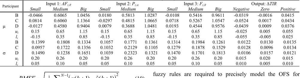
For each fuzzy OFS model, xm is the parameter vector of the I/O Gaussian MFs, each containing central (or mean) parameter

µ and width (or standard deviation) parameterσ, given by: (11) 1 1 1 1 1 1 2 2 2 2 2 2 3

3 3 3 3 3 [

] m s s m m b b s s m m b b s

s m m b b on on oz oz op op

x µ σ µ σ µ σ µ σ µ σ µ σ µ

σ µ σ µ σ µ σ µ σ µ σ =

where s, m and b represent fuzzy subsets small, medium, and big defined in each input domain, respectively; 1, 2, 3, and o represent three model inputsAFz,θ,Pz,α,Fz,θ and model output

∆TIR, respectively; and n, z and p represent fuzzy subsets negative, zero and positive defined in output domain, respectively.

The bounds of the I/O membership function (MF) parameters of all I/O variables in the ABC-based optimization were empirically obtained. Intuitively, the three MF center parameters can be set at 0, 0.5 and 1, respectively. It was also found that fuzzy modeling accuracy is insensitive to the change of upper and lower bounds. In other words, fuzzy models were found to be robust w.r.t. the parameter variation. The model parameter optimization results for participant B, C, D are presented in Table 2 (averaged results from 5-fold cross validation).

Fuzzy rule-bases for participant B, C, and D are shown in Tables 3, 4, and 5, respectively. For different participants, different model (sometimes even different feature [34]) could be applied since individual differences always exist. It is noted that when grid partition method is used, there should be a total of 27 (=33_{) fuzzy rules in a complete rule-base. However, WM}

method generates rules directly from training dataset. As a result, no rules are generated in those regions in I/O space, in which no training data falls. So the number of fuzzy rules by WM method can be highly reduced. In this way, the notorious issue of ‘curse of dimensionality’ can be overcome, i.e., the exponential increase of the number of rules with the input dimensionality is avoided.

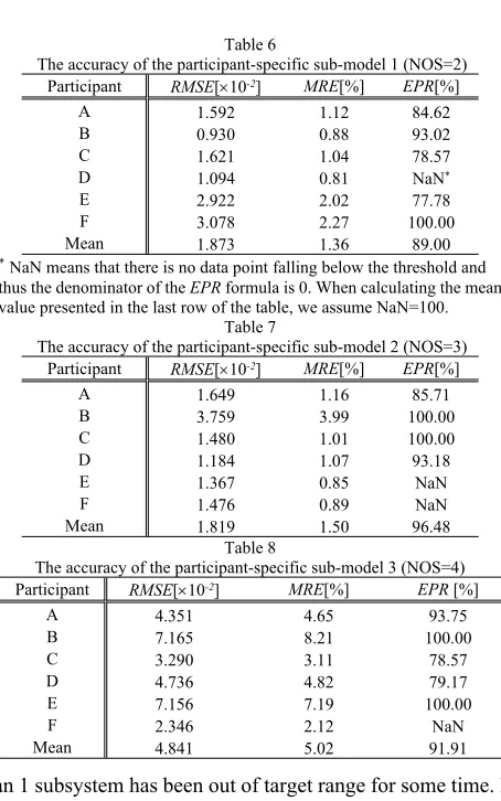
From Tables 3, 4, and 5, it can be seen that only 8, 13, and 12

[image:10.595.49.550.134.264.2]

fuzzy rules are required to precisely model the OFS for participant B, C, and D, respectively. Due to the positivity of Gaussian MF, there always exists a non-zero membership degree for each rule. In other words, all rules in a rule base are fired to certain extent. Even if the testing data is settled out of the training input regions, an accurate output can be calculated owing to the good generalizability of the FIS, who is essentially

Table 3

Fuzzy rule-base of fuzzy OFS model (participant B, NOS=4)

Rule # AFz Pz Fz ∆TIR

1 Small Small Small Zero

2 Small Small Medium Negative

3 Small Medium Small Zero

4 Small Medium Medium Zero

5 Medium Small Small Zero

6 Medium Small Medium Positive

7 Medium Medium Small Zero

8 Medium Medium Medium Positive

Table 4

Fuzzy rule-base of fuzzy OFS model (participant C, NOS=4)

Rule # AFz Pz Fz ∆TIR

1 Small Small Small Zero

2 Small Small Medium Negative

3 Small Medium Small Zero

4 Small Medium Medium Zero

5 Medium Small Small Positive

6 Medium Small Medium Negative

7 Medium Small Big Zero

8 Medium Medium Small Positive

9 Medium Medium Medium Positive

10 Medium Big Small Positive

11 Medium Big Medium Zero

12 Big Small Medium Negative

13 Big Medium Medium Positive

Table 5

Fuzzy rule base of fuzzy OFS model (participant D, NOS=4)

Rule # AFz Pz Fz ∆TIR

1 Small Small Small Zero

2 Small Small Medium Negative

3 Small Medium Small Negative

4 Medium Small Small Zero

5 Medium Small Medium Positive

6 Medium Medium Medium Positive

7 Medium Medium Big Negative

8 Medium Big Medium Negative

9 Big Small Medium Zero

10 Big Medium Medium Zero

11 Big Big Medium Negative

[image:10.595.307.543.351.754.2]

5th rule (i.e., i=5, K=8), µ1,5= 0.6065, σ1,5= 0.1808, µ2,5=0.0180,σ2,5 = 0.1057, µ3,5 = -0.0108, σ3,5 = 0.1314, and µoz

=-0.0016, σ3,5= 0.0130. Given all parameters, we can calculate

the model output for every input by using Eqn. (12), the explicit mathematical formulation of fuzzy model.

As shown in Fig. 10, we used a multi-model approach, i.e., we built sub-models in different task-load conditions. In essence, this approach resulted in a composite fuzzy model which is switched by the level of task-load.

4.2 OFS modeling results

The modeling result RMSE was based on the testing set. To evaluate the overall modeling performance, we calculated three performance indices of MRE, RMSE, and EPR. The first index is computed by:

(13)

1 1

1 1

ˆ

(

1)

(

1)

(

1)

N k

MRE N

y k

y k

y k

− = =

−

+ −

+

+

∑

where y t( ) and y tˆ( ) are the actual and model output at time step t, respectively and N is the size of testing set.

The TIR slightly lower than a preset threshold may indicate that the operator is in a vulnerable or risky functional state. Otherwise, the TIR considerably lower than the threshold may simply indicate operator performance breakdown. The third performance index EPR is thus defined as the rate (in percentage) of correct prediction of those risky, vulnerable or performance breakdown states by the OFS predictive model.

When TIR is lower than certain threshold (preset empirically), the operator is unable to cope with high-workload conditions and task reallocation is required. Hence, the EPR index is an important measure of the ATA system. A model with small RMSE and MRE but low EPR would lead to an ATA system that cannot reallocate the task-load on time. This means that EPR is complimentary to the first two commonly used performance metrics, particularly when the model is used for ATA system design.

We determined the threshold in the following way. We compared the subjective ratings and TIR data and found that in the “subjectively perceived challenging” task-load condition (e.g., NOS=4) the TIR values are usually lower than 80%. Furthermore, as the current TIR is influenced by its past values, the TIR is calculated by moving average of its instantaneous values. Thus, when TIR is lower than 80% with NOS=4, more

than 1 subsystem has been out of target range for some time. In the case of NOS=3 or 2, the data points dropped below 80% were rare. Notwithstanding, after a long concentration on the execution of manual control tasks, it is very likely that operator has already been in a vulnerable or high-risk functional state. In the raw data there exist data points where TIRs dropped below 90%, so we preset the threshold for NOS=3 as 90%, while NOS=2 as 95%.

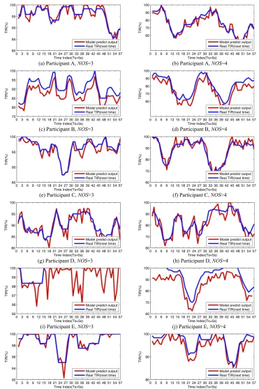
As examples, the sub-model testing results for participant A, B, C, D, E and F are shown in Fig. 12. Note that, the output of the predictive model is a prediction of TIR at the next time step. That is why in Sect. 2.3 we got 58 data points in each condition, whereas in Fig. 12 there are only 57 in each subfigure. In addition, the 1st _{predicted model output should be compared}

with the 2nd _{true TIR. Hence there exists a shift between the true}

TIR and predicted one. In this paper, the indices are made consistent (unified) for an easier comparison.

Table 7

The accuracy of the participant-specific sub-model 2 (NOS=3) Participant RMSE[×10-2_{] MRE[%] EPR[%]}

A 1.649 1.16 85.71

B 3.759 3.99 100.00

C 1.480 1.01 100.00

D 1.184 1.07 93.18

E 1.367 0.85 NaN

F 1.476 0.89 NaN

[image:12.595.315.542.101.464.2]

Mean 1.819 1.50 96.48

Table 8

The accuracy of the participant-specific sub-model 3 (NOS=4)

Participant RMSE[×10-2_{] MRE[%] EPR [%]}

A 4.351 4.65 93.75

B 7.165 8.21 100.00

C 3.290 3.11 78.57

D 4.736 4.82 79.17

E 7.156 7.19 100.00

F 2.346 2.12 NaN

Tables 6, 7, and 8 present the performance indices of the three sub-models in the condition of NOS=2, 3 and 4, respectively. With the increase of NOS, both the modeling RMSE and MRE increase for each participant. This is

reasonable since more dynamical variations in TIR over time are expected with the increase of NOS. In Fig, 11, it can be seen that when NOS=4 TIR takes values in the interval between 60% and 100%, whereas the range shrinks to 80% and 100% when

(a) Participant A, NOS=3 (b) Participant A, NOS=4

(c) Participant B, NOS=3 (d) Participant B, NOS=4

(e) Participant C, NOS=3 (f) Participant C, NOS=4

(g) Participant D, NOS=3 (h) Participant D, NOS=4

(i) Participant E, NOS=3 (j) Participant E, NOS=4

[image:13.595.107.478.116.674.2]

(k) Participant F, NOS=3 (l) Participant F, NOS=4

[image:13.595.109.286.116.678.2]

definition, the lower RMSE and MRE and the higher EPR, the better performance the model possesses. In [1], the three performance indices, RMSE, MRE, and EPR, of the composite model, comprising three sub-models corresponding task-load conditions (NOS=1, 3, and 4) were 9.419*10-2_{, 7.020%, and}

58.9%, respectively. In comparison, the prediction performance indices of our models (NOS=2, 3, and 4) using the difference in TIR as fuzzy model output were improved to 2.844*10-2_{, 2.62%,}

and 92.47%, respectively.

As mentioned before in Sect. 3.1, we also tried the other 2 popular evolutionary optimization algorithms (PSO, and GA) to reveal their respective pros and cons. Set the cross-over and mutation probability as 0.6 and 0.1 respectively, population size as 40, 20 random runs of simulation for each participant and 1000 iteration steps per run, the simulation results of the 5-fold cross validation of the model based on GA are listed in Table 10; whereas the results of PSO algorithm are listed in Table 11 (20 random runs of the simulation for each participant and 1000 iteration steps per run, swarm size 40, learning rate c1=c2=2, inertia weight 0.9).

Comparing the results given in Tables 9, 10, and 11, we can see that most average indices of the GA and PSO are inferior to those of the ABC algorithm. The coding and decoding schemes of GA are complicated. For example, if the binary coding is adopted, an accuracy level of 0.001 for a parameter of the model requires 10 bits. The number of parameters to be optimized is 72, thus for the binary-coded GA, a coded individual/chromosome is rather long (720=72 (# parameters) *10 (length of binary code)). In addition, GA is computationally slow in convergence to the global optima. If choosing different initial populations, the optimization solution found within a limited number of iterations (i.e., 1000) might not be precise enough due to the low probability of mutation operator. Furthermore, as the PSO algorithm is sensitive to the setting of the initial particles in the swarm and sometimes may converge to local optima in a limited number of iterations, the s.d. (standard deviation) of its results is larger. With the existence of scout bees, local optima can be overcome by the ABC algorithm. For the purpose of comparison, the s.d. of ABC algorithm is also calculated. It’s always less than 10-7_,

indicating that the ABC algorithm converges within 1000 iterations. That is why we used the ABC algorithm as the model optimization technique.

Based on the multiple sub-models constructed using the WM method, the control design and simulation of adaptive human-machine (AHM) system are described in the following section. 4.3 Control design and simulation of FIPN-based AHM system

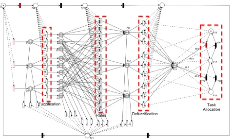
Take the example of participant C, Fig. 13, produced with Hybrid Petri Net ICSI Simulator (HISim) by Alberto Amengual, International Computer Science Institute, illustrates the FIPN used in our control system design (see Fig. 10) and simulation studies. For a different participant, only the “Rules” part varies in Fig. 13. Analogous to Fig. 8, the fuzzy inference part is surrounded by a marked graph, which serves as a step controller with discrete control action. A unique feature of Fig. 13 is that it is essentially a switched (or hybrid) system. The rest parts of FIPN in Fig. 13 are similar to those in Fig. 8, as described in Sect. 3.2. Such a modular simulation system is composed of the following 3 modules:

Module1 - Input data generator: In Fig. 10, the HM system part was simulated based on the measured data. The measured database of the EEG and TIR were available and the NOS switching signal determines which database should be invoked and which data-driven sub-models used. In simulation, first we picked randomly the physiological and TIR data, denoted by and respectively, from the database

( )

k

u n T nk

( )

corresponding to NOS=k, i.e.

uˆ 1

( )

=u nk

( )

(14) Tˆ

( )

1 =T nˆk

( )

(15)

A 6.528±1.756 7.18±2.12 60.07±12.28

B 6.345±2.641 6.91±3.48 71.42±15.06

C 4.272±2.541 4.37±2.99 67.14±22.92

D 5.934±4.028 6.24±4.85 58.93±32.84

E 6.291±4.253 6.20±4.45 95.19±4.97

F 7.153±5.917 7.15±6.15 100±0

Mean 6.087 6.34 75.46

Table 11

The 5-fold cross validation results of the PSO-optimized model Participant RMSE[×10-2] MRE[%] EPR[%]

A 4.148±1.695 4.23±1.91 73.21±14.96

B 4.932±1.128 4.94±1.37 79.83±17.06

C 4.048±1.700 3.96±1.87 68.57±16.44

D 4.768±2.813 4.81±3.40 78.86±9.40

E 4.529±2.392 4.45±2.62 92.78±3.89

F 3.497±2.539 3.34±2.68 100±0

and prior to task-load switching,

(16)

( )

(

)

* ₁

k u t =u t n+ −

(17)

( )

(

)

ˆ ₁

k T t =T t n+ −

where _{u t}*

( )

and _{T t}ˆ

( )

are input data and actual output data at the simulation time step t, respectively. When the NOS switches to s at time instant , we havets

(18) ˆ

arg min ( ) ( )

s

t _{i M} s s

n T t T i σ

∈

= − +

and

, (19)

(

)

( )

* ₁

s s t

u t + =u n

T tˆ

(

s+ =1

)

T ns

( )

t (20) where Ms is the size of database when NOS=s and σ is a random error uniformly distributed in interval [-0.1, 0.1].

Analogous to Eqn. (16) and (17), the following relations hold:

, (21)

(

)

(

)

* ₁

s k t

u t + =t u n + −t

(22)

(

)

(

)

ˆ ₁

s k t

T t + =t T n + −t

Using Eqn. (14) to Eqn. (22), we generated the input and reference output data for the entire simulation.

Module2 - “Rules” transition: In order to simplify the PN structure simpler and reduce the dimensionality of incidence matrix W, the same I/O fuzzy partition but different defuzzification parameters were adopted for the three sub-models with NOS=2, 3, and 4. Since the main task is to prevent operator performance breakdown, we will focus on those time

instants when the OFS is vulnerable or risky, indicated by considerably lower TIR in high-workload conditions. As a result, when generating the fuzzy rule-base, we assigned a higher confidence level to rules generated from those high-risk OFS data. The extracted linguistically-interpretable and transparent fuzzy rule-bases in fuzzy OFS models are explicitly listed in Tables 3, 4, and 5, for participants B, C, and D, respectively.

[image:15.595.60.534.113.399.2]

Module3 - Adaptive task allocator: There are three workload conditions for the operator, in each of which certain number of subsystems demanding manual control (i.e., NOS=2, 3, and 4, respectively). Experiment data suggested that when manually controlling 2 subsystems, operator was in a more relaxed state while performing well the control tasks. This means that in task-load condition of NOS=2 when the mental (or psychological) load is lower, a satisfactory performance (characterized quantitatively by the TIR time-series data) can be maintained by the operator. When NOS=4, a sustained concentration and attention from the operator is demanded and thus after a certain period of time, TIR may decline. The condition when NOS=3 is in between the above two conditions. Once the switching signal NOS changes from 4 to 3, it would be easier for operator to maintain TIR above the preset performance threshold, but the cost is that the mental workload imposed on the operator may be still high. Based on the abovementioned knowledge, the ATA-based control strategy can be designed. The core idea of the ATA strategy is based on the following three intuitively straightforward logical rules:

R1: IF TIR is lower than a threshold (i.e. 80%) and NOS is larger than 2, THEN NOS is reduced; ELSE

R2: IF TIR is higher than a threshold (i.e. 90%) and NOS is less than 4, THEN NOS is increased; ELSE

R3: NOS is held constantly at the current level.

In Fig. 13, the rightmost module functions as ATA. Places P16, P17, and P18 correspond to NOS=4, 3, and 2, respectively. The token in these places enables “defuzzification” transitions with different parameters. The amount of continuous marking in place P15 is TIR (in percentage) and the task-load switching is

achieved by the inhibitor and test arcs (introduced in Sect. 3.2). When TIR is higher than the lower threshold 80%, the inhibitor arcs from P15 to T67 and T78 would disable the transitions. Otherwise the transitions would be normally enabled; token would be taken from the pre-discrete-place of T67 or T78 to their post-places, and thus the control signal NOS would be switched to a lower level. In a similar way, when TIR is lower than the upper threshold 90%, transitions T76 and T87 would be disabled. Otherwise the test arcs from P15 to T76 and T87 would enable the transitions, if the token is not in P16 then, the NOS would be

(a) The performance comparison of the HM system with and without ATA (b) The control signal derived by ATA (participant B) (participant B)

(c) The performance comparison of the HM system with and without ATA (d) The control signal derived by ATA (participant C) (participant C)

[image:16.595.53.524.113.559.2]

(e) The performance comparison of the HM system with and without ATA (f) The control signal derived by ATA (participant D) (participant D)

increased by firing T76 or T87. In this way, the control objective of ATA can be fulfilled.

4.4 Simulation results

All simulation codes were written using Matlab® R2010a and run on a PC with Intel® CoreTM 2 Duo CPU 2.4GHz, 4G RAM and Mac OS X 10.6.8 operation system. Each ATA-based control system simulation was repetitively run 100 times to perform statistical analysis of the results.

Figs. 14(a), 14 (c), and 14 (e) compare the measured operator performance without active control (dotted line in red, NOS=3 and 4 for the 1st _{and 2}nd _{half of the time-series respectively) and}

the output of the ATA-based AHM system (solid line in blue, NOS was switched between the highest level 4 and other levels in order to satisfy two conflicting control goals: one is to make the operator maximally engaged with control tasks and another is to guarantee the HM system performance). As shown in Fig. 14(a) for participant B, the mean TIR of the AHM system is increased from 0.85075 to 0.91801 and Breakdown Rate (BDR) defined as the percentage of the number of breakdown points (BDP) is reduced from 26.7% (≈31/116*100%) to 2.59% (≈3/116*100%). For participant C in Fig. 14(c), the mean TIR is increased from 0.88096 to 0.92355 and BDR is reduced from 16.4% (≈19/116*100%) to 6.03%

(≈7/116*100%). For participant D in Fig. 14(e), the mean TIR is increased from 0.86236 to 0.89899 and BDR is reduced from 19.8% (≈23/116*100%) to 3.45% (≈4/116*100%). It can be also observed that once a risky OFS is detected by the predictive model, the task-load NOS would be switched to a lower level and keep it until the model-predicted TIR becomes higher than the preset upper threshold (90% here). For most participants, a switch of NOS from 4 to 3 is sufficient to enhance the operator performance. Nevertheless, in some cases like in Fig. 14(b), the participant B cannot maintain TIR at a desired level even when NOS was reduced to 3, hence the ATA further reduced NOS to 2, when required, to elicit an acceptable operator performance. It should be noted that TIR is influenced by not only external control action (NOS here), but also other factors including psychophysiological state of the operator. In other words, the TIR (an overall quantitative measure of human-machine system performance) would fluctuate even when NOS keeps constant. The operator performance is predicted at each time step using fuzzy predictive model with EEG inputs. The model output at each time instant usually

varies with different EEG input data even in the case of the same NOS level. That is why the model-predicted TIR (with ATA) still fluctuates under the same NOS.

Table 12 compares the TIR, BDP, and BDR of HM system with and without ATA for each of six participants, and also gives the best and worst results among 100 runs of simulation with ATA. The last column in Table 12 shows the average computational time required for each run of control simulation, i.e., the average time required for deriving control action at each time instant is about 2 ms.

4.5 Discussion

The mean comparison of BDR shows that HM system with ATA strategy significantly outperforms the system without ATA in Table 12. For participants A - D the TIR is improved with ATA, while for participants E and F, the TIR without ATA is slightly higher. From Table 7, we can see that there is no performance breakdown at all for participants E and F when NOS=3. From Table 8, it is seen that there is no performance breakdown at all for participant F even in the condition of NOS=4. In other words, compared with other four participants, these two participants exhibited a stable and satisfactory operational performance during the experimental process and thus the use of ATA cannot further improve their task performance. In comparison, the participant-average TIR was improved from 90.30% to 91.99% and BDR reduced from 14.8% to 3.27% after using the ATA scheme. In comparison with the previous ATA simulation results reported in [1], as shown in Table 12 the participant-average TIR was enhanced from 89.1% to 91.99% and the participant-average BDR was reduced from 16.67% to 3.27% in this work.The statistical test can be more convincing. Since the size of the sample is small (i.e., 6 participants), we performed t-test for mean TIR and mean BDR. The p values for mean TIR and mean BDR is 0.1567 and 0.0361 (<0.05), respectively. Statistical test results showed that the TIR is not significantly improved, but the BDR is significantly reduced.

On the other hand, due to the simple and fast rule-based control algorithm employed, the ATA-based control paradigm can be readily implemented in future real-time experiments.

Compared with the existing work, the distinguishing features of this work can be summarized as follows:

1) We proposed a unified framework to model human-machine hybrid system as a whole.

[image:17.595.57.551.134.234.2]

2) As the current value of TIR is correlated to its historical

Table 12

Comparison of TIR and BDR of HM system without and with ATA strategy (100 runs of simulation)

Participant

Without ATA With ATA

TIR [%] BDP BDR [%] TIR [%] BDP BDR [%] Time [ms]

Mean±sd

Max. Min. Mean±sd Max. Min. Mean±sd Max. Min. Mean±sd Max. Min. Mean±sd

A 85.67 85.39 85.53±0.14 33 30 27.1±1.29 90.25 87.52 88.91±0.63 9 1 5.16±1.77 192.6±15.0

B 85.55 85.07 85.31±0.24 31 24 23.7±3.02 91.80 88.89 90.43±0.66 11 1 4.30±1.73 233.9±43.8

C 92.48 88.10 90.29±2.19 19 14 14.2±2.16 92.62 91.19 91.89±0.35 7 4 5.00±0.46 215.2±21.6

D 86.51 86.24 86.38±0.14 23 23 19.8±0 89.90 87.82 88.66±0.42 4 1 1.22±0.59 223.9±15.1

E 97.80 96.38 97.09±0.71 6 3 3.88±1.29 96.53 96.12 96.32±0.10 4 2 3.92±0.37 193.5±38.2

F 97.87 96.52 97.20±0.68 0 0 0±0 96.52 95.43 95.74±0.28 0 0 0±0 191.9±45.4

authors developed an online incremental learning algorithm based on the batch learning ELM algorithm; in [39], the incremental learning and model update were achieved. For the WM method used in this work, the I/O space is partitioned to fuzzy sub-regions (see Sect. 3.1, Step 1), i.e., information granules, we could adopt the incremental update architecture similar to that proposed in [39] with little modification of the algorithm. A batch procedure would be used to create the initial fuzzy model (and FIPN). Then the WM method could dynamically generate new fuzzy rules when new data becomes available (see Sect. 3.1, Step 2.). The new data could be divided into real new data (data vector belonging to a new input space) and partially new data (data vector belonging or close to the existing input space) by comparing them with the existing information granules. The partially new data are used to fine-tune the corresponding rule in the existing rule-base. If the rule generated by the partially new data is consistent with the one in fuzzy rule-base, slightly increase the weight of corresponding rule by increasing the weight of output arc assigned to the relevant “rule transition” in the Petri net; if the consequent of the rule generated is contradictory with the existing one, slightly reduce the weight of corresponding output arc. For the real new data, a new rule would be generated with the method in Sect. 3.1, Step 2, and a new rule transition (together with the I/O arcs) would be added to the Petri net. The detailed algorithm would be developed in the future.

5 Summary and Conclusion

This paper proposed a multi-model approach based on the change of discrete control variable (NOS) to predicting the operator performance (TIR) from continuous physiological features (EEG). The parameters of the WM fuzzy model were optimized by using the ABC algorithm. Three performance indices, MRE, RMSE, and EPR, were calculated to evaluate the modeling performance. Compared with other fuzzy modeling methods (e.g., fuzzy c-means clustering based fuzzy identification method), the WM method is much more computationally efficient and thus the training of fuzzy models is relatively faster. Another feature of our OFS modeling method is that the fuzzy model predicts the temporal change of TIR, namely ∆TIR, instead of TIR itself. This is more reasonable since TIR is a time-dependent performance variable whose current value is dependent upon its past values.

air management system, a key component of life support system in a closed cabin of manned spacecraft, submarine or other safety-critical systems requiring intimate human-machine cooperation and fit. The AutoCAMS platform is a proven high-fidelity simulation of complex human-machine cooperative process control system. In such safety-critical application fields as aviation, aerospace and nuclear industry, some components or subsystems of a large-scale complex automation system may malfunction especially during long-duration operation. This is one of main motivations of this study focusing on human performance modeling, prediction and control, instead of automation system itself. The variation of the NOS is in fact a programmed simulation of the possible malfunctioning or failure of certain automation subsystems in emergency, when manual control must be assumed by the operator immediately to maintain the safe operation of the entire human-machine system. In this connection, human operator state and/or performance modeling and assessment becomes an integral part of analysis and control of such safety-critical human-automation integrated systems. Although the experimental tasks used in this study are software simulated, the modeling and control framework developed is general enough to be applied to real-world application scenarios, e.g., spacecraft and submarine systems and other civilian applications including public transportation tools, nuclear power plant, and air traffic control.

We constructed accurate fuzzy rule-based models to predict the task performance of individual operators and in turn to effectively reduce the occurrence of performance breakdown of the operators. The results obtained in this work demonstrated that the multi-model approach proposed is capable of predicting accurately the occurrence of risky OFS and operator performance breakdown and the framework of fuzzy inference Petri nets is effective for modeling and control of human-machine hybrid dynamical systems. However, the following theoretical (the first two) and practical (the last two) problems related to this work need to be addressed in future work: