An Improved MOEA/D Algorithm for Multi-objective
Multicast Routing with Network Coding
Huanlai-Xinga,∗, Zhaoyuan-Wanga, Tianrui-Lia, Hui-Lib, Rong-Quc
aSchool of Information Science and Technology,
Southwest Jiaotong University, Chengdu 611756, China
bSchool of Mathematics and Statistics,
Xi’an Jiaotong University, Xi’an 710049, China
cSchool of Computer Science,
The University of Nottingham, Nottingham NG8 1BB, UK
Abstract
Network coding enables higher network throughput, more balanced traffic, and securer data transmission, etc. However, complicated mathematical opera-tions incurs when recombining packets at intermediate nodes, which if not oper-ated properly, leads to very high network resource consumption for the network and unacceptable delay. Therefore, it is of vital importance to minimize various network resources and end-to-end delays while exploiting promising benefits of network coding.
Since multicasting has been used in increasingly more applications, such as video conferencing and remote education, we study the multicast routing problem with network coding. The problem is formulated as a multi-objective optimization problem (MOP), where the coding cost, the link cost and the end-to-end delay are the three objectives to be optimized simultaneously. We adapt multi-objective evolutionary algorithm based on decomposition (MOEA/D) for this MOP by hybridizing it with the population-based incremental learning techniques, which makes use of the global and historical information collected to provide additional guidance to the evolutionary search. Three new schemes
∗Corresponding author
Email addresses: [email protected](Huanlai-Xing),[email protected]
(Zhaoyuan-Wang),[email protected](Tianrui-Li),[email protected](Hui-Li),
are devised to facilitate the performance improvement, including a probability-based initialization scheme, a problem-specific population updating rule, and a hybridized reproduction operator. Experimental results clearly demonstrate that the proposed algorithm outperforms a number of state-of-the-art MOEAs regarding the solution quality and computational time.
Keywords: Network coding, Multicast, Multi-objective evoluionary algorithm
1. Introduction
Multicast is a one-to-many data delivery method in telecommunications, where information sent from the source is copied and routed to a number of destinations simultaneously. Compared with multiple unicasts, multicast is of high bandwidth-efficiency, especially when there are a large number of receivers
5
[1]. The Internet has witnessed a significant growth in multimedia applications (e.g. video conferencing, IPTV, and remote education), where multicast is a key supporting technique [2]. However, the traditional multicast scheme adopts the store-and-forward data forwarding, where the throughput may not reach to the theoretical maximum [3].
10
Network coding is a newly emerged communications paradigm, where instead of simply copying and forwarding the incoming data, any intermediate node in the network is allowed to perform mathematical operations (e.g. operations over some finite fields) to recombine different incoming data if necessary [3]. This technique has been reported to be quite effective and helpful in traffic
15
balancing, data security, energy saving, network tomography, and robustness against failures [4, 5, 6, 7]. In particular, with network coding, multicast can always achieve the theoretical maximum multicast data rate [4].
Figure 1 shows a multicast scenario with respect to the multicast data rate, where traditional routing and network coding are employed separately. Figure
20
1 (a) is the topology of the scenario, where each link is directional and with a capacity of one bit per time unit. Sourceswants to multicast two bits, aand
Figure 1: An example multicast scenario. (a) Network topology. (b) Traditional routing. (c)
Network coding
the minimum cut betweens and t1 (ort2) is two bits per time unit, so is the
maximum data rate froms to t1 and from sto t2. Nevertheless, if traditional
25
routing is adopted, as can be seen in Figure 1 (b), bottleneck linkK→V would only allow a single bit to be delivered, causing a reduction in the data rate. This is because traditional routing is based on the store-and-forward forwarding. On the contrary, if nodeKcan perform mathematical operation to recombineaand
binto a single bit,a⊕b, the theoretical maximum data rate to each receiver can
30
be obtained at the same time, where in the example of Figure 1 (c) symbol⊕ is exclusive-OR operation. Nodest1 andt2 can receive{a, a⊕b} and{b, a⊕b}
and recover the original information aand b after calculating a⊕(a⊕b) and
b⊕(a⊕b). So, the maximum multicast data rate is equal to the theoretical data rate.
35
As aforementioned, network coding brings benefits to multicast. However, in network coding based multicast (NCM), data recombination has to be executed at the network layer by performing complicated mathematical operations (called coding operations) to combine different incoming information at corresponding intermediate nodes. Hence, the computational overhead could be extremely high
40
to optimize NCM routing from different aspects while utilizing the benefits of
45
network coding.
Main research streams on the NCM routing optimization include coding cost minimization [8, 9, 10, 11, 12, 13, 14, 15, 16, 17, 18, 19], link cost minimization [20, 21, 22, 23, 24], delay related optimization [25, 26, 27, 28, 29, 30, 31, 32, 33, 34, 35] and multi-objective optimization [36, 37, 38, 39, 40]. Details are
50
given in Subsection 2.2. Towards practical deploying of NCM, it is important to study the trade-off between coding and link costs, as well as satisfying end users with high quality-of-experience (especially delay). However, such issue has received little consideration. Many existing problem models do not take the user experience into account [36]. Some problem models which only concern
55
the minimization of the total cost and end-to-end delay cannot distinguish the trade-off between the coding and link costs [40]. This paper extends the problem models in [36, 40], and establishes a new multi-objective NCM routing model, where all the key factors in NCM data transmission, namely, the coding cost, link cost and the average end-to-end delay, are formulated as three objectives.
60
Multi-objective evolutionary algorithms (MOEAs) can easily obtain a set of promising solutions in a single run due to their population-based frame-works. They have thus received increasingly more research attention from fields of multi-objective optimization and evolutionary computation. Multi-objective evolutionary algorithm based on decomposition (MOEA/D) is among
65
the highlighted MOEAs [41]. MOEA/D decomposes a multi-objective optimiza-tion problem (MOP) into a number of scalar optimizaoptimiza-tion subproblems, each with an aggregated objective. MOEA/D showed to have a better optimization performance with lower computational cost than a number of state-of-the-art MOEAs, e.g. NSGA-II [42] and SPEA2 [43]. In the literature, a number of
70
sophisticated techniques have been incorporated into the MOEA/D framework to further exploit its potential, e.g. estimation of distribution algorithm (EDA) [44, 45, 46, 47, 48, 49, 50], differential evolution (DE) [51, 52, 53, 54, 55, 56], memetic algorithm (MA) [57, 58, 59, 60, 61, 62, 63, 64], ant colony optimization (ACO) [65, 66, 67], particle swarm optimization [68, 69, 70], simulated
ing [71], and so on. With different techniques integrated, hybrid MOEA/Ds are usually reported to gain decent optimization performance when solving MOPs. Details are reviewed in Subsection 2.2.
As one of the EDAs, population based incremental learning (PBIL) com-bines GA and machine learning. It manipulates a real-valued probability vector
80
(PV) and extracts statistical information from promising samples to evolve the PV [72]. Unlike other EAs, the evolutionary process of PBIL involves neither explicit population nor complicated operators, such as crossover and mutation, thus incurs much less computational and memory costs while gaining similar or even better optimization performance, compared with traditional EAs [72].
85
Moreover, PBIL has been reported as an excellent optimizer for solving the NCM-based single-objective optimization problem [14]. We thus explore the potential of integrating PBIL components into MOEA/D to strengthen MOEAs when addressing the three-objective NCM routing problem in this paper.
The contribution of the work includes the formulation of a new multi-objective
90
optimization problem and a hybrid MOEA to address it, as listed below.
• A NCM routing optimization problem with three objectives. The computing resource, bandwidth resource and delay are all important fac-tors when considering the practical deployment of NCM. All of them need to be kept as low as possible. In this work we formulate a three-objective
95
optimization problem, simultaneously minimizing three objectives, i.e. the coding cost, the link cost and the average end-to-end delay of NCM.
• To tackle the MOP above, we propose a hybrid MOEA incorporating PBIL into the original MOEA/D framework, with three novel features listed as below.
100
scheme, where each individual is created according to the estimated
105
distribution of feasible solutions. This scheme helps to obtain a set of promising individuals with high diversity.
– A problem-specific population updating rule. Due to the special features of the proposed problem, when adopted, the orig-inal MOEA/D may reproduce similar individuals in the population,
110
leading to serious prematurity and thus a deteriorated optimization performance. To overcome this problem, the paper introduces a problem-specific population updating rule. Once a promising indi-vidual is generated, it updates a single indiindi-vidual in the population, if the improvement of the individual quality is the most
significan-115
t among this current population. This helps reserve high level of diversity.
– A hybridized reproduction operator. Global exploration and local exploitation are two important research issues in designing ef-ficient and effective MOEAs. However, they usually contradict with
120
each other. To address this, we devise a reproduction operator which combines reproduction techniques in GA and PBIL. A control func-tion is devised to decide the percentage of individuals generated from each reproduction technique. Analysis indicates that with this oper-ator, the evolution is able to maintain a relatively high level of global
125
exploration thus contribute to a balanced optimization performance.
The rest of the paper is organized as follows. Section 2 describes the problem formulation and related works. Section 3 briefly reviews the original MOEA/D and PBIL. The proposed algorithm is introduced in Section 4. Simulation results are demonstrated in Section 5. In Section 6, conclusions are provided.
2. Problem formulation and related work
2.1. Problem formulation
The network is represented by a directed graphG= (V, E), whereV is the node set, E is the link set and each link e∈ E has a unit capacity. In NCM on networkG, there are a source nodes∈V, a set of receiversT ={t1, ..., td},
135
tk ∈V, and an expected data rateR. The source delivers the same data to each
nodetk ∈T atR[4, 6].
Given a NCM request, the task is to find a connected subgraph in G to support the multicast with network coding [15]. This subgraph is referred to as a NCM subgraph (denoted byGN CM). A NCM subgraph includes R
link-140
disjoint paths connectings and each receiver. A coding node is a node which performs coding operations; a coding link is an outgoing link of a coding node via which the outgoing data are a combination of the data received by the coding node. In networkG, amerging node is a non-receiver intermediate node with multiple incoming links [10, 11]. Only merging nodes can become coding
145
nodes and perform packet recombination. The number of coding links is used to estimate the amount of coding operations performed in the NCM [9]. More descriptions can be found in [15].
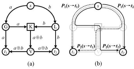
Figure 2 illustrates an example NCM scenario, where sourcesdelivers two bits, a and b, to two receivers, t1 and t2, respectively. The data transmission
150
scheme is shown in Figure 2 (a), where coding nodeK performs packet recom-bination a⊕b. Figure 2 (b) shows the four paths originating from source s
to one of the receivers. Note that, paths to the same receiver are link-disjoint paths. For example, paths P1(s → t1) and P2(s → t1) are link-disjoint. All
paths transmitting the NCM data form the NCM subgraph, as illustrated in
155
Figure 2 (b).
The following lists notations used in the paper:
• s: the source node in networkG(V, E);
• T = t1, t2, ..., td: the set of receivers, where d = |T| is the number of
receivers;
Figure 2: An example NCM scenario. (a) Data delivery. (b) The NCM subgraph.
• R: the data rate (an integer) at which sdelivers data toT;
• Pi(s, tk): thei-th path from stotk, wheretk ∈T andi= 1, ..., R;
• r(s, tk): the achievable data rate fromsto receivertk∈T;
• Ccode: the number of coding links inGN CM(s, T);
• clink(e): the cost incurred on linkeife∈GN CM(s, T);
165
• delay(Pi(s, tk)): the end-to-end delay of pathPi(s, tk).
The task is to find an appropriate NCM subgraph inG(V, E), which satisfies the NCM data rate requirement, with three objectives minimized, as shown below in Eq. 1.
Minimize:
f1=P∀e∈GN CM(s,T)clink(e) f2=Ccode
f3=1dP
d
k=1max{delay(Pi(s, tk))|i= 1, ..., R}
(1)
Subject to:
r(s, tk) =R,∀tk∈T (2)
In Eq. 1, objective f1 is to minimize the bandwidth resource, i.e. total
170
link cost involved during the NCM; objectivef2 is to minimize the computing
the average end-to-end delay along all paths in the NCM subgraph. Constraint 2 restricts thatRlink-disjoint paths are to be constructed fromsto each of the receivers so that the expected data rateRis achievable.
175
The above three-objective minimization problem belongs to MOPs. Sup-pose there are two solutions (f1∗, f2∗, f3∗) and (f10, f20, f30). (f1∗, f2∗, f3∗) dominates (f10, f20, f30) or (f10, f20, f30) is dominated by (f1∗, f2∗, f3∗) only if any of the following three conditions is satisfied: {f1∗ < f10, f2∗ ≤ f20, f3∗ ≤ f30} or {f1∗ ≤ f10, f2∗ < f20, f3∗ ≤f30} or {f1∗ ≤f10, f2∗≤f20, f3∗ < f30}. Optimal solutions to the problem
180
above constitute the Pareto-optimal Set (PS).
2.2. Related work-an overview
This subsection first reviews the main streams of NCM routing optimization problems in the literature.
(1) Optimization in NCM Routing
185
• Coding cost minimization. Performing coding operations consumes ex-tra computing resources, compared with the ex-traditional store-and-forward based routing. Hence, one research stream focuses on minimizing the amount of coding operations necessarily performed. Early research stud-ied greedy-based optimization approaches [8, 9]. Later on, several genetic
190
algorithms (GAs) were proposed for minimizing coding cost [10, 11, 12]. Recent research adapted estimation of distribution algorithms (EDAs), in-cluding quantum-inspired evolutionary algorithms (EAs) [13], population based incremental learning (PBIL) [14] and compact GA [15]. Moreover, EAs hybridized with other techniques, e.g. entropy-based evaluation
re-195
laxation and path-oriented encoding, were investigated [16, 17, 18, 19].
• Link cost minimization. NCM data are delivered through multiple paths which are made up of links [8]. In real networks, different links, when employed for data transmission, incur different costs, known as link costs. NCM routing plans with less total link costs are thus preferred. Lun
200
where wireline and wireless networks were both considered [20, 21, 22]. Cui and Ho studied the least-cost integral network coding problem, where the packet injection rate on each link was constrained to be integral [23]. Re-searchers also investigated minimum cost subgraph construction in static
205
and dynamic environments [24].
• Delay related optimization. Delay is one of the most important met-rics evaluating network performance. A considerable amount of applica-tions require guarantees on stringent delay, especially for real-time broad-band multimedia applications [25]. However, network coding gains high
210
bandwidth utilization at the expense of consuming extra computational resources at corresponding nodes [4]. Packet recombination (i.e. cod-ing operation) incurs additional processcod-ing delay in individual nodes, and cause severely large end-to-end delays if data are not routed appropriate-ly. Delay-related issues, when deploying practical NCM, have thus drawn
215
a great amount of attention. Delay analysis and its minimization have been studied in the context of wireless networks [26, 27], overlay networks [28], broadcast erasure channels with feedback [29, 30], instantly decodable network coding [31, 32, 33], and multicasting [34, 35].
• Multi-objective optimization. All the above research concerned
single-220
objective optimization problems. However, both coding and link costs incur in real-world NCM data delivery thus should be both minimized. This problem can be formulated as a bi-objective optimization problem, for which a number of multi-objective evolutionary algorithms (MOEAs) have been proposed [36, 37, 38, 39]. When launching NCM, Network
225
Service Providers (NSP) pay for computing and bandwidth resources they consume. Optimization on the two objectives helps NSPs to find a trade-off between the cost of paying the limited computing resource (coding) and bandwidth resource (link), to gain high profits. In addition, end users usually expect to have decent quality of experience (QoE), especially small
230
prefer less network resource consumption. In [40], the trade-offs between the total cost (i.e. weighted sum of the coding and link costs) and the maximum end-to-end delay of multiple paths were studied.
(2) MOEA/Ds integrated with other techniques
235
Incorporating sophisticated techniques into MOEA/D has become an im-portant direction in the MOEA/D family, including estimation of distribution algorithms, differential evolution, memetic algorithm, ant colony optimization and so on, as the following reviews.
• Estimation of distribution algorithm (EDA). Recently, EDAs gain
240
good attentions in solving various single-optimization problems (SOPs) [44]. In principle, they are a family of EAs that incorporate machine learning techniques, where statistical information of promising solutions is extracted to build probabilistic models, from which samples are generated. Compared with traditional EAs, EDAs usually obtain better optimization
245
results, with relatively less space and time complexity. A decomposition-based EDA, namely MEDA/D, is proposed to handle the multiobjective knapsack problems [45]. Shim et al. incorporated the restricted Boltz-mann machine and the evolutionary gradient search into the MOEA/D framework [46]. This algorithm performs well in addressing the
multiob-250
jective multiple traveling salesman problem (TSP). Gao et al. investigat-ed a similar problem, i.e. multiobjective TSP, using multiobjective EDA based on decomposition (MEDA/D) [47], where the probabilistic model is built based on priori and learnt information. To gain a balanced per-formance on global exploration and local exploitation, a hybrid adaptive
255
MOEA that synthesizes GA, EDA and DE was presented [48]. Promising solutions generated at an early stage of evolutions by these algorithms are used to produce corresponding proportion of solutions in the next genera-tion. Giagkiozis et al. developed a combination of MOEA/D and EDA for the many-objective optimization problems [49], where a novel generalized
decomposition method unifies different performance objectives. Ray et al. designed a hybridized architecture combining MOEA/D and quantum genetic algorithm for tackling many objective optimization problems [50], where systematic sampling is adopted to establish the reference directions and the evolution of quantum individuals is driven by a simple variation
265
operator.
• Differential evolution (DE). DE was integrated into the framework of MOEA/D in [51] to effectively handle complicated Pareto fronts for MOP-s, and it is reported to perform much better than NSGA-II. A variant of MOEA/D-DE was presented for the multi-objective analog cell sizing
270
problem [52]. Two performance enhancing mechanisms are incorporated to balance between the diversity and guiding information from neighbors, and to improve the local search ability of DE using a scaling factor. Tan et al. proposed a modified MOEA/D-DE with a uniform design method to generate uniformly distributed scalar optimization subproblems and a
275
simplified quadratic approximation to enhance the local exploitation and the accuracy of aggregation function values [53]. Combined with Gaus-sian mutation operators, MOEA/D-DE also has a decent performance in devising Yagi-Uda antennas [54]. Another variant of MOEA/D-DE, name-ly the adaptive DE for multiobjective problem (ADEMO/D), integrated
280
with a number of adaptive strategies, gains evenly distributed solutions well approximating the Pareto front for continuous MOPs [55, 56].
• Memetic algorithm (MA). Local search operators (assisted with do-main knowledge) have recently been incorporated into MOEA/D. With improved local exploitation, the proposed algorithms (usually called
multi-285
objective memetic algorithms) provide better solutions than pure MOEA/D. Chen et al. enhanced the performance of MOEA/D by integrating guided mutation and priority update [57]. Mei et al. proposed an MA/D with extended neighborhood search, namely D-MAENS, for solving the capac-itated arc routing problem [58]. Later on, Shang et al. improved the
performance of D-MAENS by two novel schemes, one for solution replace-ment and the other for elitism maintenance [59]. MOEA/D is hybridized with a mathematical programming technique (called Nelder and Mead’s algorithm), where Nelder and Mead’s algorithm serves as the local search mechanism [60]. Alhindi and Zhang investigated how guided local search
295
is used to strengthen MOEA/D in terms of escaping local optima [61]. Mashwani and Salhi presented a hybrid MOEA/D, where particle swarm optimization (PSO) and DE are incorporated. In the algorithm, DE acts as the main evolutionary framework and PSO is in charge of local search [62]. By combining ideas from MOEA/D and Pareto local search, Ke et al.
300
proposed a memetic algorithm based on decomposition (MOMAD) [63], where three populations are initialized by a problem-specific single objec-tive heuristic and evolved by the Pareto local search and single objecobjec-tive local search procedures. Ma et al. developed a MOEA/D with Baldwinian learning for continuous MOPs, where evolving information from the
dis-305
tribution model of the population is extracted by a Baldwinian learning operator [64].
• Ant colony optimization (ACO). Inspired by ACO, Li et al. in-troduced a probabilistic representation based on pheromone trails into MOEA/D and demonstrated its good potential in handling hard MOPs
310
with many local optima [65]. Ke et al. introduced the ACO into MOEA/D for solving multi-objective 0-1 knapsack problem and bi-objective TSP [66]. Instead of using sub-colonies, each ant solves one of the scalar opti-mization problems obtained. Cheng et al. proposed a hybrid multiobjec-tive optimization framework integrating the ACO into MOEA/D, called
315
MoACO/D [67], where an ant colony is divided into many sub-colonies in an overlapped manner, and each sub-colony addresses a certain SOP decomposed from the original MOP.
• Other techniques. A considerable amount of research efforts have al-so been made to incorporating various optimization techniques into the
MOEA/D framework. These include PSO [68, 69, 70], simulated anneal-ing [71], artificial bee colony optimization [73], fuzzy system [74], Gaussian process model [75], opposition-learning [76], teaching-learning algorithm [73, 77], and so on.
3. Overview of MOEA/D and PBIL
325
3.1. MOEA/D
In MOEA/D, the fundamental idea is to decompose a MOP intoN scalar optimization subproblems (SOSPs) [41]. MOEA/D aims to optimize all SOSPs simultaneously in a collaborative and time-efficient manner. Three decompo-sition methods are introduced in [41]. This paper considers the Tchebycheff approach, one of the most commonly used. A SOSP achieved by the decompo-sition of a MOP can be expressed as follows:
Minimize :g(x|λ, z∗) = max
1≤j≤m{λj|fj(x)−z
∗
j|} (3)
Subject to :x∈Ω (4)
where m is the number of objectives, λ = (λ1, ..., λm) is a weight vector, i.e.
λj ≥0, j = 1, ..., m, andP m
j=1λj = 1. z∗={z1∗, ..., zm∗}is the reference point,
i.e. z∗=min{fj(x)|x∈Ω}, where Ω is the decision space.
It is assumed that a set of N weight vectors λ1, ..., λN should be
select-330
ed properly so the optimal solutions of those SOSPs will well approximate the Pareto-optimal front (PF). In addition, the neighborhood relationship of SOSPs can be measured by Euclidean distances between the weight vectors. Neighbor-ing SOSPs have similar fitness landscapes and their optimal solutions should be close in the decision space. Information sharing between neighborhoods thus
335
can be exploited to accomplish the optimization task.
The evolutionary procedure of MOEA/D can be described below.
• A population ofNpointsx1, ..., xN ∈Ω, wherexiis the current individual
to SOSP(i), thei-th SOSP.
340
• z= (z1, ..., zm), wherezj, j= 1, ..., m, is the best-so-far value for objective
fj.
• An external population (EP), which stores nondominated solutions found during the search.
Input: a given MOP; stopping criteria;N: the number of SOSPs;W: the
345
number of the neighbors for each SOSP;λ1, ..., λN: uniformly distributed weight
vectors;pc: the crossover rate;pm: the mutation rate.
MOEA/D Procedure:
Initialization:
1: Set EP =∅.
350
2: For arbitrary weight vector λi, calculate the W closest weight vectors,
λi(1), ..., λi(W), via Euclidean distance and setϕ(i) ={i(1), ..., i(W)}.
3: Generate an initial populationx1, ..., xN and evaluatefu(xj) for each
indi-vidual.
4: Initializez={z1, ..., zm}.
355
Repeat:
5: fori= 1 toN do
6: Reproduction: Generate a new solution y by two individuals xu and
xlusing crossover and mutation operators, whereu, l∈ϕ(i).
7: Improvement: Improve y by using a problem-specific improvement
360
repair operator, which is optional.
8: Update of z: Forj = 1, ..., m, iffj(y)< zj, setzj =fj(y).
9: Update of neighboring solutions: For eachk∈ϕ(i), ifg(y|λk, z)≤
g(xk|λk, z), then setxk=y andfj(xk) =fj(y), j= 1, ..., m.
10: Update of EP: Remove those solutions dominated byy from EP and
365
Termination:
12: Until stopping criteria are satisfied, output EP.
3.2. PBIL
370
PBIL has been reported to gain promising performance when solving the single-objective network coding resource minimization problem [14]. Instead of using an explicit population, PBIL manipulates a real-valued probability vector (PV). When sampled, PV generates a number of binary solutions and the best one is used to update the PV. By making use of global information, promising
375
solutions are generated with increasingly higher probabilities stored in PV. LetP(k)={Pk
1, ..., PLk}be a PV at generationk, whereL is the dimension
of the solution encoding and Pk
l is the probability of obtaining ‘1’ at thel-th
position. DenoteB(k)={Bk
1, ..., BkL} andαthe best so far solution during the
search and the learning rate, respectively. Figure 3 shows the procedure of the
380
original PBIL. The PV at generationk,P(k), is updated by Eq. 5.
P(k)= (1.0−α)·P(k−1)+α·B(k) (5)
After PV is updated, mutation operation may be used to avoid local optima [72]. Letαbe the probability shifting at each position, andPk
l is to be mutated,
Eq. 6 is typically adopted in mutation.
Pl(k)= (1.0−σ)·Pl(k−1)+frnd·σ (6)
wherefrnd is either 0.0 or 1.0, randomly generated with probability 0.5.
385
4. The proposed MOEA/D-PBIL
As known, the individual representation is one of the most important issues in EAs. This section starts with the individual representation used for the problem concerned in this paper. Then, three novel features, i.e. a probability-based initialization scheme, a problem-specific population updating rule and a
390
Initialization:
1: Setk= 0. 2: SetPk
l = 0.5,l= 1, ..., L. SoP(k)is initialized as{0.5, ...,0.5}.
3: Sampling a set S(k) of N individuals from P(k) and find the best sample
andB(k).
Repeat:
4: Setk=k+ 1.
5: Find the best sampleB(k)fromB(k−1)∪S(k−1). 6: UpdateP(k) by Eq. 5.
7: MutateP(k)by Eq. 6.
8: Sampling a setS(k) ofN individuals from P(k). Termination:
9: Until stopping criteria are satisfied, outputB(k).
Figure 3: Procedure of the original PBIL [72]
4.1. Individual representation and evaluation
Binary link state individual representation (BLS-IR) has been widely used in network coding related optimization problems, including a number of
single-395
objective optimization problems and MOPs [10, 11, 12, 13, 14, 15, 19, 40]. In particular, BLS-IR is able to facilitate an easy process of estimating the consumption of the coding resource during the NCM data transmission. As mentioned before, coding operations can be performed at merging nodes only. BLS-IR is based on the graph decomposition method (GDM) which helps to
400
clearly show how information flows are forwarded within each merging node [11]. The MOP concerned in this paper also involves the estimation of coding resource consumption, so it is rationale to utilize BLS-IR to represent individuals. The following introduces GDM, BLS-IR and the raw fitness evaluation.
In GDM, each merging node M with IM incoming links and OM outgoing
405
links is decomposed intoIM incoming auxiliary nodes and OM outgoing
link flows into nodeM is redirected to one of theIM incoming auxiliary nodes,
and each node has only one link flows into it. Similarly, each outgoing link from nodeM is redirected to one of theOM outgoing auxiliary nodes and each node
410
has only one outgoing link. Besides, within each decomposed merging node, an auxiliary link connects each incoming auxiliary node with each outgoing aux-iliary node. Given an original graphG, every merging node is decomposed by GDM and then a decomposed graphG0 is created.
In BLS-IR, each individualxis represented by a string of binary variables,
415
each associated with an auxiliary link between auxiliary nodes. Value 1 for a binary variable means the corresponding link inG0is active and information can pass by; otherwise, the corresponding link inG0 is inactive and no information is allowed to pass. An individualxthus corresponds to an explicit and unique decomposed graph GD(x). Based on GD(x), we determine if a valid NCM
420
subgraph (see Section 2 for details) can be found.
The feasibility is firstly checked when evaluating an individualx. If a NCM subgraph from the corresponding decomposed graphGD(x) with the expected
data rate satisfied can be found,xis feasible; otherwise, it is regarded infeasible. One of the max-flow algorithms, the Goldberg algorithm, is used to calculate
425
the max flow between the source and each receiver within the obtained NCM subgraph [78]. For each feasible individual, three objective values are calculated according to Eq. 1. For infeasible individuals, three sufficiently large objective values are set, ensuring that infeasible individuals are less competitive than feasible ones during the evolutionary search procedure.
430
4.2. The probability-based initialization scheme
In MOEAs, the initial population generally has a great impact on the op-timization performance. Unfortunately, the problem concerned in the paper is highly constrained, and with BLS-IR, infeasible solutions dominate the search space. A random initial population very likely leads to a deteriorated
opti-435
1: Set initial population setinit = ∅ and probability vector P(init) =
{Pinit, Pinit, ..., Pinit}.
2: while|setinit|< N do
3: Gerenate a new individual xby samplingP(init) once. 4: if xis feasiblethen
5: Placexin setinit.
6: end if
7: end while
Figure 4: Pseudo code of the PBI scheme
of feasible individuals with high level of diversity.
In the literature, to deal with such problem, Kim et al. inserted an all-one individual into the initial population to ensure that the search starts with at least
440
one feasible solution [11, 12]. However, such method is not effective for MOPs, as MOEAs require higher level of population diversity than single-objective EAs. Therefore, our previous work investigated the estimated distribution of feasible solutions over the entire search space [40]. It was found that the majority of feasible solutions are closer to the all-one individual. Based on this finding, a
445
smart initialization scheme is proposed to generate an individual pool of multiple feasible individuals based on the all-one individual. However, such scheme leads to an initial population of highly similar individuals, which seriously harms the population diversity.
We use the concept of PV in PBIL to generate the initial population. The
450
distribution of feasible individuals in the search space is estimated to extract statistical information. Instead of setting each value in the PV to 0.5, we set a larger probability at each position of PV, to generate feasible individuals with a higher probability. Figure 4 shows the pseudo code of the PBI scheme. This is in compliance with the finding above, i.e. an individual similar to the all-one
455
individual is more likely to be feasible.
while considering its diversification. As long asPinitis not set too close to 1, the
initial population could maintain a certain degree of diversity. A smallerPinitis
more likely to gain a more diversified initial population, which is of course at the
460
expense of longer computational time. Since diversity is extremely important for MOEAs, it is worth compromising the computational cost.
4.3. A problem-specific population updating rule
In the original MOEA/D, a better individual replaces not only the best-so-far individual of the corresponding SOSP, but also those of neighboring SOSPs.
465
However, the problem concerned in the paper is highly complicated and con-strained, and feasible individuals only account for a very small proportion of the population [40]. In addition, the majority of feasible individuals are close to the all-one individual. If we adapt the original population updating rule, where better individual updates every SOSP within the same neighborhood, similar
470
individuals will rapidly dominate the population, cause serious prematurity and deteriorate the optimization performance.
To overcome the above problem, this paper proposes a problem-specific pop-ulation updating (PSPU) rule, where, instead of multiple SOSPs, only a single SOSP is updated with the newly generated promising individual. Let thei-th
475
SOSP be denoted by SOSP(i), where i= 1, ..., N. Let SOSPs(i) be the set of the neighbors of SOSP(i) including itself, where SOSPs(i) = {SOSP(i(1)), ..., SOSP(i(W))},i(1), ..., i(W)∈ϕ(i) (see Subsection 3.1 for details). For an arbi-trary SOSP(i), an individualyis generated after reproduction, and replaces the individual of a neighboring SOSP with the most significant fitness improvement.
480
Note that it is possible the newly generated individual is worse than all of the current individuals of SOSPs(i). In this case, the new one is discarded.
The fitness improvement of SOSP(i), ∆SOSP(i), and the most significant
improvement regarding the fitness among SOSPs(i), ∆max, are defined in Eq.
7 and Eq. 8, respectively.
485
∆max= max ∆SOSP(j), j∈ϕ(i) (8)
where,ϕ(i) contains the indexes of all SOSPs in SOSPs(i).
Compared with the original population updating rule in MOEA/D, the pro-posed PSPU rule defines that a newly generated individual updates the most appropriate SOSP only. Thus, the search is guided to explore promising areas in the search space while maintaining a diversified population. With the proposed
490
rule, MOEA/D-PBIL gains better performance as observed in Subsection 5.4.
4.4. A hybridized reproduction scheme
When designing MOEAs, the issue of exploration and exploitation at differ-ent stages of the search should be carefully considered to support effective search over the vast solution landscape. Traditional EA recombination operators, e.g.
495
crossover, recombine at least two individuals selected from the population, mak-ing use of the local information only. They perform well at the beginnmak-ing of the evolution, but get worse due to gradual loss of population diversity, leading to a deteriorated global search performance. PBIL manipulates a PV and generates new individuals by sampling from it. By making use of the global and
histori-500
cal information, promising regions can be explored in parallel and new regions also have chance to be discovered. An effective global exploration is obtained by the intrinsic memory of PV. The recombination of PBIL can thus act as a complement to the traditional EA recombination.
To achieve a balanced global exploration and local exploitation,
MOEA/D-505
PBIL utilizes a hybridized reproduction (HR) scheme which uses the genetic operators of MOEA/D and the probabilistic sampling operators of PBIL at different stages of the evolution. By controlling the proportion of the offspring produced by MOEA/D and those by PBIL, the proposed algorithm aims at striking a balanced global exploration and local exploitation. To be specific,
510
is more likely to be selected for concentrating on promising areas in the search space.
515
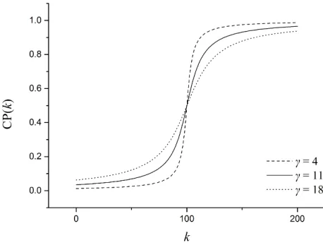
According to the HR scheme, we need a controlling parameter CP(k) for gen-erationkto determine how many individuals are generated by PBIL-reproduction. We find that the cumulative distribution function (CDF) of the Cauchy distri-bution can be adapted for controlling the PBIL offspring proportion, since the CDF curve grows gradually and smoothly from a value close to 0 to a value
520
close to 1 [79]. We thus define CP(k) in Eq. 9. This parameter determines which reproduction method is used to generate a new individual. For thei-th SOSP, if an uniformly distributed random numberrand≤CP(k), then PBIL-reproduction is chosen to produce offspring; otherwise, MOEA/D-PBIL-reproduction is chosen. If PBIL-reproduction cannot produce a feasible individual after a
525
predefined number of attempts, especially in the early stage of the evolution when building up the probabilistic blocks for the PV, MOEA/D-reproduction is used instead.
CP(k) = 1
πarctan(
k−K/2
γ ) +
1
2 (9)
where, parameter γ is a predefined value governing the steepness of the CP curve and parameterK is a predefined number of generations.
530
Figure 5 illustrates an example curve of CP, whereK is set to 200 and γis set to 4, 11, and 18, respectively. A smallerγ leads to a deeper slope (in the paper,γis fixed at 11). It is clear that at the early stage (k= 1−50), MOEA/D-reproduction is more likely to be chosen; during the middle stage (k= 51−150), the probability of selecting PBIL-reproduction gradually increases and becomes
535
higher than that of MOEA/D-reproduction after k = 100; at the last stage, individuals generated by PBIL-reproduction dominate the population. Using this controlling parameter, a balanced global exploration and local exploitation is obtained, leading to a decent performance as seen in Subsection 5.5.
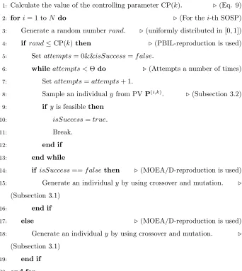
Figure 6 illustrates the procedure of the proposed HR scheme at generation
540
Figure 5: Example CP withK= 200 and different values ofγ
percentage of individuals each reproduction method generates at a certain gen-eration. Let the PV associated with thei-th SOSP at generationkdenoted by
P(i,k). Variable attempts is a counter, which records how many timesP(i,k)has
been sampled before a feasible individual appears. Variable ‘isSuccess’ records
545
the state whether PBIL-reproduction successfully produces a feasible individual. In the early stage of the search,P(i,k)focuses on learning probabilistic features
from promising samples. During this period, it is very likely that sampling
P(i,k) only results into infeasible individuals. The initial state of ‘isSuccess’
is set to false. Constant Θ stands for the maximum number of attempts tried
550
when samplingP(i,k). When PBIL-reproduction is chosen,P(i,k) is repeatedly sampled. This procedure stops when either a feasible individual appears or Θ attempts have been tried. If no feasible individual can be generated, we use MOEA/D-reproduction to produce a new individual.
The HR scheme has one significant advantage, i.e. helping to balance the
555
bal-1: Calculate the value of the controlling parameter CP(k). .(Eq. 9) 2: fori= 1 toN do .(For the i-th SOSP) 3: Generate a random numberrand. . (uniformly distributed in [0,1]) 4: if rand≤CP(k)then .(PBIL-reproduction is used) 5: Setattempts= 0&&isSuccess=f alse.
6: whileattempts <Θdo .(Attempts a number of times)
7: Setattempts=attempts+ 1.
8: Sample an individual yfrom PVP(i,k). . (Subsection 3.2)
9: if y is feasiblethen
10: isSuccess=true.
11: Break.
12: end if
13: end while
14: if isSuccess==f alsethen .(MOEA/D-reproduction is used) 15: Generate an individualy by using crossover and mutation. .
(Subsection 3.1)
16: end if
17: else .(MOEA/D-reproduction is used)
18: Generate an individualy by using crossover and mutation. .
(Subsection 3.1) 19: end if
20: end for
[image:24.612.136.478.181.564.2]Output: the offspring population.
anced performance between global exploration and local exploitation during all stages of the evolution, which is in favor of gaining an excellent optimization
560
performance.
4.5. The overall procedure of MOEA/D-PBIL
The proposed MOEA/D-PBIL is based on the basic evolutionary frame-work of MOEA/D (already reviewed in Subsection 3.1). Let k be the current generation of evolution. The following gives the whole evolutionary procedure.
565
Input:
• the MOP withmobjectives and individual lengthL; the stopping criteria; the population sizeN; the number of neighborsW; theN weight vectors
λ1, ..., λN; the crossover rate p
c; the mutation ratepm(Subsection 3.1)
• the learning rateα, the probability shiftingσ(Subsection 3.2)
570
• the probability for the PBI schemePinit (Subsection 4.2)
• the predefined number of generationsK; the predefined value for smooth-nessγin CP(k); the predefined number of attempts Θ (Subsection 4.4)
MOEA/D-PBIL Procedure:
Initialization:
575
1: Set EP =∅andk= 0.
2: Calculateϕ(i) neighbors for SOSP(i),i= 1, ..., N. . (Subsection 3.1) 3: Generate a populationx1, ..., xn by the PBI scheme. . (Subsection 4.2)
4: Initializez={z1, ..., zm}.
5: InitializeP(i,k)={Pk
1, ..., PLk},i= 1, ..., N. . (Subsection 3.2)
580
Repeat:
6: fori= 1 toN do
7: Reproduction: Produce an individualy by the HR scheme. .
(Subsection 4.4)
8: Update of z: For eachj∈ {1, ..., m}, iffj(y)< zj, setzj =fj(y).
9: Update of population: the PSPU rule is used to update the
popula-tion. . (Subsection
4.3)
10: Update of PV: Update P(i,k)by Eq. 5 and Eq. 6. . (Subsection 3.2) 11: Update of EP: Remove those solutions dominated byy from EP and
590
addy to EP if it is not dominated by anyone in EP. . (Subsection 3.1) 12: end for
Termination:
13: If stopping criteria are satisfied, stop and output EP.
In Step 3, the PBI scheme is used to generate an initial population, where
595
PV P(init) is repeatedly sampled in order to guarantee that every individual in the population is feasible. This provides the proposed algorithm a set of promising and diversified individuals to begin with. PBIL reproduction method is integrated into the MOEA/D framework (see Section 4.4). So, in the proposed algorithm, each SOSP is associated with a PV, e.g. P(i,k) = {Pk
1, ..., PLk}.
600
In Step 5, each PV is initialized as {0.5,0.5, ...,0.5}, where value ‘0.5’ is the probability of generating ‘1’ at that position. In Step 7, a new individual is produced by the MOEA/D- or PBIL- reproduction. In Step 9, the PSPU rule first calculates ∆maxaccording to Eq. 7 and Eq. 8. Forj∈ϕ(i), if ∆SOSP(j)=
∆max>0, then setxj=y andfu(xj) =fu(y),u= 1, ..., m, wherefu(x) is the
605
u-th objective value of individualx. No matter whether the PBIL reproduction method is chosen,P(i,k) is consistently updated at each generation, wherei= 1, ..., N. Step 10 defines the above procedure. In Step 13, the termination condition is that the algorithm evolves a predefined number of generations.
The learning rateαdefines how quickly PV learns from the best individual,
610
and has a great impact on the convergence of PV [72]. In MOEA/D-PBIL,
α is adaptively set during the evolutionary process. At the beginning of the evolution, as the quality of individuals is generally low, a smallαis set so that PVs could learn from promising individuals; during the evolution, the value ofα
is increased gradually until reaching to a maximal threshold (0.1 in this paper),
Table 1: Test Benchmark Networks and Their Parameters [40]
Networks
Parameters
nodes links receivers rate
7-copy 57 84 8 2
15-copy 121 180 16 2
Rnd-1 20 37 5 3
Rnd-2 20 39 5 3
Rnd-3 30 60 6 3
Rnd-4 30 69 6 3
Rnd-5 40 78 9 3
Rnd-6 40 85 9 4
Rnd-7 50 101 8 3
Rnd-8 50 118 10 4
which to some extent helps to provide a fine local exploitation.
5. Performance evaluation
This section studies the effectiveness of the three performance-enhancing schemes, i.e. the PBI scheme, the PSPU rule and the HR scheme, respectively, on benchmark test instances using certain performance metrics. The overall
620
performance of MOEA/D-PBIL is then evaluated, comparing against a number of state-of-the-art MOEAs, including NSGA-II [42] and SPEA2 [43].
5.1. Test instances
Ten widely used benchmark instances are considered in this paper, including two fixed networks (7-copy and 15-copy, see details in [18]) and eight randomly
625
generated networks (Rnd-1 to Rnd-8, with network size from 20 to 50, see details in [40]). The associated parameters of the ten instances are given in Table 1.
In the paper, for an arbitrary e∈E, its link costclink(e) and propagation
delay is uniformly distributed in the range of [5,15] and [2ms,10ms], respec-tively. The coding cost Ccode is the number of coding links in the obtained
630
network coding based multicast subgraph GN CM(s, T). We assume any
encourage scientific comparisons, the details of all instances can be found at http://www.cs.nott.ac.uk/ rxq/benchmarks.htm. The predefined number of generations for all algorithms for comparison is set to 200. All experiments
635
were run on a Windows 8 OS computer with Intel(R) Core(TM) i7-3740QM CPU 2.7 GHz and 8 GB RAM. The results are obtained by running each algo-rithm 20 times (unless stated otherwise), from which the statistics are collected and analyzed.
5.2. Performance measures
640
To thoroughly evaluate the performance of the proposed algorithm, we em-ploy five widely recognized performance measuring metrics throughout the ex-periments.
Let P Fref be a reference set of solutions well approximating the true PF,
andP Fknown be the set of nondominated solutions obtained by an algorithm.
645
Note that we may not know the true PF for highly complex multi-objective optimization problems, including the problem concerned in this work, so we combine the best-so-far solutions obtained by all algorithms after all runs and select the nondominated solutions as the reference set. This method has been widely adopted when evaluating multi-objective algorithms in the literature.
650
• Inverted generational distance (IGD) [41]: IGD is defined as the average distance from each pointv inP Fref to its nearest counterpart in
P Fknown, as follows:
IGD=
P
v∈P Fref
d(v, P Fknown)
|P Fref|
(10)
where d(v, P Fknown) is the Euclidean distance (in the objective domain)
between solution v in P Fref and its nearest solution in P Fknown and
|P Fref| is the number of solutions in P Fref. IGD measures the
conver-gence and diversity of an obtained nondominated solution set. This metric is commonly used to evaluate the overall performance of an algorithm. A
655
• Generational distance (GD)[80]: GD measures the average distance from each point v in P Fknown to its nearest counterpart in P Fref, as
defined below: GD= v u u t P
v∈P Fknown
d(v, P Fref)
|P Fknown|
(11)
where d(v, P Fref) is the Euclidean distance between v in P Fknown and
its nearest point in P Fref. This metric is used to measure how closely
P Fknown converges toP Fref. A smaller GD indicates the obtained PF is
closer to the true PF.
660
• Maximum spread (MS)[80]: MS reflects how well the true PF is cov-ered by the points in P Fknown through the hyperboxes formed by the
extreme function values observed inP Fref andP Fknown, as shown in Eq.
12.
M S=
v u u t 1 m m X i=1
(min(f
max
i , Fimax)−max(fimin, Fimin)
Fmax
i −F
min
i
)
2
(12)
wheremis the number of objectives;fmax
i andfiminare the maximum and
minimum values of thei-th objective inP Fknown, respectively; andFimax
and Fmin
i are the maximum and minimum values of the i-th objective
in P Fref, respectively. A larger MS shows the obtained PF has a better
spread.
665
• Average Computational Time (ACT): ACT is the average running time consumed by an algorithm over 20 runs. This metric is a direct indicator of the computational complexity of an algorithm being tested.
• Student’s t-test [79]: This test is to compare two algorithms in terms of the IGD values obtained in 20 runs. In this paper, two-tailed t-test
670
with 38 degrees of freedom at a 0.05 level of significance is used. The
5.3. The effectiveness of the PBI scheme
675
In general, an initial population should contain a considerable amount of di-verse and feasible individuals. A PBI scheme is proposed (see Subsection 4.2) to generate a set of feasible initial individuals, by repeatedly sampling an initial PV
P(init) ={P
init, Pinit, , Pinit} until a predefined number of feasible individuals
are created. The value ofPinit is of vital importance to the performance of the
680
PBI scheme. Three different settings are compared in the proposed scheme. Be-sides, the PBI scheme is also compared with two existing initialization schemes, i.e. Kim’s method [11] and Xing’s method [40], as listed below.
• Kim’s method [11]: the initial population is randomly generated. An all-one individual is included into the population to ensure the search
685
start with a feasible search point. It is widely used in the network coding resource minimization problem.
• Xing’s method [40]: one-bit mutation is performed on the all-one in-dividual and its variants to produce a set of feasible inin-dividuals that are very closely distributed around the all-one individual. This method has
690
been adopted in MOP with network coding.
• PBI: the proposed initialization scheme. Three settings, i.e. Pinit = 0.7,
0.8 and 0.9, are tested. For simplicity purpose, we represent them as PBI(0.7), PBI(0.8) and PBI(0.9), respectively. A larger Pinit leads to a
higher probability of generating ‘1’ at the corresponding position. This is
695
in compliance with the research findings in [40], that individuals closer to the all-one individual are more likely to be feasible.
As aforementioned, IGD reflects the overall performance of an algorithm re-garding the quality of the obtainedP Fknown. Hence, IGD is also used to
evalu-ate the initial population. We compare the three initialization methods using six
700
7 illustrates the comparisons among different initialization methods, where hor-izontal axis represents the IGD of each population and the vertical axis is the computational time consumed by each method.
[image:31.612.149.464.209.458.2]705
Figure 7: Comparisons among different initialization schemes w.r.t. IGD
It is clearly seen that the PBI scheme performs significantly better than the other two methods in terms of IGD. Kim’s method provides an initial population with at least a feasible individual. However, infeasible individuals still account for the majority of the population [40], thus the individuals in the objective domain are far away fromP Fref. Xing’s method produces a feasible population,
710
Table 2: Student’st-test results of A1, A2 and A3
Network A3↔A1 A3↔A2
Rnd-1 + ∼
Rnd-2 + ∼
Rnd-5 + +
Rnd-7 + +
Rnd-8 + +
7copy + +
Kim’s and Xing’s methods are simple, thus both consume a smaller amount of time in all instances. On the other hand, the computational cost of the PBI
715
scheme has a wide spread in different instances. The smallest time cost of PBI is comparable to that of Kim’s and Xing’s methods.
With regard to different settings ofPinit of the PBI scheme, it is easily seen
that PBI(0.7) and PBI(0.8) are better than PBI(0.9) in all instances. Sampling a P(init) with larger Pinit, tends to produce more feasible individuals.
There-720
fore, to produce the same number of individuals, smallerPinit takes more time.
On the contrary, however, it is more likely to form a diversified population (ac-cording to the studies in [72]), thus PBI(0.7) and PBI(0.8) have better IGD values than PBI(0.9). Considering not only the quality of the population, but more realistically, also the time efficiency, we hereafter set Pinit = 0.9 in the
725
experiments.
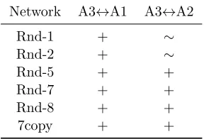
To further evaluate the superiority of the PBI scheme, we run the MOEA/D-PBIL with the three different initialization schemes, namely A1 with Kim’s method, A2 with Xing’s method and A3 with PBI(0.9), on the above six selected instances, results of Student’st-test shown in Table 2.
730
In Table 2, symbols ‘+’, ‘−’, and ‘∼’ in column A↔B indicate that algo-rithm A is significantly better than, significantly worse than, and statistically equivalent to algorithm B, respectively, in terms of the IGD. It is clear that A3 performs better than A2 and A1 in all instances. This also demonstrates that by providing the algorithm with a diversified and feasible population, the PBI
735
Table 3: Results of mean(SD) w.r.t. IGD, GD and MS (the best results are in bold) from A3
and A4.
Network IGD GD MS
A3 A4 A3 A4 A3 A4
Rnd-1 2.66(1.65) 1.85(1.39) 0.67(0.84) 0.47(0.74) 0.86(0.11) 0.83(0.02) Rnd-2 3.51(1.91) 1.96(1.36) 0.16(0.49) 0.08(0.35) 0.76(0.26) 0.89(0.10) Rnd-3 0.06(0.11) 0.02(0.03) 0.04(0.10) 0.00(0.00) 0.98(0.41) 0.99(0.02) Rnd-4 2.95(1.01) 2.79(0.69) 1.76(1.23) 1.58(0.66) 0.69(0.14) 0.78(0.06) Rnd-5 1.21(0.23) 0.90(0.23) 0.73(0.20) 0.72(0.25) 0.79(0.07) 0.87(0.08) Rnd-6 0.12(0.06) 0.11(0.07) 0.15(0.25) 0.10(0.21) 1.00(0.00) 1.00(0.00) Rnd-7 1.43(0.30) 1.37(0.13) 1.12(0.85) 0.62(0.38) 0.90(0.03) 0.99(0.01) Rnd-8 0.89(0.57) 0.69(0.45) 1.10(0.62) 0.79(0.63) 0.88(0.05) 0.90(0.05) 7copy 0.05(0.03) 0.03(0.02) 0.17(0.07) 0.13(0.02) 0.99(0.01) 0.99(0.01) 15copy 0.16(0.08) 0.12(0.05) 0.34(0.17) 0.22(0.04) 0.97(0.01) 0.97(0.01)
5.4. The effectiveness of the population updating rule
To evaluate the effectiveness of the PSPU rule (Subsection 4.3), we compare two MOEAs regarding the optimization results obtained, as listed below.
• A3: MOEA/D [41] with the PBI method, where the original population
740
updating rule is utilized
• A4: A3 with the PSPU rule
The optimization results in terms of the IGD, GD and MS are reported in Table 3. Not surprisingly, A4 clearly outperforms A3 regarding all measures in almost all instances, indicating the effectiveness of the PSPU rule. The design
745
of the proposed rule is in compliance with nature of the MOP being tackled, and to deal with the issue that the search space is dominated by infeasible individuals. Feasible individuals are difficult to generate during the evolution. So, when promising individuals appear, if no limitation is defined to update the population, their genes could be rapidly spread over the population within a few
750
Table 4: Student’st-test results of A3 and A4
Network Rnd-1 Rnd-2 Rnd-3 Rnd-4 Rnd-5 Rnd-6 Rnd-7 Rnd-8 7copy 15copy
A4↔A3 + + + ∼ ∼ + ∼ + ∼ +
Student’s t-test is conducted to compare A3 and A4, regarding IGD, GD and MS, and the results are shown in Table 4. A4 performs at least no worse,
755
often better than A3 (in more than half of the instances). This confirms the contribution of the PSPU rule to the proposed algorithm.
5.5. The effectiveness of the HR scheme
The HR scheme described in Subsection 4.4 adaptively uses one of the two reproduction methods, from MOEA/D and PBIL, to strike a balance between
760
global exploration and local exploitation during different stages of the evolution. The effectiveness of the HR scheme is evaluated by comparing the following two MOEAs.
• A4: Original MOEA/D with the PBI method and the PSPU rule
• A5: A4 with the HR scheme, i.e. the proposed MOEA/D-PBIL in this
765
paper
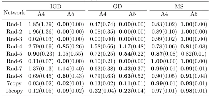
The results of IGD, GD, MS in Table 5, indicate that A5 outperforms A4 in 9 instances regarding IGD and GD and 6 instances in terms of MS, respectively. This demonstrates that the HR scheme in A5 helps to provide a decent global exploration and local exploitation during the evolution. On the other hand, the
770
global exploration ability gradually decreases in the original MOEA/D which only utilizes genetic operators for offspring reproduction, thus results into local optima solutions.
Results oft-test are in Table 6. A5 performs outstandingly better than A4, indicating the HR scheme greatly improves the performance of the proposed
775
Table 5: Results of mean(SD) (the best are in bold) from A4 and A5
Network
IGD GD MS
A4 A5 A4 A5 A4 A5
Rnd-1 1.85(1.39) 0.00(0.00) 0.47(0.74) 0.00(0.00) 0.83(0.02) 1.00(0.00) Rnd-2 1.96(1.36) 0.00(0.00) 0.08(0.35) 0.00(0.00) 0.89(0.10) 1.00(0.00) Rnd-3 0.02(0.03) 0.00(0.00) 0.00(0.00) 0.00(0.00) 0.99(0.02) 1.00(0.00) Rnd-4 2.79(0.69) 0.85(0.26) 1.58(0.66) 1.17(0.48) 0.78(0.06) 0.81(0.08) Rnd-5 0.90(0.23) 1.05(0.55) 0.72(0.25) 0.54(0.22) 0.87(0.08) 0.82(0.01) Rnd-6 0.11(0.07) 0.00(0.00) 0.10(0.21) 0.00(0.00) 1.00(0.00) 1.00(0.00) Rnd-7 1.37(0.13) 1.14(0.40) 0.62(0.38) 0.42(0.37) 0.99(0.01) 0.99(0.01) Rnd-8 0.69(0.45) 0.60(0.43) 0.79(0.63) 0.63(0.52) 0.90(0.05) 0.91(0.04) 7copy 0.03(0.02) 0.02(0.01) 0.13(0.02) 0.11(0.01) 0.99(0.01) 0.99(0.01) 15copy 0.12(0.05) 0.09(0.02) 0.22(0.04) 0.22(0.04) 0.97(0.01) 0.98(0.01)
Table 6: Student’st-test results of A4 and A5
Network Rnd-1 Rnd-2 Rnd-3 Rnd-4 Rnd-5 Rnd-6 Rnd-7 Rnd-8 7copy 15copy
A5↔A4 + + + + ∼ + ∼ ∼ + ∼
5.6. The overall performance evaluation
The proposed MOEA/D-PBIL algorithm is finally thoroughly investigated through performance comparisons against the following seven state-of-the-art MOEAs in the literature.
780
• NSGA-II: As one of the classical MOEAs originally proposed by Deb et al [42], NSGA-II is featured with three significant features, a fast non-dominated sorting approach, an elitism approach and a parameter-free diversity preservation scheme. We set the population size N = 100, the crossover rate pc = 0.9 and the mutation rate pm= 1/L, whereL is the
785
individual length.
• NSGA-II-Xing: With two improvements, i.e. Xing’s initialization method (in Subsection 5.3) and an individual delegation scheme in favor of diversi-fication, NSGA-II-Xing is able to gain promising optimization performance for the bi-objective MOP with network coding in our previous work [40].
• SPEA2: The strength Pareto evolutionary algorithm 2 [43] is another widely recognized MOEA. We denote the archive size by Narc and set
Narc=N = 100,pc= 0.9 andpm= 1/L, respectively.
• MOPSO: The multiobjective algorithm based on particle swarm intel-ligence [81] is well-known and widely used for performance comparison.
795
A population of 100 particles is maintained. We set pm = 1/L and 30
divisions for the adaptive grid.
• MOPBIL1: the multiobejctive PBIL proposed by Kim et al. has been re-ported to outperform a number of GA-based MOEAs when solving MOPs in the context of the robot soccer system [82]. When updating the i-th
800
PV, a solution randomly selected from the archive is used. Let the num-ber of PVs, the learning rate, and the amount of shift in the mutation be denoted by nP V, α, andσ, respectively. We set N = 100, Narc= 50,
nP V = 100,α= 0.15,pm= 0.02, andσ= 0.2.
• MOPBIL2: the first multiobejctive PBIL presented by Bureerat and
805
Sriworamas [83]. Thei-th PV is updated by 5 solutions randomly selected from the archive. We set N = 100, Narc = 50, nP V = 100, α = 0.15,
pm= 0.02, and σ= 0.2.
• MOEA/D: The original MOEA/D proposed by Zhang and Li (see Sub-section 3.1 for details) [41]. We set N = 100, pc = 0.9 andpm = 1/L,
810
respectively.
• MOEA/D-PBIL: The improved MOEA/D proposed in this paper. We setN = 100,Pinit= 0.9,r= 11,pc= 0.9 andpm= 1/L, respectively.
Results of IGD, GD, MS are collected in Tables 7, 8, and 9, respectively. In terms of IGD and GD, MOEA/D-PBIL performs the best, obtaining the
815
Table 7: Results of IGD (Best results are in bold) from the eight algorithms under comparison
Network Rnd-1 Rnd-2 Rnd-3 Rnd-4 Rnd-5 Rnd-6 Rnd-7 Rnd-8 7copy 15copy
NSGA-II 0.00 0.00 0.00 2.10 1.19 0.01 1.27 1.07 0.03 2.70 (0.00) (0.00) (0.00) (1.06) (0.30) (0.01) (0.29) (0.18) (0.01) (0.60) NSGA-II-Xing 0.00 0.00 0.00 0.85 1.14 0.00 1.21 1.09 0.03 2.56
(0.00) (0.00) (0.00) (0.26) (0.22) (0.00) (0.39) (0.20) (0.01) (0.53) SPEA2 5.27 5.68 0.92 3.97 1.73 2.07 3.57 1.46 0.08 2.20
(0.54) (0.86) (0.24) (3.39) (0.49) (1.13) (1.49) (0.36) (0.03) (0.61) MOPSO 3.08 3.51 0.82 2.20 1.97 1.77 2.65 3.78 0.54 7.30
(0.54) (1.87) (0.36) (0.39) (0.21) (0.34) (0.44) (0.33) (0.08) (1.39) MOPBIL1 0.00 0.44 0.00 0.69 1.15 1.08 1.11 1.07 0.05 3.15
(0.00) (0.17) (0.00) (0.59) (0.71) (0.48) (0.63) (0.58) (0.02) (2.63) MOPBIL2 0.42 0.63 0.00 0.78 1.24 0.82 1.54 1.07 0.06 3.02
(0.31) (0.23) (0.00) (0.65) (0.67) (0.26) (0.81) (0.59) (0.01) (1.87) MOEA/D 3.26 6.94 0.24 4.64 3.71 2.52 3.78 5.23 0.50 2.86
(0.34) (0.78) (0.09) (0.44) (0.43) (0.59) (0.76) (0.23) (0.41) (2.53) MOEA/D-PBIL 0.00 0.00 0.00 0.83 1.05 0.00 1.14 0.60 0.02 0.09
(0.00) (0.00) (0.00) (0.41) (0.55) (0.00) (0.40) (0.43) (0.01) (0.02)
and converged closer to the true PF, compared with those of other algorithms. MOEA/D-PBIL also achieves the best coverage of the true PF, and obtains the
820
highest MS in 8 instances (except Rnd-4 and Rnd-5 in Table 9). According to these three performance indicators, MOEA/D-PBIL gains the best performance in all instances due to the PBI scheme, PSPU rule, and HR scheme, which leads to a balanced trade-off between the global exploration and local exploitation, achieving better diversity and convergence at the same time.
825
Student’st-test between the 8 algorithms in Table 10 indicates that MOEA/D-PBIL is the best algorithm among all algorithms, performing no worse, and usually better than the others in most of the instances.
The results of ACT in Table 11 show that compared with the others, the orig-inal MOEA/D and MOEA/D-PBIL achieve the smallest ACTs in all instances.
830
Table 8: Results of GD (Best results are in bold) from the eight algorithms under comparison
Network Rnd-1 Rnd-2 Rnd-3 Rnd-4 Rnd-5 Rnd-6 Rnd-7 Rnd-8 7copy 15copy
NSGA-II 0.00 0.00 0.00 0.87 0.81 0.01 1.59 1.49 0.27 2.02 (0.00) (0.00) (0.00) (0.98) (0.16) (0.01) (0.82) (0.19) (0.07) (0.35) NSGA-II-Xing 0.00 0.00 0.00 0.81 0.88 0.00 1.36 1.29 0.21 1.82
(0.00) (0.00) (0.00) (0.79) (0.19) (0.00) (0.89) (0.25) (0.07) (0.27) SPEA2 0.31 0.40 0.10 2.75 0.94 1.53 0.80 0.41 0.37 2.02
(0.53) (0.68) (0.14) (2.54) (0.23) (1.04) (0.99) (0.27) (0.14) (0.37) MOPSO 0.56 0.71 0.19 2.93 1.54 1.72 1.96 2.56 1.24 3.26
(0.62) (0.79) (0.13) (1.00) (0.35) (0.22) (0.63) (0.53) (0.16) (0.22) MOPBIL1 (0.00) (0.02) (0.00) (0.33) (0.39) (0.57) (1.52) (0.75) (0.24) (1.02)0.00 0.02 0.00 0.35 0.82 0.84 2.20 1.05 0.30 1.92
MOPBIL2 0.30 0.05 0.00 0.60 0.87 0.75 2.05 1.03 0.27 1.88 (0.37) (0.02) (0.00) (0.53) (0.41) (0.32) (1.79) (0.86) (0.19) (1.15) MOEA/D 2.33 2.13 1.62 3.85 1.30 1.84 3.07 2.30 2.22 3.01
(0.42) (1.11) (0.37) (0.22) (0.18) (0.71) (0.34) (0.18) (0.20) (0.14) MOEA/D-PBIL(0.00) (0.00) (0.00) (0.48) (0.22) (0.00) (0.37) (0.52) (0.01) (0.04)0.00 0.00 0.00 1.17 0.54 0.00 0.42 0.63 0.11 0.22
Table 9: Result of MS (Best results are in bold) from the eight algorithms under comparison
Network Rnd-1 Rnd-2 Rnd-3 Rnd-4 Rnd-5 Rnd-6 Rnd-7 Rnd-8 7copy 15copy
NSGA-II 1.00 1.00 1.00 0.81 0.85 0.98 0.90 0.63 0.99 0.54 (0.00) (0.00) (0.00) (0.08) (0.07) (0.01) (0.04) (0.02) (0.01) (0.04) NSGA-II-Xing (0.00) (0.00) (0.00) (0.04) (0.04) (0.00) (0.03) (0.02) (0.01) (0.03)1.00 1.00 1.00 0.92 0.90 1.00 0.91 0.86 0.99 0.55
SPEA2 0.99 0.99 0.99 0.86 0.87 0.77 0.90 0.84 0.99 0.57 (0.04) (0.04) (0.01) (0.06) (0.07) (0.09) (0.02) (0.03) (0.01) (0.06) MOPSO 0.69 0.74 0.82 0.63 0.53 0.71 0.68 0.63 0.47 0.71
(0.13) (0.03) (0.08) (0.01) (0.06) (0.03) (0.03) (0.02) (0.04) (0.03) MOPBIL1 (0.00) (0.01) (0.00) (0.02) (0.06) (0.09) (0.03) (0.08) (0.02) (0.13)1.00 0.97 1.00 0.98 0.89 0.81 0.94 0.85 0.98 0.50
MOPBIL2 1.00 0.95 1.00 0.96 0.87 0.84 0.93 0.85 0.98 0.51 (0.00) (0.02) (0.00) (0.03) (0.08) (0.12) (0.03) (0.09) (0.01) (0.11) MOEA/D 0.67 0.72 0.80 0.63 0.52 0.71 0.51 0.63 0.47 0.69
[image:38.612.135.496.433.658.2]Table 10: Student’st-test results of the eight algorithms under comparison
Network Rnd-1 Rnd-2 Rnd-3 Rnd-4 Rnd-5
MOEA/D-PBIL↔NSGA-II ∼ ∼ ∼ + +
MOEA/D-PBIL↔NSGA-II-Xing ∼ ∼ ∼ + +
MOEA/D-PBIL↔SPEA2 + + + + +
MOEA/D-PBIL↔MOPSO + + + + +
MOEA/D-PBIL↔MOPBIL1 ∼ + ∼ ∼ +
MOEA/D-PBIL↔MOPBIL2 + + ∼ ∼ +
MOEA/D-PBIL↔MOEA/D + + + + +
Rnd-6 Rnd-7 Rnd-8 7copy 15copy
MOEA/D-PBIL↔NSGA-II ∼ + + + +
MOEA/D-PBIL↔NSGA-II-Xing ∼ + + ∼ +
MOEA/D-PBIL↔SPEA2 + + + + +
MOEA/D-PBIL↔MOPSO + + + + +
MOEA/D-PBIL↔MOPBIL1 + ∼ + + +
MOEA/D-PBIL↔MOPBIL2 + + + + +
MOEA/D-PBIL↔MOEA/D + + + + +
time to improve the optimization performance. MOEA/D-PBIL compared with
835
other MOEAs (except the original MOEA/D) demonstrates its efficiency.
6. Conclusions
This paper formulated a multi-objective optimization problem in the con-text of multicasting with network coding, where the three objectives, namely the coding cost, link cost and the end-to-end delay are minimized
simultaneous-840
ly. By analyzing the property of the search space, population-based incremental learning (PBIL) components were incorporated into the evolutionary framework, and a modified multi-objective evolutionary algorithm based on decomposition (MOEA/D-PBIL) was proposed. Three performance-enhancing schemes were developed, namely, the probability-based initialization scheme, the hybridized
845
ex-Table 11: Result of ACT (Sec.) (Best results are in bold) from the eight algorithms under
comparison
Network Rnd-1 Rnd-2 Rnd-3 Rnd-4 Rnd-5 NSGA-II 15.51 23.83 60.52 60.93 92.33 NSGA-II-Xing 15.08 23.53 58.85 60.95 90.50 SPEA2 9.66 17.73 34.01 48.87 77.55 MOPSO 28.38 25.94 27.38 178.60 228.54 MOPBIL1 9.21 17.22 36.71 62.72 80.05 MOPBIL2 9.36 18.90 36.86 64.37 86.03 MOEA/D 5.02 6.88 17.37 16.59 31.05
MOEA/D-PBIL 5.64 7.06 17.15 34.23 34.34 Rnd-6 Rnd-7 Rnd-8 7copy 15copy NSGA-II 67.55 195.37 265.49 95.57 909.79 NSGA-II-Xing 67.37 195.24 276.85 94.22 884.97 SPEA2 44.33 223.00 239.36 87.50 938.81 MOPSO 26.84 501.15 782.50 182.00 1603.45 MOPBIL1 45.95 148.50 289.39 91.11 869.67 MOPBIL2 48.61 146.36 298.66 93.80 846.94 MOEA/D 18.03 37.31 66.59 29.79 210.79
[image:40.612.160.451.292.538.2]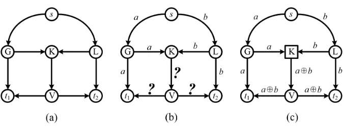
![Table 1: Test Benchmark Networks and Their Parameters [40]](https://thumb-us.123doks.com/thumbv2/123dok_us/8591372.371071/27.612.203.409.146.305/table-test-benchmark-networks-parameters.webp)