Can the removal of molecular cloud envelopes by external feedback
affect the efficiency of star formation?
William E. Lucas
1?, Ian A. Bonnell
1and Duncan H. Forgan
11SUPA, School of Physics & Astronomy, University of St Andrews, North Haugh, St Andrews, Fife KY16 9SS, United Kingdom
16 January 2017
ABSTRACT
We investigate how star formation efficiency can be significantly decreased by the removal of a molecular cloud’s envelope by feedback from an external source. Feedback from star formation has difficulties halting the process in dense gas but can easily remove the less dense and warmer envelopes where star formation does not occur. However, the envelopes can play an important role keeping their host clouds bound by deepening the gravitational potential and providing a constraining pressure boundary. We use numerical simulations to show that removal of the cloud envelopes results in all cases in a fall in the star formation efficiency (SFE). At1.38free-fall times our4 pccloud simulation experienced a drop in the SFE from 16 to six percent, while our5 pccloud fell from 27 to 16 per cent. At the same time, our3 pc cloud (the least bound) fell from an SFE of5.67per cent to zero when the envelope was lost. The star formation efficiency per free-fall time varied from zero to≈ 0.25according toα, defined to be the ratio of the kinetic plus thermal to gravitational energy, and irrespective of the absolute star forming mass available. Furthermore the fall in SFE associated with the loss of the envelope is found to even occur at later times. We conclude that the SFE will always fall should a star forming cloud lose its envelope due to stellar feedback, with less bound clouds suffering the greatest decrease.
Key words: stars: formation – ISM: clouds – accretion, accretion discs – hydrodynamics
1 INTRODUCTION
Star formation is a complex process governed by several inter-twined physical processes (Evans et al. 1999; Dobbs et al. 2014). The core mechanism is the collapse under gravity of dense regions of gas into stars, with this for the most part taking place in giant molecular clouds with only around ten per cent of stars forming in isolation (Lada & Lada 2003; Evans et al. 2009). Opposing this are thermal pressure along with turbulent kinetic motions (Heyer & Brunt 2004; Mac Low & Klessen 2004) and magnetic fields (Price & Bate 2009; Padoan & Nordlund 2011). The confluence of these processes governs the properties of a new stellar population such as the number of stars, their masses, locations, multiplicity and dy-namics (Shu, Adams & Lizano 1987; Bonnell, Larson & Zinnecker 2007).
One of the most important questions concerning star forma-tion is why it is so inefficient, with of order a few percent of the gas available on large scales being transformed into stars (Kenni-cutt & Evans 2012; Krumholz 2014; Heyer et al. 2016). Feedback from young stars, in the form of ionizing radiation, stellar winds or supernova explosions, is often invoked as a solution, but numeri-cal simulations have repeatedly shown that feedback has at most a moderate effect on the star formation efficiency of dense gas (Dale,
? E-mail: [email protected]
Bonnell & Whitworth 2007 and other papers in this series; Dale et al. 2014; MacLachlan et al. 2015). The effect is much more signif-icant in lower density gas, but it is instead in the higher density gas that star formation takes place. This would seem to indicate that feedback cannot greatly impact the efficiency of star formation.
In reality star formation takes place in dense and cold molec-ular hydrogen gas at the centre of these clouds. The optical depth here is high enough that they are shielded from the external Galactic radiation field, while the outer layers of the cloud are exposed and form an envelope of atomic hydrogen (Abgrall et al. 1992; Le Bour-lot et al. 1993). Observations of star forming clouds have found them to typically be marginally bound, though the virial parame-ter for individual clouds varies from0.1to10(Bolatto et al. 2008; Heyer et al. 2009; Wong et al. 2011; Dobbs et al. 2011; Dobbs et al. 2014).
corre-2
W. E. Lucas et al.
lation between SFE and density. Elmegreen & Lada (1977) intro-duced the concept of sequential star formation taking place as ion-izing feedback from young stellar clusters repeatedly sweeps up material to form new clusters. As such we ask how the SFE might change with the loss of a cloud’s envelope due to feedback in a similar scenario, though with the feedback here taking a negative rather than positive form.
Observations and models agree that the transition from warm low density gas to cold high density gas is gradual and that there is a mixture of phases present (Goldsmith & Li 2005). To test the envelope’s effect on star formation efficiency, we envision a sim-plified geometry with a warmer low density envelope surrounding the cold, dense and turbulent gas where star formation can occur. The extra gravity and pressure from the envelope keeps the super-virial cloud from expanding. Two scenarios follow: one in which the envelope remains in place, and one in which it is later removed as a first order approximation to its stripping by stellar feedback. In this paper we report on simulations of such a cloud within a transient warm envelope in order to ask whether such feedback can contribute to a significant reduction in the star formation efficiency in the dense gas.
2 NUMERICAL METHOD
Smoothed particle hydrodynamics (SPH) is a Lagrangian technique used to model a fluid as a set of particles. Each particle’s mass is spread throughout a volume with the use of a smoothing ker-nel. The fluid equations may then be reformulated as sums over the particles by treating the density, internal energy and so on as interpolated quantities. The simulations shown later in this paper were performed with the SPH codeSPHNG (Bate, Bonnell & Price 1995; Price & Monaghan 2007). This code allows for the creation of sink particles which represent stars. As a Lagrangian method, SPH also allows for mass to be traced throughout a simulation. This makes the method widely used in astrophysics, and as such many papers provide in-depth descriptions. Some recommendations are Benz (1990) and Monaghan (1992) for basic overviews, and Price & Monaghan (2004) for details of the grad-h formalism which was used here.
The basic simulation setup is as follows. Firstly, a spherical cloud of radius5 pcand mass104M
was created. The original
density was uniform with a value ofρ0 = 1.29×10⁻²¹g cm−3,
giving a free-fall time of1.85×106years. Its temperature was
set to10 K. The region from5to10 pcwas then filled with gas at103Kand a density a factor of ten lower then the inner cloud.
The sound speed in the cold inner cloud was0.253 km s−1while in the warm outer envelope it was2.53 km s−1. Note that the gas in both structures has a mean molecular weight of1.29, that for a mix of atomic hydrogen and helium, and differs only in temperature. Allowing it to change with phase would be desirable for a ‘com-plete’ simulation, but here it is kept constant both as a numerical convenience and in order to keep the model simple. From this point the terms ‘cloud’ and ‘envelope’ will refer to the inner and outer structures respectively.
A turbulent velocity field following an approximately Kol-mogorov power spectrum ofh|vk|2i ∝ k−3.5 was applied to the
[image:2.595.312.535.194.307.2]cloud. Theαvalue (Boss & Bodenheimer 1979) is the ratio of the kinetic plus thermal energy to the gravitational binding energy. The velocities were scaled such that, when considering the cloud in iso-lation, it would be unbound withα= 2.00. As such the root mean square (RMS) speed was4.53 km s−1(Mach numberM= 17.9),
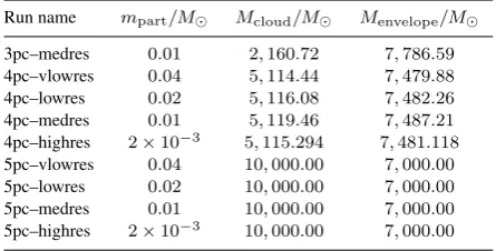
Table 1.The simulation names and meanings. The name reflects the cloud radius in parsecs and the resolution of the simulation (very low, low, medium or high). The second column gives the gas particle mass in solar units. The final two columns provide the mass of the cloud and envelope. Each run had two variations – one in which the warm envelope remained for the whole simulation’s duration (indicated by prefixing the name given here with an ‘E’) and another in which it was removed after a quarter of the cloud’s crossing time (indicated by ‘X’).
Run name mpart/M Mcloud/M Menvelope/M 3pc–medres 0.01 2,160.72 7,786.59 4pc–vlowres 0.04 5,114.44 7,479.88 4pc–lowres 0.02 5,116.08 7,482.26 4pc–medres 0.01 5,119.46 7,487.21 4pc–highres 2×10⁻³ 5,115.294 7,481.118 5pc–vlowres 0.04 10,000.00 7,000.00 5pc–lowres 0.02 10,000.00 7,000.00 5pc–medres 0.01 10,000.00 7,000.00 5pc–highres 2×10⁻³ 10,000.00 7,000.00
a value slightly above the3to 4 km s−1 that might be expected
for a cloud of this size and mass from the Larson relations (Larson 1981; Rosolowsky et al. 2003).
The envelope on the other hand was allowed to remain with no internal motions. Either thermal or ram pressure from the envelope could have been used to constrain the cloud, so while it was set to a temperature of103K, a lower value could have been used and the envelope also made turbulent. For simplicity, we used thermal pressure alone.
The same simulation was run with a less bound cloud by tak-ing the original cloud of radius5 pcand removing the layer from4
to5 pc, then recreating the envelope by populating the region from
4to10 pcwith low density warm gas as before. This left the cold cloud with a mass of5120M, and as such in isolationα= 3.15.
The4 and 5 pc setups were created at four resolution levels of
0.04M,0.02M,0.01M, and2×10−3Mper particle. Due to
the initial random particle placement, the total cloud mass did vary very slightly between different resolution simulations when deriv-ing the4 pcclouds. A single simulation was similarly set up to run with a cloud size of3 pcat the0.01Mresolution level. With a
mass of2160M, this cloud was most unbound withα= 5.59.
Dynamic sink particle creation was enabled in all simulations. The criteria for creation are as described in Bate et al. (1995); a brief description follows here. A gas particle being tested had to exceed a critical density set to108ρ0 = 1.29×10⁻¹³g cm−3,
and all its neighbours (gas particles within the kernel) had to be within a distance of0.01 pc. This clump of particles also had to be bound and collapsing. The SPH code aimed to give each particle around 50 neighbours and so the minimum sink mass was2M
in the ‘vlowres’ simulations,1Min ‘lowres’ simulations,0.5M
in ‘medres’ runs, and0.1Min ‘highres’. After sink creation, gas
particles within the same distance of0.01 pccould be accreted if it they passed a boundedness test. Particles within2.5×10−3pc
were accreted without testing.
After setup, the simulations were evolved isothermally un-der self-gravity for as long as possible before being halted by the small timesteps required in the high density regions forming sinks. For each, split simulations were created after a quarter of the tur-bulent crossing time in the cloud (evaluating to0.32 Myrfor the
3 pccloud,0.43 Myrfor the4 pccloud and0.54 Myrfor the5 pc
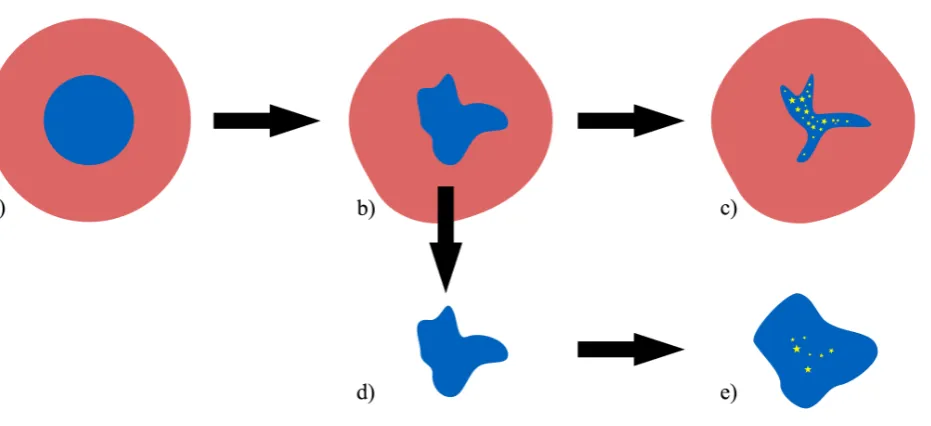
simu-Figure 1.Simulation method. In subfigure a), a cold turbulent cloud (blue) is embedded within a warm nonturbulent envelope (red). This was then evolved forwards in time, shown in subfigures b) and then c). Part of the way through the simulation, usually at a quarter of the turbulent crossing time and here shown in b), a separate simulation was created by removing the warm envelope to create the setup seen in subfigure d). The cloud was then evolved in isolation to a later time shown in e) to allow a direct comparison with the original run in which the envelope was retained for the entire duration of the simulation. It was expected that the loss of the envelope would lead to more star formation taking place in c) than in e). (A colour version of this plot is available in the online version.)
lations the envelope was removed from the medium resolution4 pc
cloud at later times of up to1.50tff. The process of evolution and
[image:3.595.66.532.101.314.2]creation of a parallel simulation without the envelope is shown in Figure 1.
The simulations and naming conventions are given in Table 1. The cloud radius in parsecs is provided, along with an indication of the resolution level of the simulation: very low, low, medium or high. When referring to a specific simulation, an ‘E’ is prefixed to this to indicate that the envelope remained throughout the whole simulation, while an ‘X’ prefix indicates that it was removed during the evolution.
3 EVOLUTIONARY OVERVIEW
As might be expected, the cold inner cloud’s evolution was char-acterised by the growth of overdensities throughout its evolution. These initially came about through the generation of structure via turbulence. Self-gravity was then able to take hold in the densest regions and bring them to the point where stars could be formed.
The warm envelope, retained in the E- simulations, maintained a roughly spherical symmetry as it gained little kinetic energy from the turbulent central cloud, and thus lacked significant internal motions. In contrast the cloud itself developed strong filamentary structure along with a number of sub-parsec scale clumps contain-ing dynamically formcontain-ing sink particles. As the cloud was by design unbound, it expanded and partially displaced the envelope.
The X- simulations, in which the envelope was removed, ex-hibit quite different evolution. As was noted in Section 2, they were removed at 0.25tcross once the turbulence had already started to
generate the internal filamentary structure. In the absence of the envelope the cold cloud was free to expand. The filaments formed from the turbulence were more diffuse in comparison with the sim-ulations in which the envelope was present throughout. This lower
density translates to a decrease in the importance of self-gravity and hence a decrease in the local star formation rate. As such par-allels in structure can be seen with the corresponding E- runs, but the small dense clumps seen previously did not form in these sim-ulations.
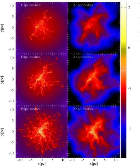
Figure 3 shows column densities and sink locations for the medium resolution simulations at all three cloud sizes (3, 4 and
5 pc) and both with and without the envelope, at 1.38tff =
2.54 Myr. Across the three cloud sizes, the most apparent change is the correlation of the original cloud size with the extent of dense structured gas after evolution. Much of this takes the form of cometary blobs of cold gas launched outwards through the en-velope. It is also immediately apparent that with the removal of the envelope in the E- runs, the ability of the cloud to form dense struc-ture in general along with sink particles dropped dramatically. At the same time, while the5 pccloud (the most bound of the set) was able to form stars in the absence of the envelope, the3 pccloud had failed to form any. Indeed no sinks had been formed even by the end of E3pc–medres at2.54tff= 4.71 Myr. E4pc–medres and
X4pc–medres lay between the extrema of the3and5 pcruns. Examining the density PDFs reveals in more detail the quanti-tative differences between the simulations. These are shown in Fig-ure 4 for the cold gas in the E- and X- variations of the 3pc–medres, 4pc–medres and 5pc–medres simulations at1.38tff.
4
W. E. Lucas et al.
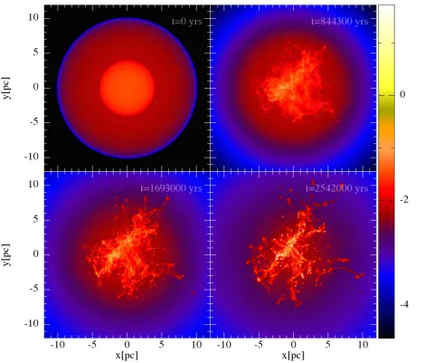
Figure 2. Evolution of simulation E4pc–medres. Shown are the column densities and sink particles (as white points) at four times. For reference, 844300 years = 0.46tff,1693000 years = 0.92tffand2542000 years = 1.38tff. Turbulence in the cloud generated structure, with sink particles forming
in the densest regions by the final time shown. Enough kinetic energy had been placed within the initial cloud to launch small blobs outwards, but with the presence of the envelope the cloud on the whole remained roughly the same size throughout. (A colour version of this plot is available in the online version.)
X5pc–medres, the same expansion is seen in gas moving to lower densities – at the same time, the cloud in this simulation was closer to being globally bound, and examination of the simulations does show that the central region was undergoing collapse. This resulted in the ‘flat-top’ of the density PDF for X5pc–medres, represent-ing the dense inner regions of the cloud as well as a new envelope formed from the expansion of its outer layers.
At the time of the PDFs shown in Figure 4, the median density in E3pc–medres was1.97×10−20g cm−3, while removing the
en-velope led to the median density in X3pc–medres falling to1.42×
10−22g cm−3. In E4pc–medres it was2.19×10−20g cm−3, while it similarly fell in X4pc–medres to4.00×10−22g cm−3. Finally the respective values for E5pc–medres and X5pc–medres were
2.58×10⁻²⁰g cm−3
and1.29×10−21g cm−3
.
Two observations may be made here. Firstly, changing the size of the cloud from3to5 pcled to only a small change in the median density in the E- simulations, while in the X- simulations it fell by almost a factor of ten. Secondly, removing the envelope dropped the median density by a factor of20in the 5pc–medres simulations but
a factor of55for the 4pc–medres runs and139for the 3pc–medres runs. That is to say, the density in the cloud was increased more by retaining the envelope than by making it larger and more bound. Thus we can say that the effect of the warm envelope contributed greatly towards maintaining higher densities in the cloud.
Approaching1tff, sink particles began to form in all
simu-lations with the exception of X3pc–medres, concentrated in the cold and dense filaments and clumps. In no simulation did enve-lope particles take part in accretion to sink particles. Over time the proto-clusters coalesced to form larger structures following a pro-cess similar to that seen in Bonnell, Bate & Vine (2003), the largest forming from the dense central regions of the cloud that can be seen just above the origin in Figure 3. Isolated sinks also formed from the smaller clumps at larger distances from the origin, but due to the clumps’ absence, at a much lower rate in the X- simulations in which the envelope had been removed.
Figure 3.Column densities for all medium resolution simulations at1.38tff = 2.54 Myr, with dots showing the locations of sink particles. The plots are
6
W. E. Lucas et al.
Figure 4. Mass-weighted density PDF of cold (10 K) gas in the 3pc– medres, 4pc–medres and 5pc–medres simulations at1.38tff = 2.54 Myr.
The dotted vertical line shows the original mean densityρ0 = 1.29×
10−21g cm−3in the cold gas. Aside from the difference in densities
be-tween the three sets caused by the increase of mass with cloud size, it is apparent that densities were enhanced when the warm envelope remained in place throughout the simulation. (A colour version of this plot is available in the online version.)
of sinks formed is likely an upper limit, with the true value being lower. However the simulations should still provide a good estimate of the total mass in stars, and it is with this quantity we investigate the star formation efficiency in the next section.
4 STAR FORMATION EFFICIENCY
The star formation efficiency (SFE) was found to be very different between the various simulations. The SFE was defined in relation to the mass of cold (10 K) gas in the cloud,Mcloud, a value
differ-ing between the variously-sized clouds used. It may then be simply calculated at any time by
SF E= Msinks
Mcloud+Msinks
, (1)
whereMsinksis the total mass in sink particles. As no envelope
par-ticles went into any sinks, the sum on the bottom always equalled the original cloud mass. Although the sink particles are only nu-merical representations of stars, they are a suitable proxy to allow the calculation of the SFE: while each one may not truly represent a star, it does still contain gas that was determined to be dense and gravitationally bound. As such, the SFEs reported here do repre-sent the star forming capability of the cloud, within the limits of the resolution, which is covered in Section 4.2.
4.1 Original simulations
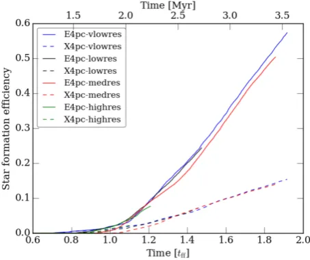
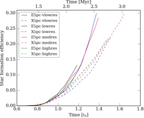
The SFEs of the4 pcclouds are plotted against time in Figure 5 for both the E- and X- variants and at all four resolutions used for that setup. A similar plot is shown for the5 pcclouds in Figure 6.
The profiles of the SFE for the two cloud sizes shown in Fig-ures 5 and 6 both follow a similar pattern. Before ≈ 1.0tff star
Figure 5.Star formation efficiency for the4 pcradius clouds. The low res-olution simulations actually began forming sink particles earlier than the medium resolution runs, but at such low rates that the SFE was of order 0.01. Once the SFE reached an appreciable fraction of unity, the runs at various resolutions had essentially diverged to give two groups: the E- runs in which the envelope remained in place throughout, and the X- in which it was removed. By the endpoints of these runs, the E- simulations had an SFE a factor of almost four greater. (A colour version of this plot is available in the online version.)
formation proceeded but very slowly. After that point the SFE in-creased much more quickly to sizeable fractions of unity, with the efficiencies for the E- and X- simulations beginning to diverge shortly afterwards at≈1.1tff. After this point the two sets of SFEs
continued to increase at roughly linear rates. The divergence ap-pears more noticeable for the4 pccloud thanks to the longer run-times that could be achieved for these simulations.
It is clear from both figures that the X- runs in which the warm envelope was removed were less efficient at forming stars when compared to the E- simulations in which the envelope remained throughout the simulation. Taking a fiducial point at1.38tff, the
SFE in E4pc–medres was 0.16 while it fell to 0.06 in X4pc– medres. At the same time for the5 pc, E5pc–medres had an SFE of
0.27and X5pc–medres had0.16. By the latest times available for the4 pccloud, after1.8tff, the difference was even greater, with
theSFE ≈ 0.15in the X- runs increasing to over0.5in the E-runs.
Though the values are too low to be seen in the figures, star formation began in the4 pccloud at different times, from0.7to just over1tff depending on the level of resolution and whether
the envelope was present or not. Conversely, star formation in the
5 pccloud began between0.7and0.8tffin all cases. An
observa-tion may be made in that all the simulaobserva-tions in which the envelope was retained began to form sink particles earlier than the variants in which the envelope was lost. Furthermore, the discrepancy was greater for the4 pcclouds (where sink formation was delayed by up to≈0.1tff) than the5 pcclouds (where it was≈0.01tff). Since
the SFE at these times was generally of order10−3, the end effect is negligible.
The3 pccloud is not shown on these plots, being much more extreme than the others. In E3pc–medres, by1.38tff = 2.54 Myr,
22 sinks had formed with an SFE of5.67×10−2
. By the end of the simulation at2.55tff= 4.71×10⁶Myr, there were 103 sinks with
[image:6.595.50.278.105.305.2]Figure 6.Star formation efficiency for the5 pcradius clouds, plotted in the same way as Figure 5. At earlier times the separation between the E- and the X-runs is not as clear as it was with the4 pccloud, but as the simulation progressed the divergence between the two sets grew so that the increased SFE with the envelope’s presence is clearly visible. (A colour version of this plot is available in the online version.)
all right up until the same end point for the simulation. The lower densities in the cloud that resulted from the envelope’s removal, seen in the density PDFs in Figure 4, led to the complete inability of the cloud to form stars at all.
4.2 Resolution effects
It can be seen in Figures 5 and 6 that although there were variations between the star formation efficiencies for simulations of different resolution levels, on the whole they followed one another closely and allowed us to confirm the effect of the envelope. This can in particular be seen with the longer runtimes for the4 pccloud sim-ulations.
As noted in Section 4.1, the4 pccloud in particular began to form sink particles at different times depending on the level of res-olution. We believe that this is due to the lower levels being unable to resolve the turbulence imposed in the initial conditions, causing more energy to be deposited in larger scale motions and making it easier to form sinks on small scales. These variations were so small however that they had no real bearing on the ultimate outcome.
4.3 Variation of the star formation efficiency with boundedness
The ability of a cloud to hold itself together can be quantified by considering theαparameter (Boss & Bodenheimer 1979; Tohline 1980). We may take the sum of the cloud’s kinetic and thermal energy to be the total energy opposing collapseT. With the gravi-tational binding energy of the cloudWthe ratio
α≡ T
|W| (2)
indicates the cloud’s boundedness, with a value ofα61meaning that the cloud is bound. Note that the clouds used in all simula-tions here were unbound. Alternatively, the virial parameterαvir
(Bertoldi & McKee 1992; McKee & Zweibel 1992) takes into
Figure 7.The star formation efficiency per free-fall time,SFEff, calculated
at1.38tfffor all the simulations which had data as late as that, plotted here
againstα=T/|W|. These are both dimensionless quantities. The arrows show the change when removing the envelope from a cloud of a given ra-dius. The simulation resolution is reflected by point size; the largest points here are the medium resolution simulations. It can be seen that for each cloud of a given radius, theSFEff fell when the envelope was removed.
At the same time the increase inαbrings the two data sets roughly in line with one another. The point for E3pc–medres lies almost on top of those for X4pc–vlowres, –lowres and –medres. (A colour version of this plot is available in the online version.)
account that for a cloud to be in virial equilibrium it must have
T/|W|= 0.5. Thus calculating the value
αvir≡
2T
|W| (3)
and findingαvir = 1implies virial equilibrium, while for
bound-ednessαvir62. The value itself only differs fromαby a factor of
two. Note that in the literature these two parameters are often both given the symbol ‘α’, and so to differentiate them we use the ‘vir’ subscript with the second. (See Ballesteros-Paredes 2006 for some of the virial parameter’s shortcomings, including its neglecting to take into account that turbulence not only hinders star formation but can also help it through the formation of dense structure.)
Of interest is the star formation efficiency per free-fall time,
SFEff, which we calculated at timetby
SFEff(t) =
SFE(t)−SFE(t0)
t−t0
(4)
(see e.g. Dale et al. 2014). Fort0 we used the time at which the
envelope was removed from the5 pccloud,0.29tff. At this point
structure had been generated and thus the clouds can be considered to have been in a star forming configuration. We calculatedSFEff
for each simulation att = 1.38tff. This was far enough into the
runs that a reasonable fraction of mass had been allowed to convert to sink particles, but still early enough that data for most simula-tions was available. Furthermore, the periodt−t0is almost exactly
2 Myr, a stellar age often assumed in observational analysis of star formation (e.g. Evans et al. 2009; Heiderman et al. 2010; Parmen-tier & Pfalzner 2013). The values ofSFEffare shown along with
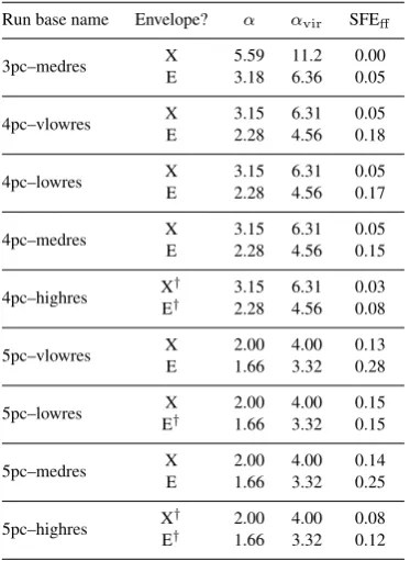
αand αvir for all simulations in Table 2. The runs which ended
before1.38tffare given withSFEfffor the latest time available.
[image:7.595.311.539.114.296.2]8
W. E. Lucas et al.
Table 2.Star formation efficiency per free-fall time along with the ratio of kinetic plus thermal to gravitational energy,α, and the virial parameter,
αvir. The values given for SFEffwere calculated using Equation (4) with
t0= 0.29tffandt= 1.38tffand are the data shown in Figure 7; the runs
indicated with a dagger did not proceed that far, and so have values of SFEff
given for the latest time they each reached.
Run base name Envelope? α αvir SFEff
3pc–medres X 5.59 11.2 0.00
E 3.18 6.36 0.05
4pc–vlowres X 3.15 6.31 0.05
E 2.28 4.56 0.18
4pc–lowres X 3.15 6.31 0.05
E 2.28 4.56 0.17
4pc–medres X 3.15 6.31 0.05
E 2.28 4.56 0.15
4pc–highres X
† 3.15 6.31 0.03
E† 2.28 4.56 0.08
5pc–vlowres X 2.00 4.00 0.13
E 1.66 3.32 0.28
5pc–lowres X 2.00 4.00 0.15
E† 1.66 3.32 0.15
5pc–medres X 2.00 4.00 0.14
E 1.66 3.32 0.25
5pc–highres X
† 2.00 4.00 0.08
E† 1.66 3.32 0.12
the virial parameter. As noted in Section 2, the5 pccloud was the most bound. The cloud alone was set up to have twice as much kinetic as gravitational energy, and so is found withα = 2.00as the thermal energy in the cloud was negligible when compared to kinetic energy. While the envelope was warm and so provided a great amount of thermal energy, the extra mass provided even more gravitational energy, resulting in the overall effect of the envelope being increase theα. This was the case with all runs.
With the shift inαprovided by the envelope, it can be seen in Figure 7 that, with some scatter, a relation exists between bound-edness andSFEff. This is particularly seen with E3pc–medres and
the X4pc runs which lay nearly on top of one another despite there being a factor of2.37difference in star forming cloud mass. X3pc– medres formed no stars and thus hadSFEff= 0. If one does form
a relation between the plotted quantities, then it may be thatSFEff
would go to zero for all values ofαabove perhaps four or five. To demonstrably show this would however require more simulations to fill this region.
4.4 Removing the envelope at later times
It is apparent that removing the envelope early on led to very dif-ferent star formation efficiencies. We decided to run an extra set of simulations derived from E4pc–medres in which the envelope was removed at several times before and after1tff, in an attempt
[image:8.595.68.255.173.429.2]to determine if there might be a critical point beyond which the re-moval no longer affected the SFE. The SFE is plotted against time for these simulations in Figure 8, which shows the original E4pc– medres simulation and others in which the envelope was removed at0.23(the original X4pc–medres),0.50,1.00,1.20and1.50tff.
Figure 8.Star formation efficiency of E4pc–medres and all derivative sim-ulations in which the envelope was removed at times later than0.23tff(the
original). Whether it took place before or after star formation had com-menced, the loss of the envelope always caused a drop in the SFE. Those clouds which lost their envelopes afterwards typically followed E4pc– medres for a short while before peeling away.
Star formation in E4pc–medres commenced at0.93tff.
Exam-ination of Figure 8 shows that the two simulations in which the envelope was removed before the first free fall time began forming stars only after that time. The simulations in which the envelope was removed from1.00tff onwards generally followed the E4pc–
medres curve for a short period of at most≈0.2tffafter the split
and then fell away after a brief period during which the cloud re-acted to the sudden loss of the envelope. This was not immediate: the gradients of the SFE in ‘late loss’ (>1.00tff) runs began high,
and slowly tended down over time towards values more closely re-sembling the gradients of the two ‘early loss’ (<1.00tff) runs. This
can in particular be seen for the two longest running simulations, those which lost their envelopes at0.50tffand1.50tff. It is possible
however that the downturn in the SFE as it approached0.7in the latter run actually occurred due to star forming material becoming more scarce.
Figure 8 makes it clear that a removal of the envelope in-evitably led to a reduction in the SFE, though a later removal brings it closer to that of the simulation which retained it. Thus no critical point for its effect would appear to exist, at least within the simula-tion runtimes achieved.
5 CONCLUSIONS
Star formation principally occurs in the cold and dense gas of giant molecular clouds. Yet these clouds will themselves be enshrouded with a warm atomic envelope, which can help to bind the cloud and thus keep it contained. It is possible however that feedback from nearby massive stars, whether in the form of ionisation, winds or supernovae, could blow away the envelope. As the envelope alters the cloud’s boundedness, we asked how its loss would change the star formation efficiency of the remaining dense molecular cloud.
clouds would have been unbound withα, the ratio of the kinetic plus thermal to gravitational energy, of5.59,3.15and2.00 respec-tively. The clouds were not evolved in isolation however, but rather they were placed within a warm envelope which provided a con-fining pressure boundary. The envelopes had a density a factor of ten lower, extending outwards in all cases to10 pc. With their pres-ence the values ofαwere lowered to3.18,2.28and1.66, again respectively with the3,4and5 pcclouds.
These simulations were evolved through to the point where stars could form, numerically represented by sink particles. How-ever, a parallel simulation was created from each of the originals after0.25tcrossof evolution. In these runs, the warm envelope was
instantaneously removed to leave only the cold central cloud. This was our first order approximation to the envelope’s removal by feedback.
We found for all three clouds that the removal of the envelope led to drastically lower levels of structure forming within the cloud while the external layers expanded. This naturally also caused the average densities to fall. As such it became harder for gas to be-come self gravitating and the levels of star formation fell.
The star formation efficiencies (SFEs) were calculated as a function of time. For all pairs of simulations (with and without the envelope), those which retained the envelope showed higher levels of star formation. At a fiducial time of1.38tff, the4and5 pcclouds
retaining the envelope showed SFEs higher by factors of 1.7 to 2.7 compared to the runs in which it was lost. The4 pcsimulations ran until a much later time and by≈1.8tff the discrepancy was even
higher with SFEs of≈ 0.5falling to≈0.15with the loss of the envelope.
The3 pccloud was the most unbound. At the same time of
1.38tff, it had an SFE of 5.67×10⁻² when the envelope was
present. In its counterpart which lost the envelope, no star forma-tion whatsoever took place.
Considering the star formation efficiencies per free-fall time (SFEff) and plotting these againstαshows the simulations to be
nearly a full sequence, with the3 pccloud with an envelope falling on almost the same point as the4 pccloud lacking an envelope, despite the larger cloud having2.37times the mass of the smaller.
We also ran a set of simulations derived from the4 pccloud in which the envelope was removed at later times. Even when it was lost as late as1.50tff, the SFE fell away to a slope resembling those
simulations which had lost the envelope at an earlier stage. In the runs in which the envelope was removed after star formation had begun, the SFE only responded to the loss after a short period of time of at most≈0.2tff.
A more realistic form of feedback may have brought about less extreme changes in the SFE than those reported here. For example, the envelope could have been lost only partially across some small solid angle, leading perhaps to the cloud’s expansion through the new opening as a cold outflow. Or, the envelope could have been lost slowly rather than removed instantaneously. However, the end state would have still resembled one of the simulations in which the envelope was removed at a later time. This implies that even then a drop in the SFE would be inevitable.
ACKNOWLEDGEMENTS
The authors thank Paul Clark for his contribution towards the orig-inal concept of this paper and the anonymous referee for their helpful comments. Our column density plots were produced us-ing Daniel Price’s SPLASH software (Price 2007). The authors
gratefully acknowledge support from the ECOGAL project, grant agreement 291227, funded by the European Research Council under ERC-2011-ADG. This work used the compute resources of the St Andrews MHD Cluster. This work used the DiRAC Complexity system, operated by the University of Leicester IT Services, which forms part of the STFC DiRAC HPC Facility (www.dirac.ac.uk). This equipment is funded by BIS National E-Infrastructure capital grant ST/K000373/1 and STFC DiRAC Op-erations grant ST/K0003259/1. DiRAC is part of the National E-Infrastructure.
REFERENCES
Abgrall H., Le Bourlot J., Pineau des Forˆets G., Roueff E., Flower D. R., Heck L., 1992, A&A, 253, 525
Ballesteros-Paredes J., 2006, MNRAS, 372, 443
Bate M. R., Bonnell I. A., Price N. M., 1995, MNRAS, 227, 362 Benz W., 1990, in Buchler R. J., ed., Proceedings of the NATO
Advanced Research Workshop on The Numerical Modelling of Nonlinear Stellar Pulsations: Problems and Prospects, Kluwer Academic Publishers, Dordrecht, p. 269
Bertoldi F., McKee C. F., 1992, ApJ, 395, 140
Bolatto A. D., Leroy A. K., Rosolowsky E., Walter F., Blitz L., 2008, ApJ, 686, 948
Bonnell I. A., Bate M. R., Vine S.G., 2003, MNRAS, 343, 413 Bonnell I. A., Larson R. B., Zinnecker H., in Reipurth B., Jewitt
D., Keil K., eds, Protostars and Planets V, University of Arizona Press, Tucson, p. 149
Bonnell I. A., Smith R. J., Clark P. C., Bate M. R., 2011, MNRAS, 410, 2339
Boss A. P., Bodenheimer P., 1979, ApJ, 234, 289
Clark P. C., Bonnell I. A., Klessen R. K., 2008, MNRAS, 386, 3 Dale J. E., Bonnell I. A., Whitworth A. P., 2007, MNRAS, 375,
1291
Dale J. E., Ngoumou J., Ercolano B., Bonnell I. A., 2014, MN-RAS, 442, 694
Dobbs C. L., Bonnell I. A., Clark P. C., 2005, MNRAS, 360, 2 Dobbs C. L., Burkert A., Pringle J. E., 2011, MNRAS, 413, 2935 Dobbs C. L. et al., 2014, in Beuther H. et al., eds, Protostars and
Planets VI, University of Arizona Press, Tucson, p. 3 Elmegreen B. G., Lada C. J., 1977, ApJ, 214, 725 Evans N. J. II, 1999, ARA&A, 37, 311
Evans N. J. II et al., 2009, ApJS, 181, 321 Federrath C., 2013, MNRAS, 436, 3167 Goldsmith P. F., Li D., 2005, ApJ, 622, 938
Heiderman A. Evans N. J. II, Allen L. E., Huard T., Heyer M., 2010, ApJ, 723, 1019
Heyer M. H., Brunt C. M., 2004, ApJ, 615, L45
Heyer M., Krawczyk C., Duval J., Jackson J. M., 2009, ApJ, 699, 1092
Heyer M., Gutermuth R., Urquhart J. S., Csengeri T., Wienen M., Leurini S., Menten K., Wyrowski F., 2016, A&A, 588, A29 Kennicutt R. C., Evans N. J. II, 2012, ARA&A, 50, 531 Krumholz M. R., Tan J. C., 2007, ApJ, 654, 304
Krumholz M. R., Dekel A., McKee C. F., 2012, ApJ, 745, 69 Krumholz M. R., Phys. Rep., 539, 49
Lada C. J., Lada E. A., 2003, ARA&A, 41, 57 Larson R. B., 1981, MNRAS, 194, 809 Larson R. B., 2005, MNRAS, 359, 211
10
W. E. Lucas et al.
Louvet F., et al., 2014, A&A, 570, 15
Mac Low M.-M., Klessen R. S., 2004, Rev. Mod. Phys., 76, 125 McKee C. F., Zweibel E. G., 1992, ApJ, 399, 551
MacLachlan J. M., Bonnell I. A., Wood K., Dale J. E., 2015, A&A, 573, 112
Monaghan J.J., 1992, ARA&A, 30, 543 Padoan P., Nordlund ˚A., 2011. ApJ, 730, 40 Parmentier G., Pfalzner S., 2013, A&A, 549, A132 Price D. J., 2007, PASA, 24, 159
Price D. J., Bate M. R., 2009, MNRAS, 398, 33 Price D.J., Monaghan J.J., 2004, MNRAS, 348, 139 Price D. J., Monaghan J. J., 2007, MNRAS, 374, 1347
Rosolowsky E., Engargiola G., Plambeck R., Blitz L., 2003, ApJ, 599, 258
Salim D. M., Federrath C., Kewley L. J., 2015, ApJ, 806, L36 Shu F. H., Adams F. C., Lizano S., 1987, ARA&A, 25, 23 Tohline J. E., 1980, ApJ, 235, 866