Generation of virtual asphalt mixture porosity for computational modelling

Generation of virtual asphalt mixture porosity for

computational modelling

A. Chiarelli∗_{, A.R. Dawson, A. Garc´ıa}

Nottingham Transportation Engineering Centre (NTEC), Faculty of Engineering, The University of Nottingham, University Park, Nottingham, NG7 2RD

Abstract

A new algorithm is proposed for the computational generation of realistic

as-phalt mixture porosity for computational simulations. The algorithm starts by

generating in a 2D domain a number of randomly positioned circular or

ellip-tical elements that are meant to represent virtual asphalt aggregate particles.

These elements are then grown by mimicking the biological mechanism called

contact inhibition until a target air voids content (AVC), chosen by the user, is

met. In addition, multiple 2D domains can be converted to 3D and combined

to generate a multi-layered realistic representation of the porosity present in

asphalt mixtures. In this paper, the working mechanism of the algorithm is

described and its efficiency is assessed. Moreover, the validity of the results is

discussed, and virtual domains, in both 2 and 3 dimensions, are compared with

real CT scans in order to show the efficacy of this approach. It was found that

the virtual representations of the asphalt mixture porosity show realistic

char-acteristics in terms of air voids content and that the air voids size distribution

is consistent with that of real specimens.

Keywords: asphalt, air voids content, packing, porosity

∗_{Corresponding author}

1. Introduction

Since the properties of asphalt pavements depend on the characteristics of

the particles they are made of, the importance of computational particulate

models that can describe them is undeniable. In particular, it is interesting to

focus on the role of porosity in asphalt pavements, as it influences the strength of 5

the material and its Young’s modulus [1]. Moreover, in [2], Chen et al. describe

the relationship between porosity and fluid flow, showing that also permeability

is a function of porosity.

In the literature many examples of computational particulate models can be

found, as reported in [3]. The options for the generation of asphalt domains 10

range from simple solutions based on 2D circumferences, to more complex

mod-els that imply the use of 3D rotated ellipsoids: the 2D option is clearly the

less realistic, while the 3D one requires more powerful computers to be run,

thus, the choice between them depends on the final use of the simulations. The

existing methods used to generate asphalt models from a particles assemblage 15

usually rely on physical principles, such as inter-particle friction, contact forces,

compaction energy, or drop and roll mechanisms [3, 4]. Moreover, models based

on statistical principles such as Monte Carlo methods can also be used [4].

The creation of specimens using these criteria is complex and requires a clear

understanding of the physics behind the processes that are used. For this reason, 20

it is complicated for users to understand clearly the working mechanisms that

power such methods, even if their results are reportedly realistic and provide

reliable tools for simulations.

The first issue in developing an asphalt assemblage is to select and position the

aggregate particles. The problem of generating packed particles in a finite or 25

infinite domain is also of great interest in the fields of physics and mathematics,

where it is related to fractal structures [5, 6, 7]. As reported in [8], Apollonian

Packing (AP) is the oldest known way to tackle the problem of packing particles

in space. The method consists in positioning a new particle (a disk in this case)

it touches all of them. This procedure is repeated many times in order to fill

all the voids created by the addition of new particles. Apollonian Packing

even-tually leads to a very dense system with the number of particles approaching

infinity, however it does not generate a randomized distribution of particles. As

shown in [8], an alternate system was developed to implement a Randomized 35

version of Apollonian Packing (RAP), but also in this case only one new particle

is placed each time. This model was generalized to an even greater extent in

the ABK model developed by Brilliantov, Krapivsky and Andrienko, where the

growth process is called “touch-and-stop model of growth” [9, 10].

Another method [7] generates a randomized distribution of packed particles in a 40

volume, but its aim is to simulate the motion of tectonic plates and the

appear-ance of seismic gaps, thus the particles are meant to organize themselves in a

system composed of bearings. The structure of the bearings makes it impossible

to obtain a realistic organization of the particles for an asphalt sample, as the

model is based on the fact that a particle must touch a number of other particles 45

(depending on the geometry, 2D or 3D) to be accepted [7], thus, no porous

chan-nel is allowed from and end of a 2D section of the domain to another, whereas

asphalt usually exhibits pore connectivity. Perhaps this limitation could be

overcome by the removal or particles from the domain; this, however, would

completely change the aim of the model. 50

2. Aims

The objective of this paper is to describe the development of a packing

method used to generate asphalt samples for the analysis of the porous space.

The method described in this paper is based on purely geometric concepts,

with-out the need of an extensive knowledge of particulate assemblage modeling. 55

The algorithm is able to create 2D and 3D domains, in order to allow different

kinds of computational analyses. The software developed in the present paper

follows the general idea of “touch-and-stop model of growth” [9]. An approach

slab with a structure that can be compared to real asphalt samples. The ran-60

domization of the parameters of interest enables the creation of a wide range of

possible configurations different from one another.

3. Development of the packing algorithm

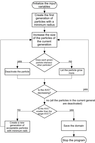
Default mode: 2D packing of circles. In Fig. 1 a flow chart of the algorithm is 65

shown.

The first step in the algorithm is the initialization of the operating variables,

which are the size of the domain, the number of centres for the first generation

of nucleating particles, the maximum size of the particles, and the target air

voids content (AVC). This last parameter is very important for the algorithm, 70

as it is the target to which it iteratively attempts to converge. Let us point

out that a difference exists between the real air voids content and the virtually

generated one. The assemblage of particles generated by the algorithm in two

dimensions does not include the bitumen mastic that fills much of the voids

between the aggregate particles in real asphalt. Thus, the value of AVC that is 75

obtained computationally (from now onAV C∗_{) should be reduced by a factor}

that takes into account the presence of the binder and the smallest stones,

that are smaller in size than the minimum particle diameter permitted in the

numerical procedure just described. This factor was chosen as 19% (7% binder

+ 12% filler, [11]), thus, 80

AV C[%] =AV C∗[%]−19% (1)

whereAV C∗_{is the air voids content generated by the software and AVC is the}

real value. As a result, at a computed AV C∗ _{equal to 25%, the real AVC is}

6%. Moreover, let us add that the value of the AVC that is calculated by the

algorithm is actually a measure of the 2D void area, thus, it does not correspond

to the 3D measure of the void volume. 85

Initialize the input variables

Create the first generation of particles with a minimum radius

Does each grown particle intersect other particles?

Increase the size of the particles of

the current generation

Deactivate the particle Let the particle grow more

Is the AVC* decreasing?

no yes

yes

Create a new generation of acceptable particles

with minimum radii

Is the AVC* smaller than the

target AVC*?

no (all the particles in the current generation are deactivated)

no

Save the domain yes

Stop the program

which are then turned into circumferences with a small radius. These

circumfer-ences are then grown according to the parametric equation of a circumference.

The circles are grown one by one and the algorithm checks if any intersection

between the growing particle and other particles takes place. If the growing 90

circle intersects other particles, it is deactivated and its radius is restored to

its previous value, while if there is no intersection the algorithm moves on to

another particle and repeats the same procedure.

At some point all the circles will be deactivated once they have all reached their

maximum allowed expansion (because they reached a maximum fixed radius or 95

because there is no more space available for their growth): this corresponds to

a value ofAV C∗_{, which is the parameter used to end the current growth loop.}

TheAV C∗ _{keeps decreasing while the particles are growing, and it stops}

de-creasing when they are all deactivated. At this point, in order to reach a lower

AV C∗_{, new particles are needed. Since one of the aims is to guarantee the}

100

randomization of the particle distribution, new centres for the new particles are

selected in random positions. Of course, many centres will not be in acceptable

positions, as they may fall on other particles or be too close to their edges to

allow a step of growth. These particles are discarded and not included in the

list of particles used for the growth steps that will follow. The new centres go 105

through the same procedure described before, until they are all deactivated and

a new generation of centres needs to be generated. After each generation, the

currentAV C∗ _{must be checked to see if it is less than the target AV C}∗_{. If it}

is, the procedure is stopped and the generated domain of particles is saved.

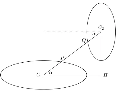
2D packing of ellipses. The generation of ellipses requires a further analysis due

to the fact that they have axes with different lengths, thus, their geometry can

not be so simply described. To begin with, note that two ways are available to

generate ellipses: the particles can be generated either with their axes parallel

to the axes of the coordinate system or with randomly rotated axes.

para-C1

C2

H α

α

P

Q

Figure 2: Geometric configuration for growing ellipses.

metric equation

x=a·cos(ω) +cx (2a)

y=b·sin(ω) +cy (2b)

where a and b are the major and minor radii of the ellipse, the centre of the particle is C = (cx, cy), and ω is a variable ranging from 0 to 2π. Only the length of the radii and the position of the centres need to be generated. The

initial length of the radii can be generated in any chosen way. For example,

one may use a randomized length for each radius, a normal distribution with a

chosen standard deviation, or fixed values. Another alternative is to determine

randomly one of the radii and calculate the length of the other one based on a

fixeda/bratio.

After this step, the procedure that is followed to increase the size of the ellipses

is similar to the one used for circles, with the only difference being the way that

geometric parameters of interest are computed as:

α=tan−1[|cy1−cy2|/|cx1−cx2|] (3a)

C1P=

p

(a1·cos(α))2+ (b1·sin(α))2 (3b)

C2Q=

p

(a2·cos(α))2+ (b2·sin(α))2 (3c)

d=

q

(cx1−cx2)2+ (cy1−cy2)2 (3d)

wheredis the distance between the centres and needs to be greater or equal to

C1P+C2Q. Every other part in the algorithm follows the mechanism described

in the case with circles.

In the case of rotated ellipses, everything becomes more complex, starting with

the equations that are used to describe the geometry of the particles:

x=a·cos(ω)·cos(θ)−b·sin(ω)·sin(θ) +cx (4a)

y=a·cos(ω)·sin(θ) +b·sin(ω)·cos(θ) +cy (4b) where θ is the rotation angle with respect to the horizontal direction. The 110

rotation angle is generated with a normal distribution centred on 0 and with an

appropriate standard deviation. As in the previous case with ellipses, the initial

length of the radii is determined by the user.

If rotated ellipses are used a problem arises in the computation of their

relative distance, because the geometric condition shown in Eq. 3d does not work 115

anymore. The reason for this is the fact that the geometric distance is not able to

take into account effectively some relative positions between the particles, thus,

allowing the generation of intersections. This problem is solved by detecting

directly the intersections between growing particles using a MATLABR _function that determines if a point or set of points lies inside a curve.

120

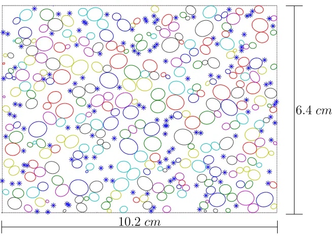
An example of the creation of a domain of rotated ellipses is shown in Fig. 3,

where a generation of new randomly positioned centres (represented by stars)

is being placed.

The method for the computation of the real AVC from the virtualAV C∗ _{is the}

0 0.02 0.04 0.06 0.08 0.1 0

0.01 0.02 0.03 0.04 0.05 0.06

Generation of new centers

Width [m]

Height [m]

10.2

cm

6.4

cm

Figure 3: Generation of new centres in the case of rotated ellipses.

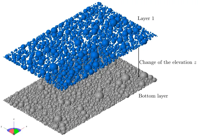
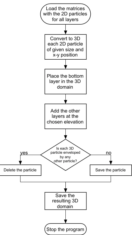
Generation of 3D pseudo asphalt mixtures. The algorithm is able to convert to

3D the domains generated in the 2D mode in the cases of circles and ellipses

with axes parallel to the main axes. This allows the creation of single layers

made of spheres or ellipsoids, where the position of the particles in each 3D

layer is determined by theirxandycoordinates in the original 2D plane. In the 130

case of ellipsoids, the out-of-plane dimension can be randomized about a mean

value with any desired standard deviation or it could be set equal to the major

or minor radius of the ellipse.

With a number of 3D layers it is possible to generate a slab made of previously

generated domains laid one on top of another. In order to do this, a first 3D 135

layer is chosen as the bottom of the slab being generated, then new layers are

positioned on top of it.

Each additional 3D layer is placed above the bottom layer at an elevationz, which is chosen by the user. A graphical representation of the process is shown

Change of the elevationz Layer 1

Bottom layer

Figure 4: Procedure to generate 3D multi-layered samples with 3D layers converted from 2D

packed domains.

different characteristics in terms of air voids content, as it influences how close

the 3D layers are placed from one another, thus, it determines how much void

space is left between them. So long as the layers are formed from non-identical

applications of the 2D algorithm, there will not be any repeating pattern that

could lead to undesirable shapes of the 3D voids. The flowchart of this procedure 145

is shown in Fig. 5.

Finally, let us add that the AVC is also controlled by choosing the 2D domains

that are converted to 3D and then combined, since the maximum 2D size of the

particles (either diameter of the circles or longer radius of the ellipses) highly

influences how they are going to intersect in the 3D multi-layered layout. 150

4. Implementation of the packing method

Initiation parameters. Initial values of many of the parameters are needed to

Load the matrices with the 2D particles

for all layers

Convert to 3D each 2D particle of given size and

x-y position

Is each 3D particle enveloped

by any other particle?

Delete the particle Save the particle

no yes

Save the resulting 3D

domain

Stop the program Place the bottom layer in the 3D

domain

Add the other layers at the chosen elevation

Figure 5: Flowchart of the algorithm for generating 3D slabs.

fixed are the height and width of the domain: as an example, the size of a cross

section of a cylindrical asphalt specimen is used, thus having a domain with a 155

height of 102mm and a width of 64mm (4x2.5in). A starting population of 500 particles and a maximum diameter of 35mm are used in the simulations shown in this paper.

1E−4m. In the case of ellipses, both radii are generated as random numbers 160

smaller than 1E−4m, then the longest between them is picked and the other one is obtained by multiplied the longest radius by an a/b ratio fixed as 0.7. This method allows the particles to have a shape similar to that of real stones

and ensures the creation of a randomized distribution of ellipses having their

longest radius oriented in the horizontal or vertical direction. In the case of 165

rotated ellipses, the ratio between the radii is also used, but applied directly to

the randomized size of one of the axes, i.e., one axis is generated as a random

number smaller than 1E−4 m and the other one is defined as the product between the random value and 0.7. This is done because in the case of ellipses with axes parallel to the reference axes the comparison between the values of 170

aand b is meant to generate “horizontal” or “vertical” particles, while in this case the randomized rotation angle serves the same purpose in a more general

way. The value of 1E−4mas the minimum size of the particles is used because everything smaller that that is likely to be part of the mastic in an asphalt

mixture. 175

In the algorithm for rotated ellipses, the standard deviation for the rotation

angle is fixed asπ/16 to take into account the fact that after compaction the stones are usually oriented along the x-axis (horizontal axis).

Depending on the computational resources (CPU and RAM), all these values

can be easily changed by the user to generate domains of any size and with 180

different characteristics.

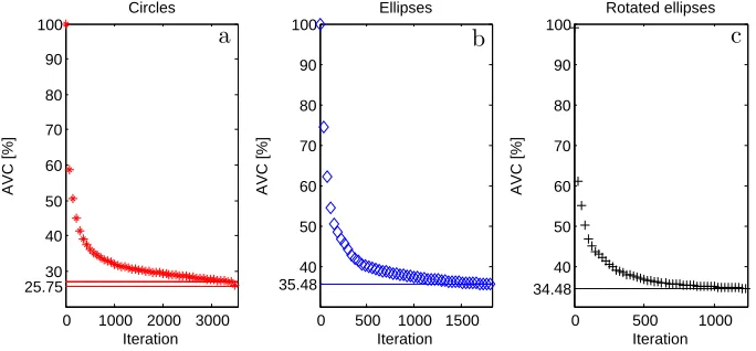
Convergence and computational time. As shown in Fig. 6, the algorithm runs

quickly in the first iterations, while it starts slowing down as it approaches

lower values ofAV C∗_{. Dodds et Al. [12] addressed a somewhat similar}

pack-ing problem, although uspack-ing a very different assembly method, and they also 185

experienced this slowing as void space becomes increasingly filled. Moreover,

not only the number of available voids decreases, but also their size becomes

increasingly smaller. For this reason, as convergence is approached the collision

0 1000 2000 3000 25.7530 40 50 60 70 80 90 100 Iteration AVC [%] Circles

0 500 1000 1500 35.48 40 50 60 70 80 90 100 Iteration AVC [%] Ellipses

0 500 1000

34.48 40 50 60 70 80 90 100 Iteration AVC [%] Rotated ellipses

a

b

c

Figure 6: AVC versus time for the cases under investigation.

placed far from one another and between already deactivated (not growing) 190

particles. Eventually there will come a point when the remaining voids between

the circles or ellipses cannot be filled with a circle or an ellipse of fixed

min-imum radius. Thus, a limit for the minmin-imum AV C∗ _{exists. Nevertheless, as}

this limit is approached, disproportionate computational time will be spent by

the algorithm in searching for new possible centres when the empty space is 195

very low and scattered. In order to allow the use of this method for practical

purposes, a convergence condition acting as a limit for the execution of the

al-gorithm was chosen. It was first attempted to set as a convergence condition a

relative difference in theAV C∗ _{of 2.5E−5 for two successive iterations.}

How-ever, the only algorithm that was able to achieve this goal in 2hwas the one 200

with circles, while the models with ellipses were stopped when they exceeded

the maximum allowed computational time time. This happened because for the

ellipses stricter conditions are applied for the acceptance of new centres, thus,

less space is filled at every iteration. For this reason, the relative variation of the

AV C∗ _{for two successive steps is smaller and cannot meet the required}

condi-205

tion. Therefore, the limiting condition for ellipses was adapted to the evolution

for the simulation with circles, 35.5% for the simulation with ellipses, and 34.5%

for the simulation with randomly rotated ellipses. The difference between the 210

two models with ellipses is related to the different ways the shapes occupy space

and to the different conditions that are applied for the acceptance of new

par-ticles (Euclidean distance vs. MATLABR _function).

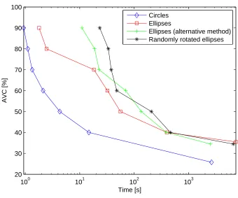
Furthermore, the model with rotated ellipses can be run with a rotation angle

set equal to zero so as to compare the generation of ellipses in the two ways. As 215

shown in Fig. 7, the use of the model for randomly rotated ellipses to generate

ellipses with no rotation provides slower void filling than does the simple ellipse

generation method down to 40% AV C∗_{, but past this point the randomly}

ro-tated ellipse generation algorithm is clearly more effective. The numbers shown

in Fig. 7 are only an example and were obtained as mean values for 100 simula-220

tions of each type. However, since the generation of points is randomized with

a uniform function, the computational time is always similar.

Domain tracking. Once the model approaches very low values ofAV C∗_{, and the}

generation of new particles in random positions has become extremely inefficient,

then the randomness of the distribution of particles is already guaranteed. At 225

this stage further reduction of the AV C∗ _{can be achieved by simply filling}

the voids with new particles without the use of a random generator. For this

reason, a domain tracker was implemented. The tracking algorithm starts when

the AV C∗ _{reaches 27%, which had been identified as the minimum practical} AV C∗_{for the algorithm generating circles. The line above the minimumAV C}∗

230

in Fig. 6a corresponds to a value of 27% and indicates that the next iterations

are all performed by the domain tracking algorithm.

The domain tracker creates a grid of points over the generated domain, then

it checks if they fall into the empty space or inside any of the circles. If a

point of the grid is in the empty space and far enough from any other centre 235

to allow a stage of growth, it is accepted as a new centre, as shown in Fig.

8. When all the points in the grid are checked, their growth starts following

100 101 102 103 20

30 40 50 60 70 80 90 100

Computational time

Time [s]

AVC [%]

Circles Ellipses

Ellipses (alternative method) Randomly rotated ellipses

Figure 7: Computational time for the 2D packing models.

times with a shifted grid, thus, many voids can be filled. However, since the

domain tracker starts when the algorithm that generates circles has reached an 240

already smallAV C∗_{, it is clear that theAV C}∗_{cannot decrease very much more,}

since a large part of the domain is already filled. A more dense packing can be

achieved by simply increasing the resolution of the grid, which by default is set

as 1E−3 (this obviously affects the computational time). The value of 1E−3 was chosen because a denser grid could lead to a regular arrangement of very 245

tiny particles in the remaining pore space whereas a smaller number of larger,

and pseudo-randomly positioned infill particles is required.

Other features of the software. The developed software is able to perform a

range of activities based on the data of the generated domain. One feature is

0

0.02

0.04

0.06

0.08

0.1

0

0.01

0.02

0.03

0.04

0.05

0.06

Width [m]

Height [m]

10.2

cm

6.4

cm

Figure 8: Result of domain tracking in the domain.

the software works with stages of growth and does not stop after every radius

increase. For this reason, the removal of particles from the domain allows a

direct control of the AV C∗ _{by the user, thus, making it possible to obtain}

intermediate values of AV C∗_{. The removing algorithm is again based on the}

randomization of numbers, i.e., if the user chooses to remove 100 particles, they 255

will be picked randomly from the domain and removed.

5. Examples of outputs of the algorithm

In Fig. 9 a virtual cross section generated in 2D (dense domain made of

circles) is shown.

A number of domains of the kind shown in Fig. 9 can be combined in order to 260

obtain a 3D multi-layered model like the one in Fig. 10. For the analysis of the

3D samples a clarification is needed. The 3D domains are meant to represent all

0 0.01 0.02 0.03 0.04 0.05 0.06 0.07 0.08 0.09 0.1 0

0.01 0.02 0.03 0.04 0.05 0.06

Final Air Void Content:25.7588

10.2

cm

6.4

cm

Figure 9: 2D virtual dense asphalt domain (circles), standard size in the software.

and intersect, thus, leaving empty volumes between them: for this reason, the

empty volumes are considered as the air voids, while everything else is part of 265

the asphalt mixture. In fact, the 2D and 3D domains generated here have a

completely different purpose: the bi-dimensional domain allows an analysis of

the components of the mixture, while the 3D model is focused on the generation

of voids rather than on the study of the surrounding material.

The 3D model shown in Fig. 10 was generated by trial and error in order to 270

reach a satisfactory result, as further studies are necessary to automate the

procedure that links the 2D air voids content to the corresponding 3D value.

Moreover, the 3D model needs to be repaired after its generation, because the

intersection of the particles results in a self-intersecting surface mesh. Finally,

let us point out that the extremes of the domain on axisy have to be excluded 275

from the analysis, as they have a very high air void content and possibly an

Figure 10: 3D meshed surface of a virtual slab of asphalt.

Mathematical background. Even if the aim of this software is to generate

do-mains for more practical applications, it is very interesting to briefly analyze the

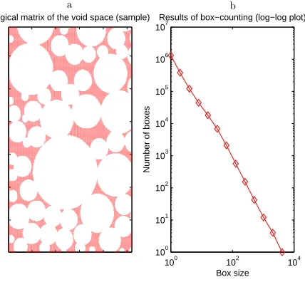
domain from a mathematical viewpoint. The theoretical analyses carried out in 280

[8], [12], and [9] led to the calculation of the fractal dimension of a sample

gener-ated domain. The analysis was performed considering the Minkowski-Bouligand

dimension (box-counting dimension) and its results are shown in Fig. 11 for the

domain made of circles shown in Fig. 9. In order to perform this kind of

analysis, a black and white high resolution image of a dense domain (∼25.75% 285

AV C∗_{) was printed and loaded in MATLAB}R_{, then a logical (binary) matrix} was generated and used to calculate the fractal dimension. Note that in Fig.

11a the circles seem to be overlapping: this effect is created by the 2D filling

functions in MATLABR _{and is also seen in Dodds et Al. [12].}

Fig. 11b reveals a log-log relationship between the number of boxes versus their 290

size according to a power law:

wherenbis the number of boxes and FD is the fractal dimension, calculated as the local slope of the curve shown. The value of the box-counting dimension is

constant in a given interval of box sizes (constant slope), thus, it is possible to

say that the domain shows a fractal behaviour for box sizes between 102 _and

295

103. The fractal dimension in the interval mentioned above is about 1.8 and

it is consistent with Liu et Al. [13], where values between 1.63 and 1.82 were

found.

The domain that was considered had the minimum value ofAV C∗_{it could reach}

after domain tracking (∼25.75% AV C∗_{). The analysis of samples with higher}

300

values ofAV C∗ _{was performed and it showed that the fractal properties were}

not present: the reason for this is that with highAV C∗_{(e.g., 80%) there is no}

repeating pattern and the domain has large voids.

Logical matrix of the void space (sample)

100 102 104 100

101 102 103 104 105 106 107

Box size

Number of boxes

Results of box−counting (log−log plot)

a b

Figure 11: Analysis of the fractal properties of the packed domain.

6. Comparison with real specimens

The purpose of the algorithm and its software implementation is to be a 305

tool for computational analyses. For this reason, a comparison with real CT

confirm the validity of the obtained results. Although direct 3D comparison

is conceivable, for reasons of practical convenience 2D CT scan images were

compared with 2D cross sections obtained from the generated 3D assemblage 310

described in this paper. Examples of such cross sections are shown in Fig. 12

and Fig. 13, which are the result of the analysis of the 3D domain displayed in

Fig. 10. The domain illustrated in Fig. 13 can be used for the analysis of the

air voids distribution as follows.

21-Sep-14 18:04:16

netfabb Snapshot

EVENTHICKER_fixed.fabbproject

asphalt mixture

air void Section A

Section B

Figure 12: Cross sections on the central axes of the 3D virtual slab shown in Fig. 10.

∼9.5cm

Figure 13: Section B elaborated from Fig. 12, (AV C=∼20.1%).

In order to perform the comparison between real and virtual samples, the 315

size of the air voids and their distribution were determined for a number of

cross sections. The CT scans of conventional and porous asphalt used for the

comparison are shown in Fig. 14. These binary images were obtained from

regular CT scans using a thresholding technique.

Sample 1

AV C= 14.97%

Sample 3

AV C= 12.90%

Sample 4

AV C= 7.59%

Sample 2

AV C= 22.28%

Figure 14: CT scans used for the comparison with the computationally generated asphalt

mixture porosity.

The outliers in the distribution of pores were excluded from each set of 320

values by eliminating the pores with an area with a statistical standard score

larger than 3. The standard score can be calculated by subtracting the mean

value of a set of data from each element in the set and by dividing the obtained

difference by the standard deviation of the data under analysis. The result

of this procedure is shown in Fig. 14, where the distribution of the air voids 325

size is represented as a dimensionless quantity on the x axis. In Fig. 15 it is possible to notice that the distribution of the size of the air voids in the

virtual specimens shows a realistic behaviour, being encompassed by the other

curves. It is interesting to note that certain sized voids are largely missing from

the computed assemblage, but that this phenomenon is shared by the scans of 330

genuine asphalt. A plot obtained from a single use of the 2D algorithm described

CT scan curves and, therefore, this suggests that the assembly of a 3D model

may not always be necessary where a 2D analysis of pore structure is required.

0 0.2 0.4 0.6 0.8 1

0 0.1 0.2 0.3 0.4 0.5 0.6 0.7 0.8 0.9 1

Size of void / Size of largest void

(i−0.5)/n

Virtual domain 2D Virtual domain 3D Real CT scan 1 Real CT scan 2 Real CT scan 3 Real CT scan 4

Figure 15: Comparison of the air voids distribution of the virtual samples cross sections with

real CT scans.

7. Applications

335

In the field of civil engineering, the algorithm could be used to perform

computational analyses of the thermal or mechanical properties of asphalt

spec-imens without the need of making CT scans, which require time and the proper

machinery. In addition, studies about the hydraulic conductivity could be

The major limitation of the algorithm developed is that at the present time

it is not able to stack autonomously the 3D planes of particles, therefore this

operation needs to be performed with a purposely generated script. Moreover,

since the algorithm generates particles, in order to analyse the void space

be-tween them the user has to elaborate further the 3D models that are created. 345

This could be avoided by shaping directly the pore structure, as done in other

studies [14, 15]. However, the theoretical concepts used in [14] and [15] are more

complex than those used in the algorithm developed here, which was studied to

simplify the approach to the computational generation of porous media.

Even if the algorithm described here was meant to be used to simulate asphalt 350

specimens, its results can be used for many other applications. The very general

approach used allows wide application, although its final purpose could

influ-ence strongly its setup and use.

For example, the model could represent particles that can only have a fixed

shape due to surface tension, as reported by Andrienko et Al. [10]. Another 355

application is obviously in crushed stone, grain, or bead and ball packing

prob-lems, where the most efficient way to organize items is investigated. Finally,

Brilliantov et Al. [9] state that pattern formation processes are very important

for a wide variety of natural phenomena (diffusion-limited aggregation,

den-dritic growth, dielectric breakdown, etc.), thus, this algorithm and its software 360

implementation could be useful for more theoretical applications linked to the

study of repeating structures.

8. Conclusions

In this study, a new method to generate virtual asphalt mixture porosity

was developed and an analysis of the results was performed. The following 365

conclusions can be drawn:

• The virtual samples generated with this method show realistic

character-istics in terms of air voids content and voids distribution, both in two and

• The comparison with real CT scans proved the validity of the approach, 370

although the generated domains are probably not suitable for microscopic

void analysis.

• The randomization of all the parameters of interest ensures the generation

of a virtually infinite number of different samples, thus, allowing the user

to perform various kinds of analyses on realistic asphalt mixture cross 375

sections without the need of CT scans.

• The algorithm is very flexible and domains of any size can be generated

easily and in a limited amount of time.

• An approach based on geometric criteria was proved to be effective even

if it is theoretically simpler than previous methods for the generation of 380

asphalt mixtures based on physical concepts.

• Since the algorithm is mainly based on geometry, the generation of asphalt

mixture porosity can be seen as a practical application of a more general

method that can be used for various purposes, ranging from mathematics

to engineering. 385

9. Acknowledgments

The authors thank the University of Nottingham for the financial support

provided for the Ph.D. of Andrea Chiarelli.

10. References

[1] M. P. Schpfer, S. Abe, C. Childs, J. J. Walsh, The impact of porosity and 390

crack density on the elasticity, strength and friction of cohesive granular

materials: Insights from dem modelling, International Journal of Rock

Me-chanics & Mining Sciences 46 (2009) 250–261. doi:10.1016/j.ijrmms.

[2] Y. Chen, C. Shen, P. Liu, Y. Huang, Role of pore structure on liquid flow 395

behaviors in porous media characterized by fractal geometry, Chemical

En-gineering and Processing 87 (2015) 75–80. doi:10.1016/j.ijrmms.2008.

03.009.

[3] M. Jiang, J. Konrad, S. Leroueil, An efficient technique for generating

homogeneous specimens for DEM studies, Computers and Geotechnics 30 400

(2003) 579–588. doi:10.1016/S0266-352X(03)00064-8.

[4] R. Isola, Packing of granular materials, Ph.D. thesis, The University of

Nottingham (2008).

[5] H. J. Herrmann, G. Mantica, D. Bessis, Space-filling bearings, Physical

review letters 65 (1990) 3223–3225. doi:10.1103/PhysRevLett.65.3223. 405

[6] G. Oron, H. J. Herrmann, Generalization of space-filling bearings to

arbi-trary loop size, Journal of Physics A: Mathematical and General 33 (2000)

1417–1422. doi:10.1088/0305-4470/33/7/310.

[7] R. M. Baram, H. J. Herrmann, Random bearings and their stability,

Physical Review Letters 95 (2005) 224303–1–224303–4. doi:10.1103/ 410

PhysRevLett.95.224303.

[8] G. W. Delaney, S. Hutzler, T. Aste, Relation between grain shape and

fractal properties in random apollonian packing with grain rotation,

Physical Review Letters 101 (2008) 120602–1–120602–4. doi:10.1103/

PhysRevLett.101.120602. 415

[9] N. V. Brilliantov, P. L. Krapivsky, Y. A. Andrienko, Random

space-filling-tiling: fractal properties and kinetics, Journal of Physics A: Mathematical

and General 27 (1994) L381. doi:10.1088/0305-4470/27/11/006.

[10] Y. A. Andrienko, N. V. Brilliantov, P. L. Krapivsky, Pattern formation by

growing droplets: The touch-and-stop model of growth, Journal of Statis-420

[11] J. Rebbechi, Stone Mastic Asphalt - Design & Application Guide,

Aus-tralian Asphalt Pavement Association (2000).

[12] P. S. Dodds, J. S. Weitz, Packing-limited growth, Physical Review E 65

(2002) 056108–1–056108–6. doi:10.1103/PhysRevE.65.056108. 425

[13] T. Liu, X. Zhang, Z. Li, Z. Chen, Research on the homogeneity of asphalt

pavement quality using x-ray computed tomography (ct) and fractal theory,

Construction and Building Materials 68 (2014) 592–593. doi:10.1016/j.

conbuildmat.2014.06.046.

[14] M. Siena, M. Riva, J. D. Hyman, C. L. Winter, A. Guadagnini, Relationship 430

between pore size and velocity probability distributions in stochastically

generated porous media, Physical Review E 89 (2014) 013018. doi:10.

1103/PhysRevE.89.013018.

[15] J. D. Hyman, P. K. Smolarkiewicz, C. L. Winter, Pedotransfer functions

for permeability: A computational study at pore scales, Water Resources 435