Computations in Stochastic Game Theory : large sets of rewards in games with communicating states and frequency dependent transition probabilities and stage payoffs

(1)

1

Faculty of Behavioural

Management & Social Sciences

M.Sc. Program: Industrial Engineering & Management

Specialization: Financial Engineering & Management

Master Thesis

Computations in Stochastic Game Theory

Large sets of rewards in games with communicating states

and frequency-dependent transition

probabilities and stage payoffs

Llea Nasira Samuel s1543261 April 28, 2017

(2)

Master Thesis, University of Twente.

Computations in Stochastic Game Theory. Large sets of rewards in games with commu-nicating states and frequency-dependent transition probabilities and stage payoffs.

This research project was performed under the supervision of dr. R. A. M. G. Joosten in partial fulfillment of the Master of Science degree in Industrial Engineering & Management.

Faulty of Behavioural Management & Social Sciences (BMS)

(3)

Page i

Acknowledgements

I am of the firm belief that in order to arrive at the stage of producing a Master thesis of a level that has resulted in the ability to publish new findings, had been due to the efforts of many more individuals than just the author of this thesis.

First and most obvious, Reinoud Joosten. Without him, I would still be floundering without an idea for a thesis project, much less the invaluable assistance he has provided during the project’s development. His unique viewpoint into stochastic game theory and ability to accurately explain the crossover from theoretic to computational has proven to be irreplaceable.

Also to Dr. Berend Roorda, whose insight saved my thesis from being a collection of tech-nical jargon instead of the easy-to-follow read-through most readers will experience in the coming pages.

Second, my family and close friends to whom I owe the mental fortitude that allows me to step confidently and happily from one day into the next.

Thirdly, the administration at the University of Twente, specifically, the International Office, Student Services and those overseeing us Industrial Engineering & Management M.Sc. students.

To anyone else I may have forgotten, you know who you are. Thank you.

(4)

Abstract

With the amount of conceptual literature on 2-person social dilemmas, this thesis takes the neces-sary step of creating an algorithm that is able to compute what has been modeled. That is: dynamic 2-state, 2-player, 2-action stochastic competitive games with allowances for frequency-dependent transition probabilities and frequency-dependent stage payoffs. To demonstrate its usage, I em-ploy a ‘Commons’-type social dilemma where 2 players compete over arenewable common-pool

resource. In this example, both the transition probabilities and stage payoffs possess frequency-dependencies that are linear. Note that adherence to such a limitation is not necessary for the stage payoffs, but may be for the transition probabilities.

Results in both the repeated game model and the two stochastic models are in line with results found in prior studies. That is, frequency-dependent stage payoffs cause a reduction in the value of the payoffs available as the reward set heads south-west inR2. More noteworthy, results in

the stochastic models with frequency-dependent stage payoffs show that frequency-dependent trans-ition probabilities have significantreduction effectson theprobabilityof obtaining a higher payoff

for either player. The reward sets in both situations increase in size by stretching toward the origin, compared to the frequency-independent stage payoffs reward sets. This increase is compensated in part through a narrowing of the set’s shape inR2space which results in smaller differences between

both players when one gains more than the other.

(5)

1. Introduction

Van Lange, Joireman, Parks and Van Dijk (2013) define social dilemmas as

...situations in which a non-cooperative course of action is (at times) tempting

for each individual in that it yields superior (often short-term) outcomes for self, and

if all pursue this non-cooperative course of action, all are (often in the longer-term)

worse off than if all had cooperated.

From such a definition, one can conclude that social dilemmas can be either momentary or dynamic. The dynamic element contains both short term and long term outcomes.

To better understand the significance of these differentiations, I will explain one of the most common examples of a social dilemma: The Prisoner’s Dilemma. In this scenario, two pris-oners must decide whether or not to rat each other out to the police in order to receive a reduced sentence handed down by the judicial system. More specifically, each prisoner (arbitrary labels ‘A’ and ‘B’) is aware that if A rats out B, A receives a reduced sentence for his (her) cooperation with the judicial system, while B receives the largest sentence possible. If both A and B rat each other out, reduced sentences are give to each. But such a reduction is trivial when compared to the time added on due to the other’s betrayal.

In game theoretic terms this reduced sentenced is called thepayoff and the choices of

whether to cooperate with the police or not are theactions. The prisoners (usually two, but can be

more) are calledplayers. The entire situation is referred to as agame.

(10)

Page 2 Chapter 1. Introduction

Because if one rats the other out, whilst the other does not, thedefectorgets a significantly reduced

sentence. But if they both defect, they both get harsh sentences. This pair of harsh sentences is the Nash equilibrium as they correspond to each player’s dominant action choice. However, there is also the option of their both remaining silent. This gives a smaller sentence to each which is not the dominant action, but it is still better than the Nash equilibrium. This idea is considered through

Pareto optimality. Hans Peters (2008) defines:

A pair of strategies is Pareto optimal if there is no other pair such that the

as-sociated payoffs are at least as good for both players and strictly better for at least

one player.

This makes the Nash equilibriumPareto inferior, and the choice of remaining silent isPareto su-perior.

When considering the time element, first assume that both prisoners cooperate and remain silent. If this is a finitely repeating game (say the situation happens 5 times), then on the fifth play, both players will feel inclined to rat the other out, as the situation will never again repeat itself thus incurring the wrath of the other. So for the fifth iteration, the dominant action is played. However, as both players suspect the other of this at the fourth repetition, they use this earlier opportunity to defect. This way of thinking can occur at every prior repetition till the first time the situation occurs, resulting in the outcome thatfor allrepetitions, prisoners ‘in cahoots’ will feel inclined to

betray the other.

Interestingly enough, this may not be the case if the game repeats infinitely. From the logic above, if the end point is never met, the prisoners have no option in which to rat the other out without incurring the punishment of the other in the subsequent repetition. Using the notation for repetitions ast= 1,2, . . ., we see that in some instances, the prisoners will rat each other out early

in the game: whentis close to 1. In other instances,tmay indeed be large, but the point at which

the cooperation between the two falls apart will eventually make prior outcomes insignificant. For example, if the point at which the prisoners decide to rat each other out is t0 = 1 mil, all the

cooperative outcomes prior tot0 are trivial when faced with the Nash equilibrium result for every tfromt0 to∞. Thus, long term considerations can prove an interesting means of studying social

dilemmas.

(11)

1.1 Game Theory in Social Dilemmas Page 3

Mirman (1980) and more recently by Joosten (2007): fishery wars. In fishery wars, there is a large renewable common-pool resource from which all the fishermen obtain their catch. This is an example of a ‘Commons’-type dilemma like that described by Hardin (1968). For fisheries,

the renewable common-pool resource is the oceans, seas and lakes. Short term gain here results from ‘fish as much as you want’ actions and can have a devastating effect on the long term possible payoffs because the resource is not given sufficient time to replenish.

1.1 Game Theory in Social Dilemmas

A unique perspective on these types of scenarios was developed by Brenner and Witt (2003) and by Joosten, Brenner and Witt (2003). By making adjustments torepeated games, they were able

to derive a method by which the past actions of the players influence the payoffs they can receive now. This puts a rather realistic slant to the social dilemma concept. Obviously, many situations in society tend to repeat themselves (these repetitions are calledstages), and the actions performed

by the players are most likely influenced by the number of times the situation has occurred in the past, and what the outcomes had been. Joostenet al.(2003) coined the name ‘frequency-dependent

(F D)-games’. This enhances the idea that it is thefrequency with which past stage payoffs have

been achieved that can affect the current stage payoff, as opposed to situations in which the current stage payoff is uninfluenced by what has happened in the past.

Later on, a new study added further realism to the study of social dilemmas: a stochastic game model by Joosten and Meijboom (2010). Stochastic games consider situations in which the possible payoffs available, changes. Each set of payoffs, and the actions through which they are achieved, is referred to as astate, making a stochastic game a multi-state game. The changing from

one state to another is dictated by a transition probability matrix.

Joosten and Meijboom (2010) developed their own algorithm which considered how frequency-dependent transition probabilities would affect games with frequency-independent stage payoffs. The algorithm placed particular emphasis on the effects produced in temporarily absorbing states. With no focus on absorbing states, my thesis examines communicating states only. Unlike absorbing states, communicating states are those in which the probability of leaving a particular state or of remaining in a particular state isnever zero at any timet(for more on communicating

(12)

Page 4 Chapter 1. Introduction

their model cost Joosten and Meijboom significant processing time especially in what I refer to as their ‘Type III’ model (see Table 1.1); a point that will be elaborated on in theConclusion, after my

algorithm has been explained.

Mahohoma (2014) considered stochastic games with frequency-independent transition

probabilities, yet the stage payoffsarefrequency-dependent. To avoid confusion, it seems

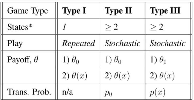
appro-priate to summarise previous research in this area in a table: Table 1.1.

Game Type Type I Type II Type III

States* 1 ≥2 ≥2

Play Repeated Stochastic Stochastic

Payoff,θ 1)θ0 1)θ0 1)θ0

2)θ(x) 2)θ(x) 2)θ(x)

Trans. Prob. n/a p0 p(x)

Table 1.1: A Table of Games.θ(x)andp(x)represent the dependency on the history of play of the payoff and transition probability respectively. Literature has been rigourous

enough to encompass 2+ player models. For simplicity in model-building, this thesis

is restricted to 2-player games.

There1_{, using my notation one can see that Joosten}_{et al.}_{(2003) did work in Type I [}_θ₍_x₎_]

games. Mahohoma’s work (2014) was in Type II [θ(x), p0] games, with Joosten and Meijboom

(2010) in Type III [θ0, p(x)] games. In this Master thesis I take the next step in model development:

Type III [θ(x), p(x)] games.

1.2 Thesis Aim and Paper Organisation

The aim of this thesis is to create a model that can commute multiple reward sets of a 2-player,

2-action, 2-state stochastic game with communicating states and frequency-dependent transition

probability and/or frequency-dependent stage payoffs. As a step-by-step approach is taken in the

1_{Note that this table is a work in progress. The initial understanding of what differentiated a repeated game from a}

(13)

1.2 Thesis Aim and Paper Organisation Page 5

algorithm’s development, a by-product of this aim will be the development of, not just one, but a set of Matlab©_{algorithms that encompasses all the computations and methodology noted in Table}

1.1.

(14)

(15)

2. Methodology

In a single-play competitive game, there is only one instance in which the players decide their action choices (an ‘action pair’ for a 2-player game like the one studied here). This single instance results

in a single payoff to each player. As stated in the introduction, a repeated game contains multiple instances called stageswhere the players choose their actions. These stages follow discrete time

step t = 1,2,· · · , T, with each stage having its own stage payoff. In this section I explain the

relationships among stage payoffs, rewards and reward sets, the frequency matrix and the transition probabilities in repeated and stochastic games, as generated by the algorithm.

2.1 Necessary Conditions

In order to employ the methodology employed in Joostenet al.(2003), there are a few requirements

that must be explained.

2.1.1 Jointly-Convergent Pure Strategies

On pure strategies. If at staget, a player’s action is chosen with 100% probability, it is called a

pureaction. A set of a player’s pure actions is apure strategy. That is, at every stage of the play, in

every state of the game, the player uses one of the available actions with probability 1.

(16)

Page 8 Chapter 2. Methodology

(see Fig. 2.1) is written as

Xt =



 xt₁ xt₂ xt₃ xt₄



 (2.1)

For example, for a game with 1000 repetitions having taken place, players choices have set the game play in the upper left element 100 times, the lower left elements 3 times, the upper right element for 850 times and 47 times in the lower right element is described by:

X1000 =

  100 1000 850 1000 3 1000 47 1000 

, (2.2)

so that for this game,

X1000 =





0.100 0.850

0.003 0.047



. (2.3)

The condition of Eq. (2.4) becomes obvious:

4

X

i=1

xt_i = 1 (2.4)

Thethere labels all the times the payoff corresponding to that position in the payoff matrix

was obtained up till timet. Additionally, thetsuperscript indicates that for every stage, there exists

a different value forxt

i. For example, if after only 100 iterations of the game just described,

X100 =





0.00 0.90

0.02 0.08



 (2.5)

then we see that X100 ₆₌ _X1000_{. In general} _Xt _{may not necessarily be equal to} _Xt+1_{. When a}

strategy is said toconverge, each of these four values converges to a certain four numbers for every

tin the long run (i.e., forT → ∞). Joostenet al. (2010) formalise this from the perspective of the

players’ strategies.

Ifπ represents the strategy used by player 1 (e.g. $\pi=$ action 1, action , 2 action 2, action

1, for a four stage game) andσrepresents the strategy used by player 2, we can say the following:

A strategy pair (π, σ) isjointly convergentif

∀>0∀i lim sup t→∞ Prπ,σ

(17)

2.2 Repeated Games Page 9

Prπ,σ represent the probability associated with the strategies of both players. ‘lim sup’ is the limit

superior with anyε >0. Eq. (2.6) allows for the following matrix definition:



 xt

1 xt2

xt

3 xt4





(T→∞)

−−−−→



 x1 x2

x3 x4



 (2.7)

whereP4

i=1xi = 1.

2.1.2 Long Run Average Reward

There are various ways of evaluating the scenario in which T → ∞ in repeated and stochastic games. A simple one would be to add up all the stage payoffs. Here, like in Joostenet al. (2003), I

use thelong run average reward:

ϑk(π, σ) = lim inf

T→∞ 1 T T X t=1

ϑk_t(π, σ) (2.8)

where(π, σ)represent the strategies of players andϑk

t(...)is the expected payoff at stagetto players

k = 1,2. ‘lim inf’ is the limit inferior. We use the ‘lim inf’ as the average need not exist.

2.2 Repeated Games

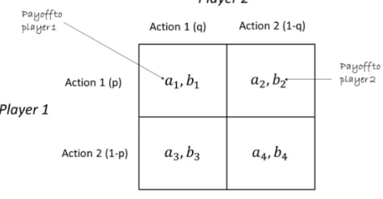
2.2.1 Payoff Matrix and Frequency-Dependent Rewards

The setup for a 2-player, 2-action repeated game is shown in Fig. 2.1. The payoff per stage of the

Figure 2.1: A Competitive Game

(18)

players at that stage. Theaverage reward until staget in a 2-player game with jointly converging

strategies is provided by a combination of the stage payoffs and the stage frequencies ofXt_when_t

is large:

θt[pl1, pl2] =xt1(a1, b1) +xt2(a2, b2) +xt3(a3, b3) +xt4(a4, b4)

=

4

X

i=1

xt_i·θi (2.9)

whereθi = (ai, bi)andplt1refers to the average payoff for Player 1. If we set limits ast →0, we get

Eq. 2.8 The superscript onθ means that aftertiterations, there is aset of rewardsthat the players

have obtained for that game. This reward set can be used to make areward spaceinR2.

In order to ensure that the code is functional, the algorithm is tested using

Θ =



 θ1 θ2

θ3 θ4



= 



16,16 14,28

28,14 24,24



 (2.10)

Like the Prisoner’s Dilemma, the lower right value is the Nash equilibrium. However, unlike the Prisoner’s Dilemma, this value is Pareto superior to (‘dominates’) the upper left value which is

now its Pareto inferior. The Pareto superior value represents ‘abuse’ of a hypothetical renewable common-pool resource. That is, the resource cannot sustain such a large number being removed consistently over time. On the other hand, the Pareto inferior value in the upper left of the matrix does allow for a renewability of the resource. In this manner, Eq. (2.10) models a ‘Commons’

dilemma. We can consider the Pareto inferior to be the long term ‘best for both’ (BB) payoff pair, and the Pareto superior to be the short term BB payoff pair.

2.2.2 Frequency-Dependent (F D) Payoffs

Obtaining any of these payoffs before current timet, affect the common-pool total. This aspect is

considered through afrequency-dependent function. F Dfunction, for short. Section 2 of Joosten

(2016) builds a methodology explaining how theF D is formulated. With theF D, the payoff is

seen as a fractional value of the reward in Eq. 2.9. Mainly,

Payoff =F D·θt[pl1, pl2] (2.11)

For the purposes of algorithm building, I use a simple linearly decreasing function of the form:

(19)

2.3 Stochastic Games Page 11

The absence ofx1 in the formula emphasises the idea that an ecologically-friendly

ap-proach to fishing should not affect the stock; γ4 > γ1 ∈ [0,1]because both players abusing the

resource simultaneously is more harmful to the fish stock than individual abuse. The restrictions onγ2andγ3are that

1. they are both non-negative, and 2. (γ2x2+γ3x3)< γ1−1

γ2 6= γ3 represent situations in which there is only one abuser who does more damage to the fish

stock than the other when the other is the lone abuser. For the Type I games produced here, let

F DI = 1−

1

4(x2+ 2x3)− 2x4

3 (2.13)

The subscript represents the game type to which theF Dfunction is applied.

2.3 Stochastic Games

Stochastic games contain multiple states (payoff matrices) and a transition probability matrix, that determines which of these states the play will move from stage (t) to stage (t+ 1). This makes a

repeated game a stochastic game with a transition probability of 1 that the stage (t+ 1) remains in

the current state.

2.3.1 Multiple States

As Table 1.1 showed, the Type II and Type III games studied here have at least two states each. Joosten and Meijboom (2010) refer to these asHighandLowstates. For this study, High

corres-ponds toS1- the situation in which renewability of the resource can occur; and Lowcorresponds

toS2 - the situation in which renewability of the resource is not given sufficient time to replenish

itself.

To test the algorithm, these values were used:

ΘS1 = 



16,16 14,28

28,14 24,24



 ΘS2 = 



4.0,4.0 3.5,7.0

7.0,3.5 6.0,6.0



 (2.14)

The repeated game mentioned earlier can be made by setting the probability of moving to S2 as

(20)

2.3.2 Transition Probability Matrix

The transition probability matrix determines with what probability the play will move from one state to another (or the same state) for the next stage. For a 2-state system, each matrix contains elements that read as:

(probability of moving toS1 att+ 1,probability of moving toS2att+ 1)

where both values sum to 1.

The numerical example used here is:

pS1

0 =





0.8,0.2 0.7,0.3

0.7,0.3 0.6,0.4

  p S2 0 =  

0.5,0.5 0.40,0.60

0.4,0.6 0.15,0.85



 (2.15)

where the subscript (0) represents a transition probability that is independent of the frequencies (non-FD).

For ease of use, the matrices are re-written as a single vector containing only the probab-ilities of transitioning toS1 att+ 1for the algorithm.

p0 =

h

0.8 0.7 0.7 0.6 0.5 0.4 0.4 0.15

i

(2.16)

2.3.3 Frequency-Dependent Stage Payoffs in Stochastic Games

Multiple-states means more xvalues are required. For a 2-state, 2-action, 2-player system where t→ ∞,

8

X

i=1

xt_i = 1 (2.17)

resulting in two matricesX∞₁ andX∞₂ , where the subscripts refer to the state which they represent.

As shown in Eq. (2.18), the frequency vector is an element of the 7-dimensional space∆7.

xt∈∆7 ={x∈_R8_|_x

i ≥0for alli= 1, . . . ,8and

8

X

i=1

xi = 1} (2.18)

For a 2-player game, this frequency point is projected onto a 2-D plane. This results in some interesting plots, as will be seen in the results.

TheF Dfunction corresponding to the example being described here should also include

these additionalx-terms. Again, I use a simple linear function, this time a version specific for Type

II and Type III games. Let:

(21)

2.4 Computing Type II and Type III Games Page 13

Along with the restrictions as stated for Eq. 2.12,x5is not present as it does not affect the resource,

andγ4 < γ8 andγ1 < γ5. This latter restriction is due to the fact that abuse in state 2 is worse than

abuse in state 1 because state 2 contains less of the resource than state 1.

For the algorithm, I employ the following example, based on Eq. 2.19:

F DII,III = 1−

1

4(x2+x3)−

x4

3 − 1

2(x6 +x7)− 2x8

3 (2.20)

2.4 Computing Type II and Type III Games

To recap, there are three types of games (I, II, III). The first contains a single matrix (state), the other two contain two matrices (in my example, but can contain more) of possible payoffs for 2 players who each have two action choices that can be played at timet. There is an average reward

corresponding to each pair of actions. Using anF D- function on the average reward at timet, one

can obtain the payoff specific to that time, given the history of playup totimet.

The next step: how to determine what the history of play was? That is, what are the elements of matrixX∞?

2.4.1 Random Sampling

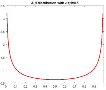
I obtain values for theX∞matrices via theβ-distribution. Aβ-distribution is a distribution which

contains all possible values of an unknown probability. As interesting things tend to happen with the smallest probability, it may prove most interesting to use the least likely probabilities (that is, those close to 0 and 1). Additionally, focusing on the least likely values, will provide a broad range of reward set values the quickest (faster than the uniform distribution). To do this, the variables for theβ-distribution are set to 1₂. This increases the likelihood of choosing values close to the edges

of the distribution (Fig. (2.2)). A distribution of this type is referred to as aU-shaped Distribution.

2.4.2 Random Sampling and the Transition Probability

A constraint to these randomly chosenxvalues is that they must fulfill theflow equation.

4

X

i=1

xi(1−pi) =

8

X

i=5

xipi (2.21)

whereirefers to the vector’s element number. If the flow equation holds, the system’s states can be

classified as communicating in the long run. Thus,P4

i=1xi(1−pi)6= 0and

P8

(22)

Figure 2.2: The U-shaped β-distribution is made

when bothαandβare set to one half.

results in either state 1 or state 2 (respectively) being an absorbing state.

In order to perform this calculation, usage of an intermediate vector y and a dummy

variable Q are required to obtain the necessary degree of freedom. The values that fit the Eq.

(2.21) are stored in the vectorx∗. ForS1:

yi =

xi

P4

j=1xj

i={1,2,3,4} (2.22)

and forS2

yi =

xi

P8

j=5xj

i={5,6,7,8} (2.23)

yis related tox∗via:

x∗ =hQy1 Qy2 Qy3 Qy4 (1−Q)y5 (1−Q)y6 (1−Q)y7 (1−Q)y8

i

(2.24)

Using Eq.s (2.23) and (2.22), Eq. (2.21) in terms ofygives

Q

4

X

i=1

yi(1−pi) = (1−Q)

8

X

i=5

yipi (2.25a)

Q=

P8

i=5yipi

P4

i=1yi(1−pi) +

P8

i=5yipi

(2.25b)

OnceQis determined (and by extension,1−Q), it is a simple matter of utilizing Eq. (2.24) once

(23)

This way, one can see that I move from the randomly (β-distribution) chosen values of

X∞ to an intermediate matrix y, to solving for Q, and finally obtaining the corrected X∞ matrix that transitions fromS1 toS2and back: x∗ =x(y, Q).

In the case (of 2+ states), Eq. (2.25b) generalises to a system of linear equations.

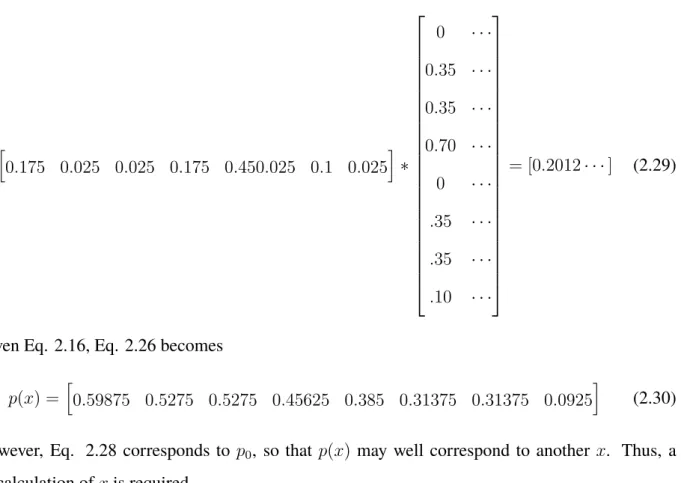
2.4.3 Frequency-dependent Transition Probability

The addition of frequency-dependence on the transition probability matrix requires a bit more re-finement to the steps previously presented. Now there is an additional complexity that,

p(x) = p0−

h

x·Ai (2.26)

where the 8x8 matrixAshould contain non-negative values and h

x·A i

< p0.

The example ofAused is:

A=                        

0 0 0 0 0 0 0 0

.35 .30 .30 .25 .20 .15 .15 .05

.70 .60 .60 .50 .40 .30 .30 .10

0 0 0 0 0 0 0 0

.35 .30 .30 .25 .20 .15 .15 .05

.70 .60 .60 .50 .40 .30 .30 .10

                        (2.27)

Note that the 1st _and₅th _{rows in Eq. (2.27) correspond to eco-friendly playing strategies:} _xt

1 and

xt

5. As an example of how Eq. 2.26 works, if

x=h0.175 0.025 0.025 0.175 0.450.025 0.1 0.025

i

(24)

then, for the first entry of the 1x8 arrayx∗.A:

h

0.175 0.025 0.025 0.175 0.450.025 0.1 0.025

i ∗                        

0 · · ·

0.35 · · ·

0.70 · · ·

0 · · ·

.35 · · ·

.10 · · ·

                       

= [0.2012· · ·] (2.29)

Given Eq. 2.16, Eq. 2.26 becomes

p(x) =h0.59875 0.5275 0.5275 0.45625 0.385 0.31375 0.31375 0.0925

i

(2.30)

However, Eq. 2.28 corresponds to p0, so that p(x) may well correspond to another x. Thus, a

re-calculation ofxis required.

The entire process flows as follows: I first choose a random set of numbers for theXt₁and Xt

2matrices keeping Eq. (2.17) in mind. I then use these matrices to obtain both the intermediatey

vector as well asp(x). yandp(x)are used to solve forQ(or vector ofQin the general case). This

leads tox∗.

Figure 2.3: A flowchart showing the beginning of the iterative process involved in

(25)

Figure 2.4: A flowchart showing the equations used to begin the iterative process. x

comes from the random sampling described in Section 2.4.1.

This process is repeated again and again (as seen in Fig. 2.3, with corresponding equations in Fig. 2.4) resulting in a vector of values: Q = [Q1, Q2, . . . , Qn−1, Qn] wheren is the iteration

number of the ‘Q’-loop. These values exhibit linear convergence and so the loop continues until

there is a trivial difference betweenQn+1 andQn, calculated via basic subtraction.

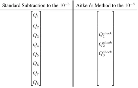
To make the algorithm faster, I increase the speed of the convergence of this sequence through the use of the ‘Aitken’s ∆2 method’ (Equation 2.14 in Burden and Faires (2010)) which

here takes the form,

Qcheck =Qn−

(Qn+1−Qn)2

Qn+2−2Qn+1+Qn

(2.31)

The condition I use to stop the iterations is

(Qcheck_m₊₁ −Qcheck_m )<1.0×10−8 (2.32)

Note that from Eq. (2.31),m6=nsincenmust reachn = 3beforeQcheck_m₌₁ can be found.

Thus, instead of subtracting every subsequentQ, I instead use Eq. (2.31) which

(26)

Standard Subtraction to the10−6 Aitken’s Method to the10−8

                    Q1 Q2 Q3 Q4 Q5 Q6 Q7 Q8                                         Qcheck 1 Qcheck 2 Qcheck 3                    

Table 2.1: Method for Determining the ‘true’ Q. In this example (based on initial calculation done

(27)

3. Results & Discussion

3.1 Type I Games

In addition to providing the foundation for the development of the algorithm, Type I games provide an interesting insight into the effects of the frequency matrix on dynamic competitive games.

Figure 3.1: A line plot for a Type I Game with non-FD stage payoffs.

The line plot (as seen in Fig. 3.1 for example) was created to give as clear an idea as possible as to the shape of the reward set inR2. It was made by setting 2 out of the 4 elements ofxvalues in

(28)

Page 20 Chapter 3. Results & Discussion

Figure 3.2: A scatter plot for a Type I Game with non-FD stage payoffs.

β−distribution, I obtain the line connecting(28,14)to(24,24). That is,

θt[pl1, pl2] = 0×(16,16) + 0×(14,28) +xt3×(28,14) +x

t

4×(24,24) (3.1)

for allt = {1· · · , T}In cases of the line plotTL = 20,000. For the scatter plots,TS = 50,000.

TL 6=TS for the simple reason that, with so many zero values created when generating a line plot,

the extra30,000add nothing new to these images.

The scatter plot version of Fig. 3.1 is seen in Fig. 3.2. Through it, one is able to visualise that for random samples of X∞ whentis large, there are higher concentrations of rewards closer

to the midpoint of the lines provided in the line plot.

Type I FD Game

The plot in Fig. 3.3 is particularly insightful. By manipulatingF D1, we can see how the reward set

shifts as the rewards it represents becomes increasingly influenced byF DI. I did this by inserting

a dummy variableα ∈[0,1]into Eq. (2.12) such that:

F DI = 1−

α

4(x2+ 2x3)− 2α

3 x4 (3.2)

By increasing theαthrough 5 runs of the algorithm (i.e. 5 different games), I create 5 different sets

of rewards, each with its own visual characteristics. As the onlyxi that remains unaffected isx1,

(29)

3.1 Type I Games Page 21

Figure 3.3: Line plots of 5 Type I games indicating the change in reward sets from

one game to the next. As the effect of the F DI function on the reward sets increase

from game to game, the reward space folds over so that the maximum upper right point

becomes the lowest, lower left point. This is done by increasing the value ofαin Eq.

(3.2). The extremesα= 0andα= 1are shown in Fig. 3.4.

Figure 3.4: The scatter plots compare the reward set of a Type I non-FD game

(north-east in red) and the reward set of a Type I FD game (south-west in blue)

(30)

set itselffolds overon the long term (Pareto inferior) point(16,16)so that it becomes the maximum

point in the final run of the algorithm whereα = 1. In Fig. 3.3 we see this as(24,24)reduces,

becoming(4,4).

Thus within this setup, one can say that with constant abuse of a common-pool resource over time, the Pareto superior point reduces in value till it becomes the Pareto inferior point. This new Pareto inferior point is still larger than the new Pareto superior point which has become even smaller.

Note that Fig. 3.4 is in keeping with a linear-reducing shift of the rewards as seen in Fig. 1 of Joostenet al.(2003).

3.2 Type II Games

Recall that Type II games are those in which there are two states that possess frequency-dependent payoffs and frequency-independent transition probabilities: Type II parameters are[θ(x), p0].

Figure 3.5: The (red) line plot to the north-east is that of the Type II non-FD game. The

blue line plot to the south-west is the Type II FD game. The dots indicate the location

of the stage payoffs ofS1andS2.

Manipulating the number of zero elements as described earlier allows for the visualization of different aspects of the reward set. In Fig. 3.5, two elements in X∞_i and 1 element in X∞_j

(31)

3.2 Type II Games Page 23

X∞₁ andX∞₂ are set to zero.

Figure 3.6: Here is a filled 2D version of the reward set when the stage payoffs are

non-FD. Twoxvalues in each state’s frequency matrix are set to zero here. The dots

indicate the location of the stage payoffs ofS1andS2.

Figure 3.7: Here is an entire reward set when the stage payoffs are FD. Twoxvalues

in each state’s frequency matrix are set to zero here. The dots indicate the location of

the stage payoffs ofS1andS2.

(32)

(a) 1000 iterations (b) 2500 iterations

Figure 3.8: Type II Game. Cropped images of scatter plots of reward sets for (left)

1000 iterations and (right) 2500 iterations atop the line plots of the Type II non-FD

reward space. The area of highest concentration is close to the north-east face of the

reward set.

and retains some of its lower-valued non-FD reward pairs.

By changing the number of iterations in a game, as in Figures 3.8 and 3.9, the areas of highest concentration (highest probability ’best for both’ points) can be determined. For the non-FD version, it lies around (14, 14). For the FD version it lies lower, around (10, 10).

It should also be noted that this area of highest concentration forms around a central region where the majority of the outlines intersect. As this inner region stretches during the transition from non-FD to FD, so too does the highest concentration of ‘best for both’ points.

In bothF Dand non-F Dcases, both players seem to have equally likely chances of

gain-ing a better payoff than their opponent.

To summarise, the effect ofF DII,III in Type II games is such that:

1. it reduces the probability of higher (closer toS1) rewards,

2. it also reduces the amount by which a player can best their opponent,

3. it increases the volatility of the rewards2.

3.3 Type III Games

Type III games are those in which there are two states that possess both frequency-dependent pay-offs and transition probabilities: Type II parameters are [θ(x), p(x)]. The setup for obtaining the

2_{Volatility is defined as ‘the measure of the uncertainty about the rewards provided by the resource’ (Section 14.4}

(33)

3.3 Type III Games Page 25

Figure 3.9: Type II Game. Cropped images of scatter plot of reward sets for (left) 1000

iterations and (right) 2500 iterations atop the line plots of the Type II FD reward space.

The area of highest concentration is around the centre of the reward set.

variations in plots for Type III games is the same as that described for Type II games.

Figure 3.10: The broader line plot to the upper right (red) is the reward set for the

non-FD game. The lower left (and narrower) line plot (blue) is the reward set for the

FD game.

In this example, for Type 3 games, the frequency-dependency transition probability func-tionp(x)has resulted in a situation vaguely similar to the Type I model where the non-F Dand FD

reward sets noticeably share a ‘best for both’ point. Unlike with the Type I, however, and similar to the Type II, the set does not fold over from this point but elongates the non-F Dfrom it to form

theF D reward set. A visual determination puts this point around (14, 14). Thus the lowest ‘best

(34)

‘best for both’ point going well below the lowest ‘best for both’ point ofS2.

Figure 3.11: Here is an entire reward set when the stage payoffs are non-FD. Two

x values in each state’s frequency matrix are set to zero here. The dots indicate the

location of the stage payoffs ofS1andS2.

On examining the regions of highest concentration, one can see from Fig 3.13 and Fig. 3.14 that the FD version has increased chances of lower rewards; much more so that its Type II counterpart. This seems to correspond with the elongation of the region of highest concentration south-westward. This means that the central region of the reward set in a Type III game is signific-antly affected by a frequency-dependence on the transition probability.

Figure 3.13: Type III Game. Cropped images of scatter plots of reward sets for (left)

1000 iterations and (right) 2500 iterations atop the line plots of the Type III non-FD

reward set. The area of highest concentration is around the centre the reward set,

(35)

3.3 Type III Games Page 27

Figure 3.12: Here is an entire reward set when the stage payoffs are FD. Twoxvalues

in each state’s frequency matrix are set to zero here. The dots indicate the location of

the stage payoffs ofS1andS2.

Figure 3.14: Type III Game. Cropped images of scatter plots of reward sets for (left)

1000 iterations and (right) 2500 iterations atop the line plots of the Type 3 FD reward

set. The area of highest concentration is in the bottom third of the set and extends both

to the south-west and to the north east.

To summarise, in the example of Type III games modeled here,

1. F D andp(x)reduces the amount by which a player can best their opponent,

2. p(x)further increases the volatility of the rewards compared to(F D, p0)as seen in the Type

II games,but

3. possesses the same ‘best for both’ maximum for both the FD and non-FD stage reward

(36)

4. Most importantly,the combination ofF DII,IIIandp(x)significantly reduces the probability

(37)

4. Conclusion

I have created a set of algorithms that allows for the representation of large sets of jointly-convergent pure strategy rewards for a large variety of stochastic games (with a repeated game being considered a special type of stochastic game). The .m files are provided in the Appendix of this document. Using Eq. (2.9) I calculate reward pairs for multiple stages. It is possible to plot these reward pairs inR2to visualise a game’s reward set.

With the use of anF Dfunction, it is possible to differentiate between stage rewards that

are affected by the frequency with which past actions have occurred, and those that are not so affected. It is also possible to differentiate between games in which the probability of moving from one state to another is dependent on the frequency of past actions and those that are not, through the use of a frequency-dependent transition probability function.

The model developed here is geared toward 2-player, 2-action, 2-state stochastic games. Aside from these specifications, it is actually quite broad, able to handle any type ofF Dfunction

and possibly non-linearp(x)functions as well. The use of theF Dis entirely optional and the user

can not only manipulate whether or not the stage rewards (or transition probabilities) are frequency-dependent, but can also consider the intermediate levels where these rewards (probabilities) vary in thedegreeto which they are affected.

The example used to ensure the code’s functionality was the fishery war which is a ‘

Com-mons’-type social dilemma. Here, the two players are encouraged toward actions that will harm

(38)

Page 30 Chapter 4. Conclusion

of highest rewards lie in the centre of the reward set’s diagrammatic form. When theF D function

is reduced linearly, the reward set folds over so that the Pareto inferior ‘best of both’ point of the initial reward space becomes the new Pareto superior ‘best of both’ point in the final reward set.

Results for Type II and Type III games were similar in most respects. F D stage payoffs

shifted the reward set to lower values, and reduced the difference in rewards in stages where a player obtained a reward higher than the opposing player. As frequency dependency increases the ‘length’ of the reward set, there is a corresponding increase in the volatility of the rewards that can be obtained.

The one major area of difference between the Type II and Type III games was the re-positioning of the region of highest concentration that sat lower in the reward set’s diagrammatic interpretation of the Type III model than that of the Type II, regardless ofF DII,III. Thus we can

conclude that an F D transition probability is a significant factor in the probability of obtaining

higher rewards.

Also, the Type III (FD) game shared a short term (Pareto superior) point with that of the Type III (non-FD) game.

4.1 Further Developments

Together with my supervisor, Reinoud Joosten, we are in the process of publishing the findings made in the Type III FD games, with new ideas still developing.

One major consideration throughout this project has been the classification of the differ-ent types of games. Recdiffer-ent discussions have led to the idea that, if repeated games are a type of stochastic game, then Table 1.1 contains an error in the ‘Play’ row where ‘repeated’ was considered as a separate class from ‘stochastic’. This led to the idea of Action-Independent Transition prob-ability matrices (A.I.T.), where the transition probprob-ability matrices in Eq. (2.15) are instead of a general form,

pS1

0 =





ω,(1−ω) ω,(1−ω)



 pS₀2 = 



ρ,(1−ρ) ρ,(1−ρ)



 (4.1)

where 0 ≤ ω, ρ ≤ 1. This way, no matter the action pair, the transition probabilities per state

remain unchanged.

(39)

4.2 Future Work Page 31

(2.25b):

Q(1−ω) =ρ(1−Q) (4.2a)

Q= ρ

1−ω+ρ (4.2b)

This need only be done once for the entire game asQhere is constant.

So we see that with the concept of AIT, unlike what was stated in the Methodology: a Type I gamecanexist with multiple reachable states.

4.2 Future Work

It is important to recognise that the results in the example may not necessarily hold for all types of social dilemma. What Icansay is that because one can model any type of social dilemma using

this code, the following additions may be of academic interest:

1. Compiling all .m files into a single code with input options for the user. 2. A three-player model will allow interesting visualizations of the rewards. 3. Any of the following:

(a) changing the type of social dilemma, Komorita and Parks (1996) give an in depth look into a few of the more well-known social dilemmas),

(b) changing the quality of the F D functions (F D1 and F D2,3) or transition probability

p(x) function, to a non-linear (though still continuous) function, or to more involved

continuous linear functions like Henry Hamburger’s ‘Give Some’ games (see p. 12 in Komorita and Parks (1996)),

(c) alter the frequency matrices to reflect specific strategies.

4. Creating a three-state system ofS1,S2andS3. (with linear algebra, this should make moving

to multi-state modeling much easier).

5. Parallel computing iterationst= 1, ..., T can increase speed.

6. Consider the effects of temporarily absorbing states.

4.3 Final Thoughts

(40)

Page 32 Chapter 4. Conclusion

visualization of rewards, allowed through the algorithm I have created, presents a clear picture of the effects of abusing common-pool systems. I leave it as a project for the interested reader to add his or her functions to give realistic considerations of scenarios in which long term goals lead from low states to high ones: a much more positive spin than the scenario presented in this thesis.

Secondly, in the introduction I mentioned the efficiency of the Joosten and Meijboom (2010) Type III [θ0, p(x)] game. My focus on communicating states (states that will never have

transition probabilities equal to 0), has allowed me to develop a much more efficient algorithm to model social dilemmas than that of Joosten and Meijboom. As shown in theFuture Worksection,

it is possible to adapt the code to consider absorbing states. However, whether or not the increase in processing time (as the algorithm searches for appropriatexvalues to fit a uniqueflow equation)

will be proportional to the increase experienced by Joosten and Meijboom remains to be seen, but seems unlikely.

(41)

References

Brenner, Thomas and Ulrich Witt. ‘Melioration learning in games with constant and frequency-dependent payoffs’. In:Journal of Economic Behavior & Organization50 (2003), pp. 429–

448. url:http://dx.doi.org/10.1016/S0167-2681(02)00034-3.

Burden, Richard L. and J. Douglas Faires.Numerical analysis. 9th ed. Brooks/Cole, 2010.

Hardin, Garrett. ‘The tragedy of the commons’. In:Science Magazine162.3859 (Dec. 1968), pp. 1243–

1248. url:http://science.sciencemag.org/content/162/3859/1243.full.

Hull, John C.Options, futures, and other derivatives. 8th ed. Brooks/Cole, 2012.

Joosten, Reinoud. ‘Small fish wars: a new class of dynamic fishery-management games’. In: The

IUP Journal of Managerial EconomicsV.4 (Nov. 2007), pp. 17–30.

— ‘Strong and weak rarity value: resource games with complex price–scarcity relationships’. In:Dynamic Games and Applications6.1 (Mar. 2016), pp. 97–111. url:http://link.

springer.com/article/10.1007/s13235-015-0136-4.

Joosten, Reinoud, Thomas Brenner and Ulrich Witt. ‘Games with frequency-dependent stage pay-offs’. In: International Journal of Game Theory 31.4 (Jan. 2003), pp. 609–620. url:

https://doi.org/10.1007/s001820300143.

Joosten, Reinoud and Robin Meijboom. ‘Stochastic games with endogenous transitions’. In:Papers

on Economics & Evolution4.1024 (Nov. 2010), pp. 1–29. url:https://papers.econ.

(42)

Page 34 REFERENCES

Komorita, Samuel S. and Craig D. Parks. Social dilemmas. Social Psychology Series. Westview

Press, 1996.

Levhari, David and Leonard J. Mirman. ‘The great fish war: an example using a dynamic cournot-nash solution’. In:The Bell Journal of Economics11.1 (Spring 1980), pp. 322–334. url:

http://www.jstor.org/stable/3003416.

Mahohoma, W. ‘Stochastic games with frequency-dependent stage payoffs’. diploma thesis. Maastricht University, Aug. 2014. url:https://dke.maastrichtuniversity.nl/gm.schoenmakers/

wp-content/uploads/2015/10/Master-Thesis-Mahohoma-SQ.pdf.

Peters, Hans.Game theory. A multi-leveled approach. Springer, 2008.

Ross, Sheldon M.Introduction to probability models. 10th ed. Elsevier, 2010.

Van Lange, Paul A. M., Jeff Joireman, Craig D. Parks and Eric Van Dijk. ‘The psychology of social dilemmas: a review’. In: Organizational Behavior and Human Decision Processes 120

(Nov. 2013), pp. 125–141. url:http://dx.doi.org/10.1016/j.obhdp.2012.11.

(43)

(44)

(45)

A Algorithm 1: Type 1 Game Page 37

A

Algorithm 1: Type 1 Game

1 %Type 1 Game 2 %(0 <= alpha <=1) . 3 c l e a r

4 %−−−[1] The p a y o f f v e c t o r s

5 A1 = [16 14 28 2 4 ] ' ;

6 B1 = [16 28 14 2 4 ] ' ;

7 %−−−[2] s t a g e l e v e l and s t o r a g e

8 T=100000;

9 Payoff1 = z e r o s (T , 1 ) ;

10 Payof f2 = z e r o s (T , 1 ) ;

11 x = z e r o s ( 4 , 1 ) ;

12 r = z e r o s ( 4 , 1 ) ;

13 prompt = ' What i s a l p h a ? ';

14 a l p h a = i n p u t ( prompt ) ;

15 f o r v =1:T

16 %−−−[3] Frequency v e c t o r x ( s c a t t e r )

17 f o r i = 1 : 4

18 r ( i ) = b e t a r n d ( 0 . 5 , 0 . 5 ) ;

19 end

20 Norm_val = sum ( r ) ;

21 f o r i = 1 : 4

22 x ( i ) = r ( i ) / Norm_val ;

23 end

24 %%%∗∗∗∗

25 %−−−[3] Frequency v e c t o r x ( o u t l i n e )

26 %f o r i = 1 : 2 ;

27 % r ( i ) = b e t a r n d ( 0 . 5 , 0 . 5 ) ; 28 %end

29 %Norm_val = sum ( r ) ; 30 %f o r i = 1 : 2

31 % x_a ( i ) = r ( i ) / Norm_val ; 32 %end

33 %x_b = [ x_a ( 1 ) x_a ( 2 ) 0 0 ] ' ;

34 %x = x_b ( randperm ( l e n g t h ( x_b ) ) ) ; %r a n d o m i s e s x_b 35 %%∗∗∗∗

(46)

Page 38

37 FD = 1−a l p h a ∗ 0 . 2 5 ∗ ( x ( 2 ) + 2∗x ( 3 ) )−a l p h a ∗ ( 2 / 3 ) ∗x ( 4 ) ;

38 %−−−[5] Sta g e p a y o f f v e c t o r s

39 V_p1 = x . ∗ A1 ;

40 V_p2 = x . ∗ B1 ;

41 Payoff1 ( v ) =FD∗sum ( V_p1 ) ;

42 Pa yoff2 ( v ) =FD∗sum ( V_p2 ) ;

43 end

44 %−−−[6] p l o t

45 f i g u r e ( 1 )

46 p l o t ( Payoff1 , Payoff2 , ' ∗ r ' , ' MarkerSize ' , 1)

47 x l a b e l ( ' P l a y e r 1 ')

48 a x i s ( [ 5 30 5 3 0 ] )

49 y l a b e l ( ' P l a y e r 2 ')

50 t i t l e ( [ ' Reward Space . T= ' num2str (T) ' i t e r a t i o n s . '] )

B

Algorithm 2: Type 2 Game

1 %2−s t a t e s t o c h a s t i c game with p0 . c o n s t p a y o f f ( a l p h a =0) , FD−p a y o f f ( a l p h a =1) .

2 c l e a r

3 %−−−[1] The p a y o f f v e c t o r s and p0

4 A1 = [16 14 28 24 4 3 . 5 7 6 ] ' ; %v e c t o r 5 B1 = [16 28 14 24 4 7 3 . 5 6 ] ' ; %v e c t o r

6 p = [ 0 . 8 0 . 7 0 . 7 0 . 6 0 . 5 0 . 4 0 . 4 0 . 1 5 ] ' ; %v e c t o r 7 %p i s t h e p r o b a b i l i t y of moving t o S1

8

9 %−−−[2] s t a g e l e v e l and s t o r a g e

10 T = 50000; %1000000; 11 x = z e r o s ( 8 , 1 ) ;

12 x_a = z e r o s ( 8 , 1 ) ;

13 x s t a r = z e r o s ( 8 , 1 ) ;

14 r = z e r o s ( 8 , 1 ) ;

15 y = z e r o s ( 8 , 1 ) ;

16 yp = z e r o s ( 4 , 1 ) ;

17 yp_not = z e r o s ( 4 , 1 ) ;

(47)

B Algorithm 2: Type 2 Game Page 39

19 v_p2 = z e r o s ( 8 , 1 ) ;

20 payoff_p1 = z e r o s (T , 1 ) ;

21 payoff_p2 = z e r o s (T , 1 ) ;

22

25

26 f o r t = 1 : T

27 %−−−[3] Frequency v e c t o r x ( s c a t t e r )

28 f o r i = 1 : 8

29 r ( i ) = b e t a r n d ( 0 . 5 , 0 . 5 ) ;

30 end

31

32 f o r i = 1 : 8

33 x ( i ) = r ( i ) / sum ( r ) ;

34 end

35 %%∗∗∗∗

36 %%−−−[3] Frequency v e c t o r x ( o u t l i n e )

37 %f o r i = 1 : 3 %

38 % r ( i ) = b e t a r n d ( 0 . 5 , 0 . 5 ) ; 39 %end

40 %

41 %Norm_val = sum ( r ) ; 42 %

43 %f o r i = 1 : 3 %

44 % x_a ( i ) = r ( i ) / Norm_val ; 45 %end

46 %

47 %x_b1 = [ x_a ( 1 ) x_a ( 3 ) 0 0] ';% 48 %x_b2 = [ x_a ( 2 ) 0 0 0] ';% 49 %

50 %x_c1 = x_b1 ( randperm ( l e n g t h ( x_b1 ) ) ) ; %%r a n d o m i s e s p o s i t i o n s of x_b 51 %x_c2 = x_b2 ( randperm ( l e n g t h ( x_b2 ) ) ) ;

52 %

53 %f o r i =1:8 54 % i f i < 5

(48)

Page 40

56 % e l s e

57 % x ( i ) = x_c2 ( i−4) ;

58 % end 59 %end

60 %%∗∗∗∗ 61

62 %−−−[4] I n t e r m e d i a t e y v e c t o r and Q

63 f o r i =1:4

64 y ( i ) = x ( i ) / ( sum ( x ( 1 : 4 ) ) ) ;

65 end

66 f o r i =5:8

67 y ( i ) = x ( i ) / ( sum ( x ( 5 : 8 ) ) ) ;

68 end

69 f o r i = 1 : 4

70 yp_not ( i ) = y ( i ) ∗(1−p ( i ) ) ;

71 yp ( i ) = y ( i +4) ∗p ( i +4) ;

72 end

73 Q = sum ( yp ) / ( sum ( yp ) + sum ( yp_not ) ) ;

74 Q_not = 1−Q;

75

76 %−−−[5] S o l v i n g f o r x∗

77 f o r i = 1 : 4

78 x s t a r ( i ) = Q∗y ( i ) ;

79 end

80 f o r i = 5 : 8

81 x s t a r ( i ) = Q_not∗y ( i ) ;

82 end

83

84 %−−−[6] FD e q u a t i o n

85 FD = 1− a l p h a ∗ 0 . 2 5 ∗ ( x s t a r ( 2 ) + x s t a r ( 3 ) )...

86 −0.5∗ a l p h a ∗( x s t a r ( 6 ) + x s t a r ( 7 ) ) − ( 1 / 3 ) ∗ a l p h a ∗ x s t a r ( 4 ) −(2/3) ∗ a l p h a ∗

x s t a r ( 8 ) ;

87 f o r i = 1 : 8

88 v_p1 ( i ) = x s t a r ( i ) ∗A1( i ) ;

89 v_p2 ( i ) = x s t a r ( i ) ∗B1 ( i ) ;

90 end

(49)

C Algorithm 3: Type 3 Game Page 41

92 %−−−[7] Stag e p a y o f f v e c t o r

93 payoff_p1 ( t ) = FD∗sum ( v_p1 ) ;

95 end

96

97 %−−−[8] p l o t

98 f i g u r e ( 1 )

99 s c a t t e r (A1 , B1 , ' f i l l e d ')

100 hold on

101 p l o t ( payoff_p1 , payoff_p2 , ' o ', ' MarkerSize ' , 1 ,...

102 ' MarkerFaceColor ' , ' r ', ' MarkerEdgeColor ', ' r ')

103 x l a b e l ( ' P l a y e r 1 ')

104 y l a b e l ( ' P l a y e r 2 ')

105 t i t l e ( [ ' Type 2 Game Reward Space . T = ' num2str (T) ' i t e r a t i o n s '] )

106 hold o f f

C

Algorithm 3: Type 3 Game

1 c l e a r

2 %

3 A1 = [16 14 28 24 4 3 . 5 7 6 ] ' ;

4 B1 = [16 28 14 24 4 7 3 . 5 6 ] ' ;

5 p = [ 0 . 8 0 . 7 0 . 7 0 . 6 0 . 5 0 . 4 0 . 4 0 . 1 5 ] ;

6 x = z e r o s ( 1 , 8 ) ;

7 r = z e r o s ( 8 , 1 ) ;

8 y = z e r o s ( 8 , 1 ) ;

9 x s t a r = z e r o s ( 1 , 8 ) ;

10 x_a = z e r o s ( 8 , 1 ) ;

11 yp = z e r o s ( 4 , 1 ) ;

12 yp_not = z e r o s ( 4 , 1 ) ;

13 v_p1 = z e r o s ( 1 , 8 ) ;

14 v_p2 = z e r o s ( 1 , 8 ) ;

15 T = 500000;

16 payoff_p1 = z e r o s (T , 1 ) ;

(50)

Page 42

18

19 matrixA = [ 0 . 0 0 0 . 0 0 . 0 0 .0 0 0 . 0 0 . 00 0. 00 0 . 0 0 ;

20 0 . 3 5 0 . 3 0 . 3 0 .2 5 0 . 2 0. 15 0. 15 0 . 0 5 ;

21 0 . 3 5 0 . 3 0 . 3 0 .2 5 0 . 2 0. 15 0. 15 0 . 0 5 ;

22 0 . 7 0 0 . 6 0 . 6 0 .5 0 0 . 4 0. 30 0. 30 0 . 1 0 ;

23 0 . 0 0 0 . 0 0 . 0 0 .0 0 0 . 0 0. 00 0. 00 0 . 0 0 ;

24 0 . 3 5 0 . 3 0 . 3 0 .2 5 0 . 2 0. 15 0. 15 0 . 0 5 ;

25 0 . 3 5 0 . 3 0 . 3 0 .2 5 0 . 2 0. 15 0. 15 0 . 0 5 ;

26 0 . 7 0 0 . 6 0 . 6 0 .5 0 0 . 4 0. 30 0. 30 0 . 1 0 ] ;

27

30

31 f o r t = 1 : T

32

33 Q_checker

34

35 FD = 1− a l p h a ∗ 0 . 2 5 ∗ ( x s t a r ( 2 ) + x s t a r ( 3 ) ) −0.5∗ a l p h a ∗( x s t a r ( 6 ) + x s t a r ( 7 ) )...

36 − ( 1 / 3 ) ∗ a l p h a ∗ x s t a r ( 4 ) −(2/3) ∗ a l p h a ∗ x s t a r ( 8 ) ;

37 f o r i = 1 : 8

38 v_p1 ( i ) = x s t a r ( i ) ∗A1( i ) ;

39 v_p2 ( i ) = x s t a r ( i ) ∗B1 ( i ) ;

40 end

43 end

44

45 f i g u r e ( 1 )

46 s c a t t e r (A1 , B1 , ' f i l l e d ')

47 hold on

48 p l o t ( payoff_p1 , payoff_p2 , ' o ' ,' MarkerSize ' , 1 ,...

49 ' MarkerFaceColor ' , [ 0 . 5 0 . 5 0 . 5 ] , ' MarkerEdgeColor ' , [ 0 . 5 0 . 5 0 . 5 ] )

50 x l a b e l ( ' P l a y e r 1 ')

51 y l a b e l ( ' P l a y e r 2 ')

52 t i t l e ( [ ' Type 3 FD Game Reward Space . T = ' num2str (T) ' i t e r a t i o n s '] )

(51)

D Algorithm 4: Q Checker Page 43

D

Algorithm 4: Q Checker

1 %loop t o match px and x ∗ . i n s e r t i n t y p e 3 a l g o r i t h m 2 %−−−[1] Frequency v e c t o r x ( s c a t t e r )

3 % f o r i = 1 : 8

4 % r ( i ) = b e t a r n d ( 0 . 5 , 0 . 5 ) ; 5 % end

6 % f o r i = 1 : 8

7 % x ( i ) = r ( i ) / ( sum ( r ) ) ; 8 % end

9 % %−−−

10 %−−−[1] Frequency v e c t o r x ( o u t l i n e )

11 f o r i = 1 : 3

12 r ( i ) = b e t a r n d ( 0 . 5 , 0 . 5 ) ;

13 end

14 Norm_val = sum ( r ) ;

15 f o r i = 1: 3 %

16 x_a ( i ) = r ( i ) / Norm_val ;

17 end

18 x_b1 = [ x_a ( 1 ) x_a ( 3 ) 0 0 ] ' ;% 19 x_b2 = [ x_a ( 2 ) 0 0 0 ] ' ;%

20 x_c1 = x_b1 ( randperm ( l e n g t h ( x_b1 ) ) ) ; %r a n d o m i s e s p o s i t i o n s of x_b 21 x_c2 = x_b2 ( randperm ( l e n g t h ( x_b2 ) ) ) ;

22 f o r i =1:8

23 i f i < 5

24 x ( i ) = x_c1 ( i ) ;

25 e l s e

26 x ( i ) = x_c2 ( i−4) ;

27 end

28 end

29 % %−−−

30 %−−−[2] I n t e r m e d i a t e y v e c t o r , Q and x∗

31 f o r i = 1 : 4

32 y ( i ) = x ( i ) / ( sum ( x ( 1 : 4 ) ) ) ;

33 end

34 f o r i =5:8

35 y ( i ) = x ( i ) / ( sum ( x ( 5 : 8 ) ) ) ;

(52)

Page 44

37 px = p − x∗ matrixA ;

38 f o r w = 1 : 4

39 f o r i = 1 : 4

40 yp ( i ) = y ( i +4) ∗px ( i +4) ;

41 yp_not ( i ) = y ( i ) ∗(1−px ( i ) ) ;

42 end

43 Q =( sum ( yp ) ) / ( ( sum ( yp_not ) ) + ( sum ( yp ) ) ) ;

44 Q_not = 1−Q;

45 Q_vec (w) = Q;

46 f o r i =1:4

47 x s t a r ( i ) = Q∗y ( i ) ;

48 end

49 f o r i = 5: 8

50 x s t a r ( i ) = Q_not∗y ( i ) ;

51 end

52 px = p − x s t a r ∗ matrixA ;

53 end

54 Q_check_1 = Q_vec ( 1 )− ( ( Q_vec ( 2 )−Q_vec ( 1 ) ) ^2) / ( Q_vec ( 3 )− 2∗Q_vec ( 2 ) + Q_vec ( 1 )

) ;

55 Q_check_2 = Q_vec ( 2 )− ( ( Q_vec ( 3 )−Q_vec ( 2 ) ) ^2) / ( Q_vec ( 4 ) − 2∗Q_vec ( 3 ) + Q_vec

( 2 ) ) ;

56 d i f f = Q_check_1 − Q_check_2 ;

57

58 wh ile d i f f > abs (1 e−8)

59

60 Q_check_1 = Q_check_2 ;

61 f o r i = 1 : 4

62 yp ( i ) = y ( i +4) ∗px ( i +4) ;

63 yp_not ( i ) = y ( i ) ∗(1−px ( i ) ) ;

64 end

65 Q =( sum ( yp ) ) / ( ( sum ( yp_not ) ) + ( sum ( yp ) ) ) ;

66 Q_not = 1−Q;

67 Q_vec (w+1) = Q;

68 f o r i =1:4

69 x s t a r ( i ) = Q∗y ( i ) ;

70 end

(53)

D Algorithm 4: Q Checker Page 45

72 x s t a r ( i ) = Q_not∗y ( i ) ;

73 end

74 px = p − x s t a r ∗ matrixA ;

75 Q_check_2 = Q_vec (w−1)...

76 − ( ( Q_vec (w)−Q_vec (w−1) ) ^2) / ( Q_vec (w+1) − 2∗Q_vec (w) + Q_vec (w−1) ) ;

77 d i f f = Q_check_1 − Q_check_2 ;

78 w = w+1;

Computations in Stochastic Game Theory : large sets of rewards in games with communicating states and frequency dependent transition probabilities and stage payoffs

Faculty of Behavioural

Management & Social Sciences

M.Sc. Program: Industrial Engineering & Management

Master Thesis

Computations in Stochastic Game Theory

Large sets of rewards in games with communicating states

and frequency-dependent transition

probabilities and stage payoffs

Acknowledgements

Abstract

Contents

1

Introduction

2

Methodology

3

Results & Discussion

4

Conclusion

Appendices

List of Figures

2.1

2.2

2.3

2.4

3.1

3.2

3.3

3.4

3.5

3.6

3.7

3.8

3.9

3.10

3.11

3.13

3.12

1. Introduction

1.1

Game Theory in Social Dilemmas

1.2

Thesis Aim and Paper Organisation

2. Methodology

2.1

Necessary Conditions

2.2

Repeated Games

2.3

Stochastic Games

2.4

Computing Type II and Type III Games

3. Results & Discussion

3.1

Type I Games

3.2

Type II Games

3.3

Type III Games

4. Conclusion

4.1

Further Developments

4.2

Future Work

4.3

Final Thoughts

References

A

Algorithm 1: Type 1 Game

B

Algorithm 2: Type 2 Game

C

Algorithm 3: Type 3 Game

D

Algorithm 4: Q Checker