Proposing a New Method to Improve Feature Selection with Meta Heuristic Algorithm and Chaos Theory

Proposing a New Method to Improve Feature Selection

with Meta-Heuristic Algorithm and Chaos Theory

Mohammad Masoud Javidi

Department of Computer Science, Shahid Bahonar

University of Kerman, Kerman, Iran

Nasibeh Emami

Department of Computer Science, Kosar University

of Bojnord, Bojnord, Iran

ABSTRACT

Finding a subset of features from a large data set is a problem that arises in many fields of study. It is important to have an effective subset of features that is selected for the system to provide acceptable performance. This will lead us in a direction that to use meta-heuristic algorithms to find the optimal subset of features. The performance of evolutionary algorithms is dependent on many parameters which have significant impact on its performance, and these algorithms usually use a random process to set parameters. The nature of chaos is apparently random and unpredictable; however it also deterministic, it can suitable alternative instead of random process in meta-heuristic algorithms.

Keywords

Feature selection, Classification, Meta-heuristic algorithm, Binary particle swarm optimization, Chaos theory.

1.

INTRODUCTION

Feature selection is essential in analyzing large dataset, especially being a preprocessing step to reducing dimensionality, removing irrelevant features, reducing storage requirements and enhancing output comprehensibility [1]. Applications of feature selection can be noted pattern recognition [2-5], machine learning [6] and data mining [7]. The term of feature selection is taken to refer to algorithms that the input from them is feature set and output of them is a subset of input feature set [8]. General procedure of feature selection algorithms is creating a subset, evaluate it, and loop until a stop criterion is satisfied. Then the subset extracted is validated by the classifier algorithm [9, 10].

Feature selection algorithms can be classified into two categories based on their evaluation procedure [11, 12]:

 Filter: the quality of a subset of features is determined by using characteristics of that subset, without use any learning algorithm.

 Wrapper: To determining the adequacy of a subset of features, use learning algorithm and performance of learning algorithm is a measure to select subset or not.

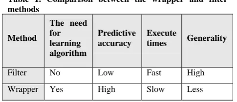
In [13] there is a good explanation of filter and wrapper methods. We describe them here and give a summary of property of filter and wrapper method in Table 1.

Since wrapper methods use a learning algorithm to evaluate each feature subset; are expensive to run but give better results (predictive accuracy) than filters. Also these methods are less general than filters and must be re-run when switching from one learning algorithm to another. Filters don’t use learning algorithm they are many times faster than wrappers. Filters do not require re-execution of different learning algorithms. Filters can provide a good starting feature subset for a wrapper method. A process that is likely to result in a

shorter, and hence faster, search for the wrapper. The Table 1 shows a summary comparison between the wrapper and filter methods.

Table 1. Comparison between the wrapper and filter methods

Method

The need for learning algorithm

Predictive accuracy

Execute

times Generality

Filter No Low Fast High

Wrapper Yes High Slow Less

Search is an important issue in feature selection problem because the whole search space for optimization contains all possible subsets of features, the size of such space is 2d. Where d is the number of original features. Because of this space typically feature selection algorithms include heuristic or random search strategies to avoid this prohibitive complexity [14]. Nevertheless development of a highly accurate and fast search algorithm for the selection of optimal feature subset is an open issue [15]. A wrapper feature selection for classification proposed in this paper. The proposed algorithm is based on one new binary particle swarm optimization and chaos inertia weight and use the K-nearest neighbor (K-NN) method with leave-one-out cross-validation as a classifier for evaluating classification accuracies.

This paper organized in 6 sections: Section 2 reviews some previous studies in the area of feature selection, section 3 is preliminaries about proposed method. Proposed method will explain in section 4, implementation and result coming in section 5 and finally conclusion coming in section 6.

2.

RELATED WORKS

Some feature selection techniques reviewed in this section. Several common feature selection methods are named here. In previous section has mentioned feature selection methods generally fall into two categories: filter and wrapper. Some filter approaches are: t-test [16], chi-square test [17], Wilcoxon Mann–Whitney test [18], mutual information [19], Pearson correlation coefficients [20] and principal component analysis [21] Relief [22], Focus [23], LVF [24], SCRAP [25], EBR [26], FDR [27] and etc.

 Greedy

 Randomized/Stochastic

Greedy wrapper approaches use less computer time than other wrapper methods. Sequential forward selection (SFS) [29, 30], is to start the search process with an empty set and successfully add features; and Sequential backward selection (SBS) [31, 32], is to start with a full set and successfully remove features; are the two most commonly used wrapper methods that use a greedy search strategy. The disadvantage of SFS and SBS is that they can easily be fall into local minima [15].

Stochastic algorithms developed for solving wrapper feature selection such as Ant Colony Optimization (ACO) [33,34], Genetic Algorithm (GA) [35, 36], Particle Swarm Optimization (PSO) [37, 38] .They are global search and cannot easily be trapped into local minima. They can produce the best solution by heuristic information but these algorithms are computationally expensive [15, 28].

In this paper we will introduce a wrapper feature selection method to search in exhausted feature space and find an optimal feature subset for classifier task. In the next section we introduce preliminaries of the proposed method.

3.

PRELIMINARIES

A new version of the binary particle swarm optimization with chaotic inertia weight are used in proposed algorithm. So the following is a more detailed description of particle swarm optimization, binary particle swarm optimization, new binary particle swarm optimization, and chaos theory for setting inertia weight and the classifier that used in proposed method.

3.1

Particle swarm optimization

Particle Swarm Optimization (PSO) was first suggested by Kennedy and Eberhart in 1995 [39]. PSO is a global optimization that is inspired by the social behavior of birds. It is a population based optimization technique, where a population is called a swarm [40]. A swarm consists of N particles moving around in a d-dimensional search space. The position of the ith particle can be represented by:

𝑥𝑖= 𝑥𝑖1, 𝑥𝑖2, … , 𝑥𝑖𝑑 𝑖 = 1,2, … , 𝑁

and for represented velocity of each particle we have: 𝑣𝑖= 𝑣𝑖1, 𝑣𝑖2, … , 𝑣𝑖𝑑 𝑖 = 1,2, … , 𝑁

The positions and velocities of the particles are confined within [𝑋𝑚𝑖𝑛, 𝑋𝑚𝑎𝑥]d and [𝑉𝑚𝑖𝑛, 𝑉𝑚𝑎𝑥]d respectively. Each

particle has a memory that keeps its previous best position: 𝑃_𝑏𝑒𝑠𝑡𝑖= 𝑃𝑏𝑒𝑠𝑡 𝑖1, 𝑃𝑏𝑒𝑠𝑡 𝑖2, … , 𝑃𝑏𝑒𝑠𝑡 𝑖𝑑 𝑖 = 1,2, … , 𝑁

In PSO, we have global best concept that it is the best position among all the particles in the population and can be represented by:

𝐺𝑏𝑒𝑠𝑡 = 𝐺𝑏𝑒𝑠𝑡 1, 𝐺𝑏𝑒𝑠𝑡 2, … , 𝐺𝑏𝑒𝑠𝑡 𝑑

At each iteration, the velocity and the position of each particle are updated according to its previous best position (P_best) and the global best position(G_best). Redefined formula are: 𝑣𝑖𝑑 𝑇 + 1 =𝑤 𝑣𝑖𝑑 𝑇

+ 𝐶1 𝑅𝑎𝑛𝑑1 𝑃𝑏𝑒𝑠𝑡 𝑖𝑑− 𝑥𝑖𝑑 𝑇

+𝐶2 𝑅𝑎𝑛𝑑2 𝐺_𝑏𝑒𝑠𝑡 − 𝑥𝑖𝑑(𝑇) (1)

𝑥𝑖𝑗 𝑇 + 1 = 𝑥𝑖𝑗 𝑇 + 𝑣𝑖𝑗 𝑇 + 1 (2)

Where j=1, 2, …, d. w is the inertia coefficient between [0, 1], C1, C2 are the acceleration constants, Rand1 and Rand2 are random number between [0, 1]. 𝑣𝑖𝑗 𝑇 + 1 and 𝑣𝑖𝑗(𝑇) are

velocities of the updated particle and the particle before being updated, respectively, 𝑥𝑖𝑗 𝑇 is the original particle position,

and 𝑥𝑖𝑗 𝑇 + 1 is the updated particle position [41].

PSO was presented to solve problems in continuous space; in discrete space problems Kennedy and Eberhart proposed binary version of PSO (BPSO) [42]. In BPSO the position of a particle is represented as the binary string and is randomly generated. In feature selection problem zero bit means unselected feature and bit with one value means that selected feature. The initial velocities are probabilities limited to a range of [0, 1] and velocity update by Eq (1) .If the velocity after updating in each dimension exceed𝑉𝑚𝑎𝑥, then the

velocity of that dimension is limited to 𝑉𝑚𝑎𝑥 (Eq. (3)). Both

𝑉𝑚𝑎𝑥and 𝑉𝑚𝑖𝑛 are user-specified parameters [41].

𝐼𝑓𝑣𝑖𝑗 𝑇 + 1 ∉ 𝑉𝑚𝑖𝑛 , 𝑉𝑚𝑎𝑥

𝑡ℎ𝑒𝑛 𝑣𝑖𝑗 𝑇 + 1 = max 𝑚𝑖𝑛 𝑉𝑚𝑎𝑥, 𝑣𝑖𝑗 𝑇 + 1 , 𝑉𝑚𝑖𝑛

𝑗 = 1,2, … , 𝑑 (3)

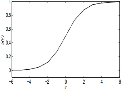
In order to update position of each particle, PSO should first transform the velocity vector into a probability vector through a sigmoid function [43]. Figure 1 shows sigmoid function.

Fig 1: Sigmoid function (Rostami and Nezamabadi 2006)

So Eq. (4) and Eq. (5) use for update position of each particle.

𝑆 𝑣𝑖𝑗 𝑇 + 1 = 1

1 + 𝑒−𝑣𝑖𝑗 𝑇+1 𝑗 = 1,2, … , 𝑑 (4)

𝑥𝑖𝑗 𝑇 + 1 = 1 𝑖𝑓 𝑟𝑎𝑛𝑑 < 𝑆 𝑣𝑖𝑗 𝑇 + 1

0 𝑂. 𝑊

𝑗 = 1,2, … , 𝑑 (5)

3.2

New binary particle swarm

optimization

In original BPSO the new position of each particle is based on the likelihood function (sigmoid function) that 𝑣𝑖𝑗(𝑇 + 1)

passes of the sigmoid function. Because of use this function in original BPSO, Rostami and Nezamabadi in [44] Objections were made on the original BPSO.

likelihood function.

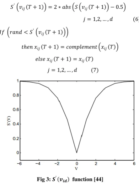
In Eq. (4) previous position of the particle to calculate the next position of the particle's position is not considered. To eliminate the disadvantage of BPSO, they proposed Eq. (6) and Eq. (7):

𝑆′ _𝑣

𝑖𝑗 𝑇 + 1 = 2 ∗ 𝑎𝑏𝑠 𝑆 𝑣𝑖𝑗 𝑇 + 1 − 0.5

𝑗 = 1,2, … , 𝑑 (6)

𝐼𝑓 𝑟𝑎𝑛𝑑 < 𝑆′ _𝑣

𝑖𝑗 𝑇 + 1

𝑡ℎ𝑒𝑛 𝑥𝑖𝑗 𝑇 + 1 = 𝑐𝑜𝑚𝑝𝑙𝑒𝑚𝑒𝑛𝑡 𝑥𝑖𝑗 𝑇

𝑒𝑙𝑠𝑒 𝑥𝑖𝑗 𝑇 + 1 = 𝑥𝑖𝑗 𝑇

𝑗 = 1,2, … , 𝑑 (7)

Fig 3: 𝑺′ _𝒗

𝒊𝒅 function [44]

3.3

Chaotic sequences for inertia weight

The inertia weight as a PSO’s parameters make a balance between the exploration and exploitation. Inertia weight with a large value provides a global search while inertia weight with a small value provides a local search [45]. PSO or BPSO have prematurely convergent problem and trap into local minimum. To solve above problem, some improved measures are proposed such as embedded crossover operation in algorithm or use chaos theory [46].

Chaos is highly sensitive to the initial values and thus it provides great diversity based on the ergodic property, which allows transiting states without repetition in certain ranges. Chaos is usually highly sensitive to the initial values and thus provides great diversity based on the ergodic property of the chaos phase, which transits every state without repetition in certain ranges. Because of these characteristics, chaos theory can be applied in optimization [47].

One application of chaos system is in determining of the inertia weight for BPSO based on logistic map; to prevent early convergence, and thus achieve superior classification results in wrapper feature selection [41]. The logistic map can be described by the Eq. (8):

w T+1 = 4 × w(T)× 1 − w(T) w(T)∈

0,1 (8)In this equation, w (T) is the Tth chaotic number where T denotes the iteration number.

3.4

K- nearest neighbor classification

K-nearest neighbor (KNN) is one of the none parametric learning approaches mainly used for classification. In

application of classification an ith instance is represented by a feature vector namely:

𝑋𝑖= (< 𝑥𝑖1, 𝑥𝑖2, … , 𝑥𝑖𝑑>, 𝐶),

Where 𝑥𝑖𝑑denotes the value of the ith feature, and C denote

the class variable. K nearest neighbor is a famous classifier that based on the distance function as a measure the difference or similarity between two instances. The standard Euclidean distance between two instance X and Y is often used as the distance function [48]. To predictive class majority voting among the data records in the neighborhood is usually used to decide [49].

4.

PROPOSED METHOD

In this paper; we present Chaotic New Binary Particle Swarm Optimization (CNBPSO) for wrapper feature selection. The position of each particle is a binary string; if it has 1 in each dimension means selected feature and 0 means that unselected feature. At first, binary strings or subsets, as a candidate solutions, produce randomly then evaluated by the evaluator function. The accuracy of 1-Nearest Neighborhood with leave one out cross validation is the criteria for evaluation solution. In each iteration position and velocity of each particle update by Eq. (3) and Eq. (7) respectively. Proposed method enter stop phase after specific number iteration.

Algorithm 1 is the Pseudo-code of CNBPSO for feature selection process.

Algorithm 1. The Pseudo-code CNBPSO for feature selection process

Input: Binary Particle Swarm Optimization Parameters

define the objective function 𝒇(𝑿𝒊)=accuracy of 1-NN

randomly generate particle's position of binary Particle Swarm Optimization

main loop: while (t < Max_iteration) for i=1:n all N particles calculate fitness value

If the fitness value is better than the P_best Set current value as the new P_best End if

End for

Choose the particle with the best fitness value of all particles as Gbest

For i=1:n all n particles

Calculate new velocity in accordance with Eq. (7) Update particle position in accordance with Eq. (3) End for

End while Output: maximum 𝑓(𝑋𝑖)

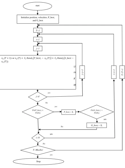
function, the sigmoid function is mapped as much as 0.5. On the other hand, increasing the velocity of the particle in both the positive and negative directions means increasing the probability of changing the position of the particle, so that at the beginning and the end of the interval, the magnitude of the probability function must be equal to one. Therefore, multiplication 2 is used in Eq. (6). Also in proposed method chaos logistic map used to determine the inertia weight that prevents early convergence. So it helps to produce a better quality solution. Flowchart of a proposed search method is in Figure 3.

5.

IMPLEMENTATION AND RESULT

EVALUATION

5.1

Dataset

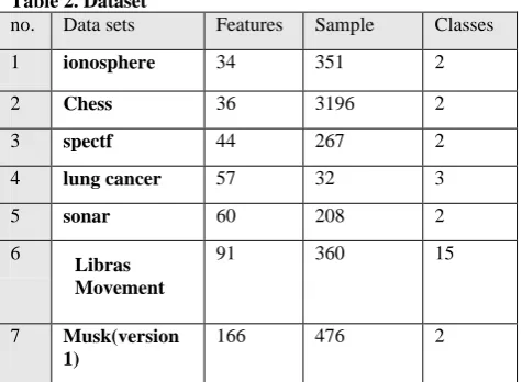
The dataset in this paper is coming from UCI (https://archive.ics.uci.edu/ml/datasets.html). Data sets are selected such that cover medium and large scale of the feature selection problem. Data sets with number of features between 20, 49 are medium scale and greater than 50 are large [50]. Table 2 shows selected data set from UCI and their characteristic.

Table 2. Dataset

no. Data sets Features Sample Classes

1 ionosphere 34 351 2

2 Chess 36 3196 2

3 spectf 44 267 2

4 lung cancer 57 32 3

5 sonar 60 208 2

6

Libras Movement

91 360 15

7 Musk(version 1)

166 476 2

For controlling of domain values of each feature, Features are normal in the range of 0 and 1 (except Libras dataset that are between 0, 1) normalization formula is as follows:

𝑥

= 𝑥− 𝑚𝑖𝑛𝑥

𝑚𝑎𝑥𝑥−𝑚𝑖𝑛𝑥 (9)

In Eq. (9), 𝑥 is the value of feature, minx is minimum and

Fig 4: Flowchart of proposed method

5.2

Initial parameters setting up

CNBPSO such as every version of original BPSO have parameters must be adjusted. This parameter includes number of particles, acceleration constants, inertia weight setting up and stopping criteria. In this application the number of particles is 20, acceleration constants are 1.49, for setting up inertia weight; the start point of logistic map chaotic sequence is 0.86. The stopping criterion of CNBPSO is after 200 iterations. The minimum and maximum velocity are -6 and 6

respectively. This value is almost ubiquitously adopted in PSO research [41].

5.3

Experimental evaluation

In this section, the effectiveness of the proposed method on datasets that introduced in section 5.1. have been evaluated. The proposed model is implemented in MATLAB software and on computer using Intel core i7. Diversity of dataset has been considred; especially in terms of number of features. The

start

i=1

j=1

𝐼𝑓𝑣𝑖𝑗 𝑇 + 1 ∉ 𝑉𝑚𝑖𝑛 , 𝑉𝑚𝑎𝑥

𝑡ℎ𝑒𝑛 𝑣𝑖𝑗 𝑇 + 1 = max 𝑚𝑖𝑛 𝑉𝑚𝑎𝑥, 𝑣𝑖𝑗 𝑇 + 1 , 𝑉𝑚𝑖𝑛

𝑺′ _𝒗

𝒊𝒋 𝑻 + 𝟏 = 𝟐 ∗ 𝒂𝒃𝒔 𝑺 𝒗𝒊𝒋 𝑻 + 𝟏 − 𝟎. 𝟓

𝑰𝒇 𝒓𝒂𝒏𝒅 < 𝑺′_(𝒗

𝒊𝒋 𝑻 + 𝟏 ) 𝒕𝒉𝒆𝒏 𝒙𝒊𝒋 𝑻 + 𝟏 = 𝒄𝒐𝒎𝒑𝒍𝒆𝒎𝒆𝒏𝒕 𝒙𝒊𝒋 𝑻 ;

𝒆𝒍𝒔𝒆 𝒙𝒊𝒅 𝑻 + 𝟏 = 𝒙𝒊𝒅 𝑻

𝑣𝑖𝑗(𝑇 + 1)=𝑤 𝑣𝑖𝑗(𝑇) + 𝐶1 𝑅𝑎𝑛𝑑1 𝑃_𝑏𝑒𝑠𝑡𝑖− 𝑥𝑖𝑗(𝑇) + 𝐶2 𝑅𝑎𝑛𝑑2 𝐺_𝑏𝑒𝑠𝑡 −

𝑥𝑖𝑗(𝑇)

j<d

j=j+

1

yes

No

yes

P_besti = Xi

Fit(G_besti ) <

Fit(Xi)

yes

G_besti = Xi

i<N

T<MaxIter

yes

No

Stop

Fit(P_besti )<

Fit(Xi)

Initialize position, velocities, P_best, and G_best

T=1

yes

i=i+

1

No

T=T+

results of the proposed method (CNBPSO) have been compared with BPSO and CBPSO. All algorithms have the same parameters and used 1-nearest neighbor by leave one out cross validation to select an optimal subset, just only inertia weight for BPSO is constant, namely 0.48. Due to the nature of randomizing of algorithms; we run them ten times and we report average classification accuracy too. Our result adjusts in three tables in terms of average of accuracy, the best accuracy and smallest feature subset between ten times run. As shown in Table 3, the average classification accuracies of the ionsphere, chess, lung cancer, sonar, libras and musk obtained by BPSO are 93.48%,97.66%,83.15%, 75.94%,93.13%,89.58% and 91.74% respectively. the average classification accuracies of the ionsphere, chess, lung cancer, sonar, libras and musk classification problems obtained by CBPSO are 93.82%,97.86%, 83.11%,77.19%,92.98%,89.75% and 91.93% respectively. Also the average classification

accuracies of the ionsphere, chess, lung cancer, sonar, libras and musk classification problems obtained by CNBPSO are 94.04%,98.18%,84.27%,81.87%,94.28%, 90.33% and 94.45% respectively. The results show in Table 3 that in case of average; CNBPSO has better performance (in terms of accuracy) than BPSO and CBPSO to find optimal subset. But this performance is associated with average number offeature increased.

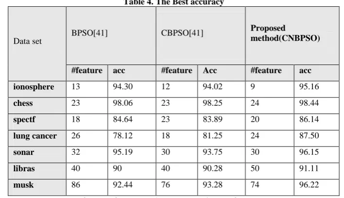
The best obtained accuracy in during oftentimes run of BPSO, CBPSO and CNBPSO shows in Table 4. In terms of the best accuracy, the proposed method has better result (accuracy) than CBPSO and BPSO, but associated with increasing number of features except Ionosphere and Musk. In following the smallest feature subset is coming in Table 5 in during of 10 times run algorithms.

Table 3. Average accuracy

Data set

Without feature

selection BPSO[41] CBPSO[41]

Proposed

method(CNBPSO)

#feature acc #feature acc #feature acc #feature Acc

ionosphere 34 86.89 14.5 93.48 13.2 93.82 12.6 94.04

chess 36 83.76 21.4 97.66 22.9 97.86 22.4 98.18

spectf 44 69.29 22.06 83.15 22.4 83.11 24.22 84.27

lungcancer 57 43.75 28.1 75.94 26.6 77.19 28 81.87

sonar 60 87.5 30 93.13 29.7 92.98 31.6 94.28

libras 91 87.22 42.7 89.58 41.9 89.75 44.4 90.33

musk 166 85.92 81 91.74 85.2 91.93 85.2 94.45

#feature= average of feature numbers, acc=Average of accuracy Table 4. The Best accuracy

Data set

BPSO[41] CBPSO[41] Proposed

method(CNBPSO)

#feature acc #feature Acc #feature acc

ionosphere 13 94.30 12 94.02 9 95.16

chess 23 98.06 23 98.25 24 98.44

spectf 18 84.64 23 83.89 20 86.14

lung cancer 26 78.12 18 81.25 24 87.50

sonar 32 95.19 30 93.75 30 96.15

libras 40 90 40 90.28 50 91.11

musk 86 92.44 76 93.28 74 96.22

Table 5. The smallest feature subset

Data set

BPSO[41] CBPSO[41]

Proposed

method(CNBPSO)

#feature acc #feature acc #feature acc

ionosphere 11 93.45 12 94.02 9 95.19

chess 17 97.62 19 97.78 21 98.25

spectf 18 84.64 15 83.15 20 86.14

lungcancer 22 71.87 18 81.25 22 84.37

sonar 26 93.27 26 93.27 27 95.19

libras 37 89.44 35 90 33 90.83

musk 67 91.81 76 93.28 66 96

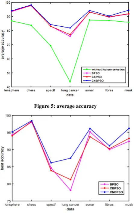
#feature= minimum feature numbers, acc= accuracy To have quick comparison between algorithms, you can see

the results in the Figure 4 and 5. Figure. 4 shows datasets versus average accuracy of each algorithm and Figure. 5 shows datasets versus best accuracy of each algorithm. Y axis is the percent of accuracy and X axis is dataset that used in our paper.

Figure 5: average accuracy

Figure 6: Best accuracy

6.

CONCLUSION

AND FUTURE WORK

Feature selection is an important preprocessing technique in many applications. Due to be intractable of problems, search is a key issue. In this paper, we have presented a new way of wrapper feature selection for classification tasks. The proposed method (CNBPSO) by using new likelihood function and chaotic logistic map for inertia weight; attempt to find the best feature subset such that accuracy of classification increase. In fact with this modification, proposed method avoid falling in local minima and as the results show, produce better result than BPSO and CBPSO. In the future, it is recommended to use multi objective method for feature selection problem and also it is recommended to combine other heuristic method and chaos sequences algorithms for feature selection problem.

7.

REFERENCES

[1] Mitra, S. Kundu, P. and Pedrycz, W. 2012. Feature selection using structural similarity. Information Sciences. 198, 48–61.

[2] Kanan, H. R. and Faez, K. 2008. An improved feature selection method based on ant colony optimization (aco) evaluated on face recognition system. Applied Mathematics and Computation. 205, 716–725.

[3] Wang, Y. Dahnoun, N. and Achim, A. 2012. A novel system for robust lane detection and tracking. Signal Processing. 92, 319–334.

[4] Zhou, H. You, M. Liu, L. Zhuang, C. 2017. Sequential data feature selection for human motion recognition via Markov blanket. Pattern Recognition Letters. 86, 18-25. [5] Mandloi, A. and Gupta, P. 2017. An Effective Modeling

for Face Recognition System: LDA and GMM based Approach. International Journal of Computer Applications. 180(1).

741.

[7] Eisa, D. A. Taloba, A. I. and Ismail, S. S. I. 2018. A comparative study on using principle component analysis with different text classifiers. International Journal of Computer Applications. 180(31).

[8] Jain, A. and Zongker, D. 1997. Feature selection: evaluation, application, and small sample performance. Ieee Transactions on Pattern Analysis and Machine Intelligence. 19, 153 - 158.

[9] Novaković, J. Strbac, P. and Bulatović, D. 2011. Toward optimal feature selection using ranking methods and classification algorithms. Yugoslav Journal of Operations Research. 21(1), 119-135.

[10]Chen, Y. Li, Y. Cheng, X. and Guo, L. 2006. Survey and taxonomy of feature selection algorithms in intrusion detection system. Lecture Notes in Computer Science. 4318, 153-167.

[11]Ferreira, A. J. and Figueiredo, M. A. T. 2012. Efficient feature selection filters for high-dimensional data. Pattern Recognition Letters.33, 1794–1804.

[12]Dash, M. and Liu, H. 1997. Feature selection for classification. Intelligent Data Analysis.1, 131–156. [13] Hall, M. A. 1999. Correlation-based feature selection for

machine learning. Doctoral Thesis. University of Waikato.

[14]Aghdam, H. M. Aghaee, G. N. Basiri, M. E. 2009. Text feature selection using ant colony optimization. Expert Systems with Applications. 36, 6843–6853.

[15]Gheyas, I. A. and Smith, L. S. 2010. Feature subset selection in large dimensionality domains. Pattern Recognition. 43, 5-13.

[16] Hua, J. Tembe, W. and Dougherty, E. R. 2008 Feature selection in the classification of high-dimension data. Ieee International Workshop on Genomic Signal Processing and Statistics.1–2.

[17]Jin, X. Xu, A. Bie, R. and Guo, P. 2006. Machine learning techniques and chi-square feature selection for cancer classification using SAGE gene expression profiles. Lecture Notes in Computer Science. 3916, 106–115.

[18] Liao, C. Li, S. and Luo, Z. 2007. Gene selection using wilcoxon rank sum test and support vector machine for cancer. Lecture Notes in Computer Science. 4456, 57– 66.

[19]Peng, H, Long, F. and Ding, C. 2005. Feature selection based on mutual information criteria of max-dependency, max-relevance, and min redundancy. Ieee Transactions on Pattern Analysis and Machine Intelligence. 27, 1226– 1238.

[20]Biesiada, J. and Duch, W. 2008. Feature selection for high-dimensional data—a pearson redundancy based filter. Advances in Soft Computing. 45, 242–249. [21]Rocchi, L. Chiari, and L. Cappello, A. 2004. Feature

selection of stabilometric parameters based on principal component analysis. Medical and Biological Engineering and Computing. 42, 71–79.

[22]Kira, K. and Rendell, L. A. 1992. The feature selection problem: traditional methods and a new algorithm, In:

Proceedings of Ninth National Conference on Artificial Intelligence. 129–134.

[23]Almuallim, H. and Dietterich, T. G. 1991. Learning with many irrelevant features, In: Proceedings of Ninth National Conference on Artificial Intelligence. 547–552. [24]Liu, H. and Setiono, R. 1996. A probabilistic approach to

feature selection – a filter solution In: Proceedings of Ninth International Conference on Industrial and Engineering Applications of AI and ES. 284–292. [25]Raman, B. and Ioerger, T. R. 2002. Instance based filter

for feature selection. Journal of Machine Learning Research. 1, 1–23.

[26]Jensen, R. and Shen, Q. 2001. A rough set aided system for sorting WWW bookmarks. Web Intelligence: Research and Development. 95–105.

[27]Traina, C. Traina, A. Wu, L. and Faloutsos, C. 2000. Fast feature selection using the fractal dimension, In: Proceedings of the fifteenth Brazilian Symposium on Databases (SBBD). 158–171.

[28] Chen, B. Chen, L. Chen, Y. 2013. Efficient ant colony optimization for image feature selection. Signal Processing 93, 1566–1576.

[29]Peng, H. Long, F. and Ding, C. 2003. Overfitting in making comparisons between variable selection methods. Journal of Machine Learning Research. 3, 1371–1382. [30]Guan, S. Liu, J. and Qi, Y. An incremental approach to

contribution based feature selection. Journal of Intelligence Systems. 13.

[31]Gasca, E. Sanchez, J. S. and Alonso, R. 2006. Eliminating redundancy and irrelevance using a new MLP-based feature selection method. Pattern Recognition. 39, 313–315.

[32] Hsu, C. Huang, H. and Schuschel, D. 2002 The ANNIGMA-wrapper approach to fast feature selection for neural nets. Ieee Transactions on Systems, Man, and Cybernetics – Part B: Cybernetics. 32, 207–212. [33]Kabira, M. M. Shahjahan, M. and Murase, K. 2012. A

new hybrid ant colony optimization algorithm for feature selection. Expert Systems with Applications. 39, 3747– 3763.

[34]Sivagaminathan, R. K. and Ramakrishnan, S. A. 2007. Hybrid approach for feature subset selection using neural networks and ant colony optimization. Expert Systems with Applications. 33, 49–60.

[35]Tsai, C. F. Eberle, W. and Chu, C. Y. 2013. Genetic algorithms in feature and instance selection. Knowledge Based Systems. 39, 240-247.

[36] Yang, W. Li, D. and Zhu, L. 2011. An improved genetic algorithm for optimal feature subset selection from multi-character feature set. Expert Systems with Applications. 38, 2733–2740.

[37] Sahu, B. Mishra, D. A. 2012. Novel feature selection algorithm using particle swarm optimization for cancer microarray data. Procedia Engineering. 38, 27-31. [38]Wang, X. Yang, J. Teng, X. Xia, W. and Jensen, R.

[39]Kennedy, J. and Eberhart, R. C. 1995. Particle swarm optimization. In: Proceedings of the Ieee International Conference on Neural Networks. 4, 1942–1948.

[40]Thangavel, K. Bagyamani, J. Rathipriya, R. 2012. Novel hybrid pso-sa model for biclustering of expression data. Procedia Engineering. 30, 1048 – 1055.

[41]Chuang, L. Yang, C. and Li, J. C. 2011. Chaotic maps based on binary particle swarm optimization for feature selection. Applied Soft Computing. 11, 239–248. [42]Kennedy, J. and Eberhart, R. C. 1997. A discrete binary

version of the particle swarm algorithm. In: Proceedings of the 1997 Conference on Systems, Man, and Cybernetics. 4104–4109.

[43] Unler, A. Murat, A. 2010. A discrete particle swarm optimization method for feature selection in binary classification problems. European Journal of Operational Research. 206, 528–539.

[44]Rostami, N. and Nezamabadi, H. 2006. A new method for binary PSO. In: proceedings of the international Conference on Electronic Engineering (in Persian). [45]Nickabadi, A. Ebadzadeh, M. M. and Safabakhsh, R.

2011. A novel particle swarm optimization algorithm with adaptive inertia weight. Applied Soft Computing. 11, 3658–3670.

[46]Shen, Yi. Bu, Y. Yuan, M. 2009. A novel chaos particle swarm optimization (pso) and its application in pavement maintance decision. In: Proceedings on Fourth Ieee Conference on Industrial Electronics and Applications. 3521-3526.

[47] Chuang, L. Y. Hsiao, C. J. and Yang, C. H. 2011. Chaotic particle swarm optimization for data clustering, Expert Systems with Applications. 38, 14555–14563. [48]Jiang, L. Cai, Z. Wang, D. and Jiang, S. 2007. Survey of

improving k-nearest-neighbor for classification. In: Proceedings of Fourth International Conference on Fuzzy Systems and Knowledge Discovery . 1, 679 – 683.

[49]Wu, X. et al. 2008. Top 10 algorithms in data mining. Knowl Inf Syst. 14, 1–37.