Essays in international monetary economics

(1)

University of Warwick institutional repository: http://go.warwick.ac.uk/wrap

A Thesis Submitted for the Degree of PhD at the University of Warwick

http://go.warwick.ac.uk/wrap/2806

This thesis is made available online and is protected by original copyright. Please scroll down to view the document itself.

(2)

Essays in International Monetary Economics

Christian Saborowski

A Thesis submitted for the degree of Doctor of Philosophy

Department of Economics

University of Warwick

(3)

List of Figures

2.1 Post-Disinflation Path of the New Wage . . . 21

2.2 Closed Economy: Post-Disinflation Path with Oscillations . . 29

2.3 Closed Economy: Post-Disinflation Path without Oscillations . 31 3.1 Open Economy: Post-Disinflation Path with Oscillations . . . 43

3.2 Open Economy: Post-Disinflation Path without Oscillations . 44 3.3 The Effect of the Inflation Rate on Output . . . 48

3.4 Comparison of the Linear and the Nonlinear Model I . . . 61

3.5 Comparison of the Linear and the Nonlinear Model II . . . 62

3.6 Nonlinear Model: Partial Disinflation with Oscillations . . . . 63

3.7 Nonlinear Model: Partial Disinflation without Oscillations . . 64

5.1 Benchmark Specification . . . 128

5.2 Benchmark Specification: Different Types of Capital Flows . . 132

A.1 Case 1: Unstable Pattern . . . 176

A.2 Case 2: Stable Pattern . . . 177

A.3 Smoothed Unconditional Probability of Being in the Informed Trading State - Comparison Between Different Types of Days 194 A.4 Smoothed Unconditional Probability of Being in the Informed Trading State on MPC Days with Surprise Announcements -Different Surprise Measures . . . 195

A.5 Decomposition of Net Capital Flows to the United States (in billions of USD) . . . 196

A.6 Robustness Exercise: Fry and Pagan (2007) Critique . . . 198

A.7 Equity Parity and Implied Sharpe Ratio . . . 199

A.8 Robustness Exercise: No Restriction on Consumption . . . 200

A.9 Robustness Exercise: No Restriction on Consumption - Dif-ferent Types of Capital Flows . . . 201

A.10 Robustness Exercise - Identifying Multiple Shocks . . . 202

(6)

(7)

List of Tables

3.1 Maximum Value ofµI Allowing the Policymaker to Avoid the

Liquidity Trap . . . 55

3.2 Nontradables Output for Different Calibrations . . . 57

4.1 GARCH Model of Daily Exchange Rate Returns . . . 86

4.2 Constant Transition Probability Model . . . 88

4.3 Preferred Time-Varying Transition Probability Model . . . 89

4.4 Markov Switching Model Including Additional Constant Terms 91 4.5 Additional Variables Added to the Preferred Model Specification 93 4.6 Controlling for ECB Monetary Policy Announcements . . . 95

4.7 Markov-Switching Model of MPC News Anticipation Effects . 97 4.8 Markov-Switching Model Taking Account of Forecast Dispersion101 5.1 Sign Restrictions . . . 121

5.2 Variance Decomposition . . . 139

5.3 Variance Decomposition: Fry and Pagan (2007) . . . 139

A.1 The Welfare Effects of the Disinflation Policy for Different Calibrations . . . 184

A.2 Monetary Policy Committee Meetings, Interest Decisions and Surprise Measures I . . . 187

A.3 Monetary Policy Committee Meetings, Interest Decisions and Surprise Measures II . . . 188

A.4 Monetary Policy Committee Meetings, Interest Decisions and Surprise Measures III . . . 189

A.5 GARCH Model: Surprise if Change in 3 Months Interbank Rate is Greater Than 9 . . . 190

A.6 GARCH Model: Surprise if Change in 3 Months Interbank Rate is Greater Than 14 . . . 190

(8)

A.8 GARCH Model: Surprise if Change in Price of 3 Months In-terest Rate Futures is Greater Than 14 . . . 191 A.9 MS Model: Surprise if Change in 3 Months Interbank Rate is

Greater Than 9 . . . 192 A.10 MS Model: Surprise if Change in 3 Months Interbank Rate is

Greater Than 14 . . . 192 A.11 MS Model: Surprise if Change in Price of 3 Months Interest

Rate Futures is Greater Than 9 . . . 193 A.12 MS Model: Surprise if Change in Price of 3 Months Interest

(9)

Acknowledgements

(10)

Abstract

Chapter 2 of this thesis employs a dynamic general equilibrium with Tay-lor wage contracts to show that the use of strict inflation targeting as a disinflation policy may result in a slump in production and a considerable increase in macroeconomic volatility. Important determinants of the magni-tude of the macroeconomic oscillations in the post-disinflation state of the economy turn out to be the size of the reduction in the inflation rate and the degree of returns to labor in the production function. In the special case of constant returns, the oscillations are large and permanent.

Chapter 3 of this thesis extends the above analysis to an open-economy setting demonstrating that the exchange rate can act as a stabilizer by effec-tively relieving wages from part of the burden of reducing the inflation rate. The more the economy is open, the smaller the magnitude of the macroeco-nomic oscillations will be after the disinflation policy is applied. The policy is shown to be infeasible for all practical purposes in a closed economy with constant returns to scale when the full nonlinear model is considered.

Chapter 4 of this thesis employs a Markov switching framework to allow for an interesting alternative characterization of macroeconomic news effects on the foreign exchange market. The chapter finds strong evidence for the presence of nonlinear regime switching between a high-volatility and a low-volatility state driven by monetary policy announcements that come as a surprise to the market. It also uncovers significant market positioning prior to the announcements, indicating a limiting of risk exposure by market par-ticipants who are unsure about the precise outcome of the policy decisions.

(11)

Chapter 1 Introduction

A growing number of both theoretical and applied economists have devoted

their time to the study of the conduct of monetary policy in recent years.

Two developments stand out as factors increasing this interest.

First and foremost, progress in macroeconomic theory has been

remark-able, with a new generation of quantitative models developed under the New

Keynesian paradigm that can be used to explicitly study the impact of

sta-bilization policies on economic welfare. Perhaps most importantly, these

models can claim sufficient realism to be of interest to policymakers around

the globe (Woodford, 2006). The origin of this influential literature lies in

the synthesis of two independent theories of macroeconomic modelling. In

particular, it is grounded in the idea to enrich real business cycle models

of dynamic individual optimization (Prescott, 1986) with Keynesian

con-cepts such as nominal price rigidity and the inefficiency of aggregate

fluc-tuations. The latter had previously been developed in static models

(12)

and Romer, 1991). The development of tightly structured macroeconomic

models based on explicit theoretical microfoundations and capable of

suc-cessfully capturing macroeconomic time series data (Christiano, Eichenbaum

and Evans, 2005; Smets and Wouters, 2003) have led to a comeback of the

quantitative assessment of the optimal conduct of monetary policy (Gali,

2007).

The second reason for the popularity of the field is progress in the

pro-fession of central banking itself. A growing number of central banks have

come to organize monetary policy around an explicit set of objectives. One

way of specifying such objectives is via an explicit inflation forecast

target-ing rule as, for example, followed by the Reserve Bank of New Zealand and

the Bank of England. Increased efforts to communicate policy goals to the

general public also emphasize the importance of a clear framework to guide

policy decisions (Woodford, 2006). In the light of these facts, it has become

increasingly common to use structural macroeconomic models in

policymak-ing institutions around the globe. These developments not only point to the

success of the newly developed quantitative models but also illustrate how

far the profession has come from initial efforts to organize monetary policy

on an almost entirely informal basis.

The optimality of price stability as an objective for monetary policy has

been at the core of this renewed interest in the study of its conduct. As

demonstrated in Woodford (2003) among others, the presence of inflation not

only signals an inefficient level of economic activity but also incurs a more

direct cost by leading to an inefficient allocation of resources and suboptimal

(13)

this result holds in a broad class of sticky price dynamic general equilibrium

(DSGE) models (Christiano, Eichenbaum and Evans, 2005; Gali and Gertler,

1999; Woodford, 1999). At the same time, it is important to notice that there

are good arguments in favour of stabilizing inflation at a strictly positive rate

(e.g. in order to avoid the zero lower bound on nominal interest rates) and at

the medium-term horizon (Gali, 2008). For example, Svensson (2000) shows

that strict inflation targeting, a policy tolerating only minor deviations from

target, leads to substantially more output volatility than a more flexible rule

that targets inflation at a longer horizon.

Chapter 2 of this study somewhat reinforces this result by showing that

the sub-optimality of strict inflation targeting may be even more severe when

the policy is adopted as a disinflation policy, i.e. if it is applied to reduce

the prevailing inflation rate to a lower level.1 _{The chapter is motivated}

by the idea that inflation targeting differs from other disinflation policies in

important respects. In particular, a strict interpretation of an inflation target

allows the policymaker to tolerate only minor deviations from target. But

adjusting the policy instrument such that the inflation rate is reduced to a

new target and defending this target rigorously must preserve inflationary

distortions such as wage and price differentials to an exceptional degree (see

also Yun, 2005). The chapter employs a dynamic general equilibrium with

Taylor wage contracts to show that the use of strict inflation targeting as a

1

(14)

disinflation policy may result in a slump in output and a considerable increase

in macroeconomic volatility. Important determinants of the magnitude of

the macroeconomic oscillations in the post-disinflation state turn out to be

the size of the reduction in the inflation rate and the degree of returns to

labour. In Chapter 3, the analysis is extended to an open-economy setting

demonstrating that the exchange rate can act as a stabilizer by effectively

relieving wages from part of the burden of reducing the inflation rate. The

more the economy is open, the smaller the magnitude of the macroeconomic

oscillations will be after the disinflation policy is applied.

A key merit of an inflation targeting regime under price stability is that

it is believed to successfully anchor private sector expectations. Dating back

to the rational expectations revolution, it is a well-accepted belief that

man-aging private sector expectations successfully is crucial for the optimal

func-tioning of the monetary transmission mechanism. From a macro modeling

perspective, the reason is that current values of aggregate output and

infla-tion depend not only on the central bank’s current choice of the short-term

interest rate, but also on the anticipated future path of this instrument (see

Woodford, 2003). The practical implication is that the central bank’s ability

to manage private sector expectations about its future policy settings has

important consequences for its overall effectiveness. Partially on the grounds

of this understanding, an extensive literature developed that investigates the

role of central bank communication in managing expectations (see Blinder et

al (2008) for an excellent survey). The reaction of asset prices to monetary

policy announcements and communication can not only be an important

(15)

insights about the microstructure of the respective financial markets (see

Sarno and Taylor, 2003).

Chapter 4 of this thesis contributes to this literature by employing a

Markov switching framework in order to allow for an alternative

characteri-zation of macroeconomic news effects on the foreign exchange market. The

underlying hypothesis for the choice of the model is that monetary policy

announcements do not simply affect the market as shocks to an otherwise

continuous process. On the contrary, news effects may change the entire data

generating process underlying a market’s dynamics. An econometric

speci-fication allowing for regime switches therefore appears appropriate. Indeed,

one particular benefit of applying such a model is that it facilitates a

plausi-ble interpretation of observed nonlinearities. In this chapter, we find strong

evidence for nonlinear regime switching between a high-volatility ”informed

trading” state and a low-volatility ”liquidity trading” state driven by

mone-tary policy announcements that come as a surprise to the market. We also

uncover significant market positioning prior to the announcement, indicating

a limiting of risk exposure by market participants.

In Chapter 5, this thesis continues to analyze the impact of monetary

pol-icy on financial markets but returns to the macro perspective. The chapter

investigates the impact of monetary shocks on the direction and the

compo-sition of international capital flows. It employs a standard structural VAR

specification to identify monetary policy shocks, relying on sign restrictions

imposed on the impulse response functions of a few macroeconomic variables,

following closely Canova and De Nicolo (2002) and Uhlig (2005). The

(16)

a statistically and economically meaningful effect on US capital flows and

the trade balance. An exogenous easing of US monetary policy by 100 basis

points induces net capital inflows and a worsening of the US trade balance

of around 1% of GDP after 8 quarters. The second main result focuses on

the effect of monetary policy shocks on the composition of US capital flows.

Intriguingly, it is found that an exogenous US monetary policy easing causes

net inflows in debt securities, foreign direct investment (FDI) and other

in-vestment, while inducing net outflows in portfolio equities from the United

States. Monetary policy shocks thus entail a conditional negative

correla-tion between flows in portfolio equity and debt. A key for understanding

this conditional correlation is the effect of monetary policy shocks on asset

prices. While a monetary policy easing implies a decrease in short-term (and

long-term) interest rates, it also causes the above mentioned increase in

rel-ative equity returns. Overall, our evidence suggests that monetary policy

shocks induce negative conditional correlations between flows in bonds and

equity securities. Moreover, they cause a negative conditional correlation

be-tween equity flows and equity returns and a positive conditional correlation

(17)

Chapter 2 Strict Inflation Targeting as a

Means of Achieving

Disinflation: A Basic Analysis

2.1 Introduction

Inflation targeting has become increasingly popular as a monetary policy

regime. A distinctive feature of many emerging market economies among

the inflation targeters regards the level of the inflation rate exhibited at the

time of adoption of the policy. Industrial countries have adopted inflation

targeting at inflation rates at least broadly consistent with price stability.

In contrast, emerging market economies such as Mexico, Hungary or Poland

exhibited initial inflation rates of around 10 percent or more.1 _{This study} 1

(18)

is concerned with the macroeconomic effects of the explicit use of inflation

targeting as a disinflation regime. The argument I make is that a strict

inflation targeting policy employed for the purpose of disinflation may

pre-serve inflationary distortions to an unusually large degree. In the model I

employ, these excess distortions not only cause slumps in real activity, but

may additionally increase macroeconomic volatility.

An extensive literature has analyzed inflation targeting with regard to

its properties as a monetary policy regime under price stability. Its

ad-vantages have been documented by, among others, Bernanke and Mishkin

(1997), Svensson (1997) and Svensson and Woodford (2003). In an early

contribution, Svensson (2000) differentiates between flexible and strict

infla-tion targeting and shows that the former creates substantially less output

variability than a strict interpretation of the policy, as it effectively targets

inflation at a longer horizon. The present paper somewhat reinforces this

result by showing that the sub-optimality of strict inflation targeting may be

even more severe in the context of a disinflation episode. Yun (2005) applies

a similar line of reasoning as I do in this paper. He shows that the zero

inflation optimality result (Woodford, 1999; Gali, 2000) must be refined in

the presence of initial price dispersion.2 _{The reason is that the pre-existing}

price dispersion adversely affects real activity in the economy and converges

2

(19)

faster under alternative policies.3

The literature on the real effects of disinflations has concentrated on

ex-plaining stylized facts regarding the differential real effects of money- and

exchange-rate-based disinflations. Among others, Ball (1994) and Ascari and

Rankin (2002) consider explanations for the finding that money-based

dis-inflations typically cause slumps in output on impact. Exchange-rate-based

policies, on the other hand, are frequently characterized by initial booms

in real activity. Calvo and Vegh (1994) replicate this empirical finding by

assuming that a collapse of the disinflation policy is rationally anticipated.

Fender and Rankin (2007) explain the boom with an element of

preannounce-ment of the policy under a standard type of exchange rate peg.4 _{The long run}

impact of disinflation policies in the framework of the New Keynesian model

is discussed in Blanchard and Gali (2007) and Ascari and Merkl (2007). The

present study is motivated by the idea that inflation targeting differs from

other disinflation policies in important respects. In particular, a strict

inter-pretation of an inflation target allows the policymaker to tolerate only minor

deviations from target. But adjusting the policy instrument such that the

inflation rate is reduced to a new target and defending this target rigorously

must preserve inflationary distortions such as wage and price differentials to

an exceptional degree.

In this chapter, I use a Dynamic General Equilibrium Model with wage

staggering of the type suggested by Taylor (1979a) to consider a rather

ex-3

The stabilization policy examined in Yun (2005) does not increase macroeconomic volatility. The reason is that the author uses Calvo (1983) price contracts. I elaborate on this below.

4

(20)

treme case of a disinflation exercise: an immediate and permanent reduction

in the rate of CPI inflation to a newly set target. I interpret this policy as

strict inflation targeting during a disinflation episode. The central bank sets

the path of money supply such that the newly set inflation target is attained

immediately and sustained throughout future periods. The particular nature

of the policy requires me to solve the model in a rather unconventional way.

I first impose the result of the disinflation policy, a reduction to a lower rate

of CPI inflation, and then solve for the policy itself, i.e. the path that money

supply has to follow in order to sustain the new inflation target throughout

the future.

I begin by considering a closed economy version of the model. As briefly

mentioned above, I find that the disinflation policy I consider not only

cre-ates a slump in output on impact, but can additionally generate oscillatory

behavior in both nominal and real variables along their post-disinflation

ad-justment paths. The reason is that the immediate reduction in price inflation

requires the real wage to fluctuate for some periods before it gradually

con-verges to its new steady state. The oscillations can be permanent when the

returns to labor in the production function are constant. From a modeling

perspective, the presence of oscillations along the adjustment path is a result

that would not obtain in a model with a Calvo (1983) type staggering

struc-ture. I show that this is because price setters in such a model would always

set prices equal to the prevailing price level. In the framework of model used

in this study, I distinguish two cases: one in which the economy is indeed

characterized by oscillatory behavior along its post-disinflation path and one

(21)

the size of the initial slowdown in real activity is strongly positively related

to the presence of oscillations along the adjustment path.

The presence and the magnitude of oscillations along the economy’s

ad-justment path naturally depend on the degree to which wages need to

fluc-tuate in order to keep the inflation rate at the newly set target. Important

determinants are thus the desired size of the reduction in the inflation rate

as well as the returns to labor in the production function. Greater returns

to scale generate oscillations as they imply that wages are tied more closely

to the behavior of prices. In particular, I find that there are no oscillations

at all along the post-disinflation path of the economy if the returns to labor

are sufficiently low. At the other extreme, in the case of constant returns to

scale, the oscillations are large and permanent. The latter is thus the only

case in which the economy does not gradually converge to a new steady state.

The rest of the chapter is organized as follows. Section 2.2 outlines the

structure of the model. Section 2.3 examines the implications of the

disinfla-tion policy and highlights the degree of returns to scale as a decisive factor in

determining the magnitude of the oscillations in the post-disinflation state.

Section 2.4 concludes.

2.2 The Model Economy

In this section, I employ a closed economy Dynamic General Equilibrium

Model with imperfect competition in the labor market and nominal wage

rigidities of the type proposed by Taylor (1979). The structure of the model

(22)

and to derive crucial results analytically. I omit derivations where they are

standard in the literature.

The economy is inhabited by a continuum of householdsjǫ[0,1] and firms. The supply side of the economy produces a single consumption good using a

technology in which labor is the only variable factor of production

Yt =Ntσ (2.1)

where Yt is output at time t, σ is the degree of returns to labor and

0 < σ _≤ 1. A typical firm demands a continuum of labor types jǫ[0,1] to minimize the cost of achieving a particular composite labor input Nt, given

by Nt = [

R1 0 L

(ε−₁₎_/ε

jt dj]ε/(ε

−1)

. Ljt is the quantity of labor that household

j supplies to the firm and ε > 1 is the elasticity of technical substitution across labor types. Solving the cost minimization problem yields the standard

conditional demand for labor function

Ljt=Nt(

Wt

Wjt

)ε (2.2)

where Wt is the wage index given by Wt = [R₀1Wjt1−εdj]1/(1

−ε)

. Goods

markets are perfectly competitive. The firm’s profit maximization problem

thus yields the supply function

Yt=Nt(

Wt

σPt

)σ/(σ−1)

(2.3)

I now move to the demand side of the economy. Household j supplies labor

(23)

of two sectors of households. Sector A comprises labor types [0,0.5) and sector B comprises labor types [0.5,1]. Although households are monopolistic suppliers of their individual type of labor input, they are price takers in all

other markets. I assume that they are completely symmetric in terms of their

preference structure which implies that consumption must be equal across

households in a given sector at any point in time. I also assume the existence

of complete domestic asset markets. This implies that households can insure

against any type of initial shock that might affect the two sectors differently

due to the staggering structure to be defined below. Hence, Cjt =Ckt must

hold for any two households j and k in sectors A and B. Finally, I define

aggregate nominal consumption as St = PtCt where Pt is the price of one

unit of the composite consumption good.

Wages are set by each individual household subject to a staggering

struc-ture of the type proposed by Taylor (1979). In particular, I assume that

households in sector A (B) set their wage in even (odd) periods and keep it

fixed for the subsequent period. The wage newly set in period t is denoted

by Xt independently of the sector in which it is set. Households are utility

maximizers. A representative household j in sector A derives utility from

consumption, liquidity holdings and leisure and maximizes her discounted

lifetime utility Uj by choosing a pattern for personal consumption Cjt, bond

holdingsBjt, wagesWjtand labor effortNjtsubject to a series of budget

con-straints, the conditional demand for labor and the wage setting constraint:

Uj =

∞ X

t=0

(24)

subject to

Mjt−₁+I_t−₁B_jt−₁+W_jtL_jt+ Π_t+G_t =P_tC_jt+M_jt+B_jt (2.5)

Ljt=Nt(

Wt

Wjt

)ε (2.6)

Wjt =Wjt+1 =Xt, t= 0,2,4, ... (2.7)

where only the first two constraints must hold in even and odd periods

t = 0,1,2,3, ...and whereβ <1, ζ_≥1,It is the domestic gross interest rate,

Mtdenotes money supply in period t,Gtis a lump-sum subsidy to households

and Πt denotes a share in firms’ profits that is equal across households.5

The optimization problem for household k in sector B is exactly equivalent

except that the wage setting constraint holds in odd instead of even periods.

The first order conditions of this optimization problem are given by the

consumption Euler equation, the money demand optimality condition and

the optimal wage setting condition

Cjt+1 =β[It

Pt

Pt+1

]Cjt (2.8)

Mjt

Pt

=Cjt

1₋δ δ

It

It−1

(2.9)

5

(25)

Xt= [

ε ε₋1

ηζ δ

Lζ_jt+βLζ_jt₊₁

Ljt

PtCjt +β

Ljt+1

Pt+1Cjt+1

] (2.10)

The economy further comprises a government that controls money supply.

Its budget constraint is given by

Gt=Mt−Mt−₁ (2.11)

The competitive equilibrium in the model economy is the sequence of

prices [Xjt, Pt]∞t=0 and allocations [Yt, Cjt, Njt, Ljt, Bjt, Mjt]∞t=0 such that firms

maximize profits, agents maximize utility and all markets clear.6 _{I aggregate}

the equilibrium conditions across individuals and take a log-linear

approxi-mation around a reference steady state in which inflation is zero. Notice that

in what follows I will distinguish between the reference zero inflation steady

state (ZISS) around which the equilibrium conditions are linearized and a

constant inflation steady state (CISS) in which the economy finds itself one

period before the disinflation policy is applied. As the economy is closed,

bond holdings are zero in both states.7 _{The linearized equilibrium}

condi-tions are presented in Appendix A.1.1.8 _{In the following, lower-case symbols}

denote log deviations of variables from their reference steady state values,

i.e. vt=log_VV_Rt.

6

Due to the staggering structure in wages the labor market does not clear in the Wal-rasian sense.

7

While this must necessarily be the case in a closed economy setting, I will impose it upon the open economy by assumption in the next section

8

(26)

2.3 Strict Inflation Targeting as a

Disinfla-tion Policy

I now proceed to assess the macroeconomic effects of a disinflation policy

that uses strict inflation targeting to reduce the rate of CPI inflation from

a positive to a non-negative value. I define strict inflation targeting

follow-ing Svensson (2000). The definition implies that the policymaker only cares

about stabilizing inflation at a given target. I assume that she has perfect

control over the inflation rate and adjusts her policy instrument such that

inflation is kept at target at any point in time. The economy is initially in

a constant inflation steady state (CISS) in which real variables are constant

and all nominal variables grow at some constant inflation rate µI. The

poli-cymaker decides to reduce inflation in periodt= 0 from its initial rateµI to

the lower but nonnegative value µD. This policy change is unexpected and

credible. The policymaker takes action by announcing µD as the new target

and adjusts the path of money supply such that the new target is attained

immediately and sustained throughout future periods.9

There is no doubt that this disinflation policy is more rigid than policies

applied in the real world. However, I present this extreme example as a

benchmark case that allows for an analytical characterization of possible

ad-verse effects of applying a too rigid inflation targeting policy for the purpose

of disinflation. The definition of the policy requires us to solve the model in a

rather unconventional way. I first impose the result of the disinflation policy,

9

(27)

a reduction in the rate of inflation fromµI toµD, and then solve for the path

that the money supply needs to follow in order to achieve and sustain the

newly set inflation target. Finally, I assess the macroeconomic effects of the

disinflation policy.

2.3.1 The Initial Constant Inflation Steady State

Before I can investigate the macroeconomic impact of the disinflation policy,

I need to solve for the equilibrium of the model in the initial CISS. I use the

fact that the new wage xt is homogeneous of degree one in nominal variables

and, when normalized by money supply such that vt= xt−mt, is constant

over time at

v =₋ 1 2γ

−γ1 +β

1₋β +

1₋β

1 +β

µI (2.12)

with γ = ₁₊_ε₍ζ_ζ−1). The CISS value of nontradables output is then given

by

y= σ(1−β)

2(1 +β)γµI (2.13)

We observe that nontradables output is affected positively by the inflation

rate in the CISS. The effect is due to wage setters discounting future utility.

I will further discuss this effect in the next chapter in the context of the full

nonlinear model. In the CISS, all nominal variables grow at the rate µI.

Defining m−₁ as the level of money supply one period before the disinflation

(28)

w−₁=−

1 2

−2β

1₋β +

1₋β

(1 +β)γ

µI+m−₁ (2.14)

Equations (2.13) and (2.14) constitute the CISS solution of the model

one period before disinflation.

The next step in the analysis is to understand, how changes in the rate of

price inflation affect the rest of the economy and in particular the staggered

variable, wages. The supply function (A.5) allows me to write the price index

as a function of output and the wage index

pt =

1₋σ

σ yt+wt (2.15)

The equation illustrates that a given change in the price level is

accommo-dated partly by a reaction of wages and partly by firms adjusting production.

The wage level’s share in facilitating the price change depends positively on

the degree of returns to labor. The reason is that a larger σ implies a less strongly upward sloping marginal cost curve and thus a weaker response of

prices to changes in the level of production in the economy. When σ = 1, the marginal cost curve is horizontal, leaving no role for output in the

deter-mination of prices. This implies that the wage level must move one for one

with the price index. In the context of our disinflation policy the latter case

corresponds to a situation in which a reduction in the rate of price inflation

translates one for one into a reduction in the growth rate of the wage

in-dex. The subsequent section will show that this property allows for a purely

(29)

2.3.2 The Special Case: Constant Returns to Scale

I begin by solving for the impact of the disinflation policy in the special

case of constant returns to scale. I do so because the distinctive implications

of this assumption allow for a good understanding of the channels through

which the policy affects the economy.

As a starting point, it is important to notice that there is a crucial

im-plication arising from the assumption of constant returns to scale in the

production function. In particular, equation (A.5) shows that this is the one

and only case for which it is not possible to solve for output when the paths

of both the wage index and the price level are known. The reason is that the

aggregate supply curve, i.e. the relationship between output and the price

level, is horizontal for a given wage. This implies that conventional solution

techniques cannot be applied to determine the full post-disinflation solution

of the model, a point that will perhaps become more obvious when I examine

the general case of σ <1 in the next section.

There is, however, another anomaly about the case of constant returns to

scale. In the previous subsection I have shown that σ = 1 implies that the wage index moves one for one with the price index and a policy of reducing

CPI inflation effectively becomes one of reducing the growth rate of the wage

index. Using this fact, it turns out to be possible to directly solve for the

post-disinflation path of the real side of the economy by distinguishing the

economy’s law of motion in even periods from the law of motion in odd

periods. To see this, remember that our disinflation policy reduces CPI

(30)

that the wage index moves one for one with prices, it is easy to see what such

a policy implies for the behavior of sectoral wages. I take the wage index

and its one period lag. I evaluate the difference at t= 0. This yields

w0−w−₁ =

1

2(x0−x−1) + 1

2(x−1−x−2) (2.16) I have assumed that the economy is in a CISS up until period t = 0. It follows that the second term on the RHS is predetermined and equal to 1

2µI.

Reducing inflation to µD in periodt= 0 then implies that the LHS of (2.16)

is equal to µD. Hence,

x0−x−₁ = 2µ_D−µ_I (2.17)

Following the equivalent procedure for the subsequent periods, we have

xt−xt−₁ = 2µ_D −µ_I (2.18)

for all t= 0,2,4, . . . ,_∞, and

xt−xt−₁ =µ_I (2.19)

for allt= 1,3,5, . . . ,_∞. In other words, wages grow at the constant rate 2µD from one even period to the other and from one odd period to the other.

But, since µD < µI the new wage grows faster from even to odd periods than

from odd to even periods. Three cases are possible. First, if 2µD < µI, the

new wage set in even periods is lower than the wage set in the previous odd

(31)

[image:31.612.148.451.74.323.2]

Figure 2.1: Post-Disinflation Path of the New Wage

the post-disinflation state. Second, if 2µD > µI, the new wage set in even

periods is higher than the wage set in the previous odd period. Third, if

2µD = µI, the new wage set in even periods is equal to the prevailing one

from the previous odd period.

Figure 2.1 illustrates these three cases. The special case of µD = 0 is

represented by Case 1b. It represents a complete disinflation, i.e. a reduction

in the rate of wage inflation from µI to zero. In particular, µD = 0 implies

that

x−2 =x0 =x2 =...=w−1−

1

(32)

x−₁ =x₁ =x₃ =...=w−₁+

1

2µI (2.21)

That is to say that the disinflation policy produces a wage gap between

the two sectors of households that is constant and permanent. The intuition

is the following: I imposed zero wage inflation from period zero onwards. The

wage set in period t=₋2 is smaller than the one set in periodt=₋1. This implies that the wage index requires downward pressure by the new wage set

in period zero to ensure zero wage inflation. Due to the fact that the wage

index is an equally weighted average of the two sectoral wages, the necessary

amount of downward pressure is achieved if the wage in period t = 0 is set equal to wage set in period t = ₋2. The opposite reasoning applies in the subsequent period.

Let us get back to the more general case of an inflation reduction from a

constant value µI to a lower positive value µD. Having determined the wage

setting behavior of households after the disinflation policy is introduced, I can

now derive the entire post disinflation state of the economy. We substitute

for both the wage index and employment in the wage setting condition (A.6)

and obtain

xt=

1 1 +β

st

2γ

1 +γ +xt−1

1₋γ

1 +γ

+ β

1 +β

st+1

2γ

1 +γ +xt+1

1₋γ

1 +γ

(33)

We already know how wages behave in the post-disinflation state of the

economy. In principle, we can simply impose their paths on the law of motion

of the economy. However, it is important to notice that the dynamic path

of sectoral wages differs between even and odd periods. This implies that

we have to look at each period separately. Using the wage setting condition

(A.6) and substituting from equations (2.20) and (2.21), we have that

st+

1

βst−1 =

1 +β

β (w−1+

1

2µI+tµD)− 1₋γ

2γ (2µD−

1 +β

β µI) (2.23)

st+

1

βst−1 =

1 +β

β (w−1−

1

2µI+ (t+ 1)µD)− 1₋γ

2γ (

1 +β β µI−

1

β2µD) (2.24)

in odd and even periods respectively. These relationships hold from period

zero onwards. A similar relationship betweens0 ands−1would be convenient

as it would uniquely determine the post disinflation path of st. However,

the equivalent procedure would give us a relationship between s−1 and the

expectation of s0 as of period t =−1. And this expectation is false as soon

as the disinflation policy is introduced. The reason is that, in periodt =₋1, the wage setter does, by assumption, not know that the disinflation policy

(34)

out to be different from her expectation as of periodt =₋1. But we can get around this problem by appealing to stability reasoning. From (2.23) and

(2.24), we have that in odd and even periods respectively

st+2−

1

β2st=µD

β2₋₁

β2 t+

β2₋₁

β2 w−₁−µ_I(

1 +β β )

2 1

2γ +µD(3 +

2β₋γ β2_γ )

(2.25)

st+2−

1

β2st=µD

β2₋₁

β2 t+

β2 ₋₁

β2 w−1+µI(

1 +β β )

2 1

2γ +µD(3−

γ+ 1 +β2

β2_γ )

(2.26)

Equations (2.25) and (2.26) are the basic laws of motion of the economy in

the post disinflation state. In order to arrive at a stationary solution, I deflate

both difference equations by the wage level wt. I create a new variable at

defined as the ratioat =st−wt. The resulting first order difference equations

in at take the form

at+2 =

1

β2at+constant (2.27)

Since β < 1, the Eigenvalue of these equations is greater than one and unstable. This implies that there is a unique non divergent solution for each

of these processes as Blanchard and Kahn (1980) show. This non divergent

solution obtains when at is equal across odd and across even periods. The

economy instantly jumps to its post disinflation state and remains there.

(35)

yodd=

(1 +β) 2(1₋β)γµI−

2β

(1₋β2₎_γµD (2.28)

yeven =−

(1 +β) 2(1₋β)γµI+

(1 +β2)

(1₋β2₎_γµD (2.29)

As is evident from equations (2.28) and (2.29), the disinflation policy

re-sults in output oscillations between even and odd periods. The amplitude

of these oscillations is constant. Moreover, we can observe that the extent

to which nominal and real variables fluctuate depends positively on the

ini-tial inflation rate and negatively on the post-disinflation rate. The reason

is that the inflation rate determines the degree of wage dispersion present

in the initial CISS. This suggests that a more gradual path of disinflation

may attenuate the increase in output volatility resulting from the

disinfla-tion policy. The intuidisinfla-tion for these findings becomes clear when the post

disinflation path of money supply is derived. I have explained above that

the policy instrument is endogenous in our solution procedure although it is

exogenous in the interpretation of the policy experiment. Notice first that

nominal consumption can be expressed as

st=yt+wt (2.30)

Given the path of output documented in (2.28) and (2.29), and given that

the wage index grows at the rate µD from period to period, we observe that

post disinflation nominal consumption also grows at a lower rate in even

(36)

supply is given as a function of the path of nominal consumption

mt=

β

1₋β(

1

βst−st+1) (2.31)

It is easy to see that money supply must follow a pattern that is

qualita-tively similar to the path of wages and output. The intuition is the following:

the disinflation policy effectively imposes a path for the new wage that

re-quires agents to set low wages in even periods and high wages in odd periods.

In order to motivate this wage setting behavior, money supply must be set

low in even and high in odd periods. This also explains the oscillatory

be-havior of output. Finally, it is straightforward to show that average output

in the post-disinflation state is lower than output in the initial CISS.10 _This

is to say that the disinflation policy creates a slump in production.11

2.3.3 The General Case: Decreasing Returns to Scale

I now abstract from the assumption of constant returns to scale and return

to the more general case of σ <1. The analysis in the previous section has shown that the disinflation policy can result in oscillations in sectoral real

wages that are permanent and constant over time. In this section, I show that

this result is not robust to relaxing the assumption ofσ = 1. In particular, I find that the economy ultimately converges to a new steady state in this more

10

But output is greater than or equal to that in the ZISS. The reason is that the discounting effect of inflation on output is not only present in the initial CISS but also, albeit attenuated, in the post-disinflation state.

11

(37)

general case. The transition path may or may not be subject to oscillations,

depending on the particular value of σ.

I investigate the effects of the disinflation policy in a different way than

in the previous section. The reason is that it is now possible to derive the

entire post-disinflation path of the economy by determining the response of

the staggered variable, wages, to the reduction in price inflation. I again

consider a reduction inpt−pt−₁ fromµ_I toµ_D in period zero. In particular,

taking equation (2.22) and substituting for nominal consumptionstusing the

definition (A.2) and the supply function (A.5), I can express the new wage

in period t solely as a function of past and future wages as well as the price

index

xt=

1 1 +β[

2γ

1 +γ(

1 1₋σpt−

1 2

σ

1₋σ(xt+xt−1)) +

1₋γ

1 +γxt−1]

+ β

1 +β[

2γ

1 +γ(

1

1₋σpt+1−

1 2

σ

1₋σ(xt+1+xt)) +

1₋γ

1 +γxt+1] (2.32)

In the post-disinflation state pt and pt+1 = pt+µD are exogenous and

predetermined by definition of the disinflation policy. Therefore, the

house-holds wage setting condition can, from period t = 0 onwards, be expressed as

xt+1−

1 +β β

1₋σ+γ

1₋σ₋γxt+

1

βxt−1 =−

1 +β β

2γ

1₋σ₋γ(pt+ β

(38)

This is the law of motion of the economy in the post-disinflation steady

state. Notice that ptis growing over time so that we need to stationarize the

equation before we can solve it. I do so by defining φt =xt−pt and obtain

φt+1−

1 +β β

1₋σ+γ

1₋σ₋γφt+

1

βφt−1 =µD(

1₋β β −

2γ

1₋σ₋γ) (2.34)

As I show in Appendix A.1.2, equation (2.34) is saddlepoint stable when

σ < 1, i.e. one of its eigenvalues lies within and the other outside the unit circle. This result holds for any choice of parameter values within the defined

limits.12 _{I use the eigenvalue-eigenvector solution technique of Blanchard}

and Kahn (1980) to solve for the post-disinflation path of φt. As (2.34) is

a scalar second order difference equation and its RHS is constant over time,

its rational expectations solution is given by

φt=λ1φt−₁−µ_D

(1₋β)/β₋2γ/(1₋ασ₋γ)

λ2 −1

(2.35)

whereλ1 denotes the eigenvalue that is smaller in absolute value and λ2

denotes the one that is bigger. Knowing both the path of the price index

and the normalized new wage φt, it is straightforward to derive the entire

post-disinflation path of the economy. In reference to the previous section,

notice that this would not have been possible in the special case of constant

returns to scale in the production function. The reason is that the aggregate

supply curve in this case is horizontal for a given wage level, implying that

12

(39)

[image:39.612.156.440.77.308.2]

Figure 2.2: Closed Economy: Post-Disinflation Path with Oscillations

the post-disinflation path of the real economy could not have been derived

from the sole knowledge of the path of prices and wages.

Whether the path of the economy is subject to oscillations as in the case

of wage inflation targeting now crucially depends on the sign of the smaller

eigenvalue. Appendix A.1.2 shows that the smaller eigenvalue is of negative

sign, and thus induces oscillations, if and only if 1₋σ₋γ <0 holds, where

γ = ₁₊_ε₍ζ_ζ−1). This is to say that the post-disinflation path of the economy

exhibits oscillations for a sufficiently large σ and sufficiently small ζ and ε. I study the impact of the disinflation policy in both situations using the

example of an initial inflation rate of two percent and a complete elimination

in price inflation after the policy is applied. I first investigate the case in

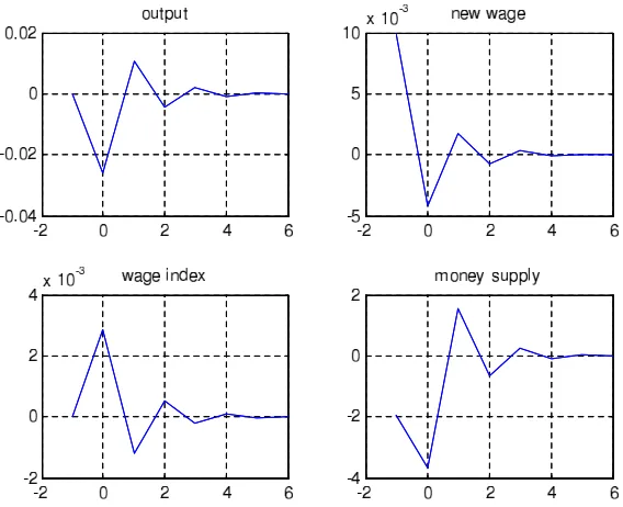
which 1₋ σ ₋γ < 0 holds.13 _{Figure 2.2 illustrates the resulting path of} 13

(40)

the economy. As in the case of constant returns to scale, we observe strong

oscillations in both nominal and real variables after the disinflation policy

is applied. The new wage falls on impact, oscillates for a few periods, and

then gradually converges to its ZISS value. Money supply and output behave

similarly. Moreover, average output from period zero onwards is substantially

lower than prior to the application of the policy. The policy therefore not

only increases macroeconomic volatility but also creates a slump in output.

In the impact period of the policy, there is a drop of more than 2 percent in

real activity.

These results are somewhat similar to the previously discussed special

case of constant returns to scale in the production function. However, the

crucial difference is that the economy converges over time after some periods

of increased volatility. The reason is related to the assumption of decreasing

returns to labor. As discussed previously, firms now face upward sloping

marginal cost curves, which relieves wages of part of the burden of responding

to desired changes in the price level or its growth rate.14 _{And the weaker is}

the response of wages in the impact period of the shock, the weaker will be the

response in the subsequent period. Hence, the magnitude of the fluctuations

in the economy decreases over time. The smaller is σ, the more rapidly this process takes place. The attenuating effect is strengthened the greater is

the elasticity of substitution between labor types ε and the greater is the elasticity of the disutility of labor ζ. 15

14

The intuition is simple: in the presence of an upward sloping marginal cost curve, the initial fall in output relieves wages from part of the burden of responding to the change in prices.

15

(41)

[image:41.612.160.437.76.309.2]

Figure 2.3: Closed Economy: Post-Disinflation Path without Oscillations

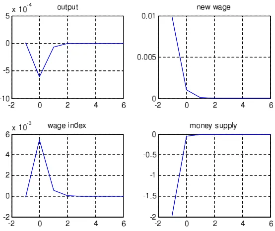
Let us now focus on the case of 1₋σ₋γ >0 in which σ is small enough and ε and ζ are large enough such that there are no oscillations in the post-disinflation state. I choose σ = 0.1 and leave all remaining parameter values the same as in the previous case. Figure 2.3 shows that there are now indeed

no oscillations in the post-disinflation path of the economy. All variables

monotonically converge to their ZISS levels. In fact, the post-disinflation

path of output reminds us of the one that is typically attained under a

conventional disinflation policy in a model with a staggering structure in

wages or prices.

To sum up, the analysis has shown that a strict inflation targeting policy

employed to reduce CPI inflation will result in a slump in output on impact

(42)

and may create oscillations of a substantial magnitude in both nominal and

real variables. The presence of oscillations in the post-disinflation path of the

economy crucially depends on the degree of returns to labor in the production

function. For a large enoughσthe disinflation policy will result in oscillatory behavior of both real and nominal variables. These oscillations die out more

slowly over time the larger is σ and are permanent in the limiting case of

σ = 1. Finally, notice that the slump in output following the disinflation policy is tiny when there are no post-disinflation oscillations in the economy

and substantial if there are.

2.3.4 Digression: Calvo Staggering Structure

In this section I briefly show that the post-disinflation oscillations in response

to our disinflation policy would not obtain in a model with a staggering

structure as proposed by Calvo (1983). This is the reason why the policy

experiment of Yun (2005) does not lead to an equivalent conclusion.

Following Yun (2005) and much of the literature, let us consider the case

of price inflation targeting in an economy in which prices are subject to a

Calvo-type staggering structure. We can write the price index in the absence

of indexation as

P1−_ε

t = (1−α)P1

−_ε

t,t +αP1

−_ε

t−1 (2.36)

where Pt is the price index and Pt,t is the price that is chosen by the

(43)

some period t= 0. Computing the ratio of Pt andPt−₁ and imposing _PPt t−1 = 1, I find that Pt,t=Pt−₁. Thus, newly set prices in the post-disinflation state

of the economy are always equal to the prevailing price level. The reason is

that firms choose prices in a forward looking manner and face the identical

problem in every period. Since prices gradually converge, there is no source

for oscillatory behavior in the economy. The increase in macroeconomic

volatility resulting from the disinflation policy applied in our model is thus

a result that does not obtain in Calvo-type staggering models.

2.4 Discussion

The present study is motivated by the idea that inflation targeting differs

from other disinflation policies in important respects. In particular, a strict

interpretation of an inflation target allows the policymaker to tolerate no

de-viations from target. But adjusting the policy instrument such that the

infla-tion target is attained and defending the new target rigorously may preserve

inflationary distortions such as wage and price differentials to an exceptional

degree. The implications of these distortions might be severe for both real

activity and volatility in the economy.

In order to formalize this idea, I have used a Dynamic General

Equilib-rium Model with wage staggering of the type suggested by Taylor (1979a) to

consider a rather extreme case of a disinflation policy: an immediate and

per-manent reduction in the rate of CPI inflation to a newly set target. I found

that the disinflation policy not only creates a slump in output on impact,

(44)

variables along their post-disinflation adjustment path. These oscillations

can be permanent when the returns to labor in the production function are

constant. In this case only, the economy does not gradually converge to a

new steady state. Moreover, I showed that the size of the initial slowdown

in real activity and the magnitude of the oscillations are positively related.

From a modeling perspective, the analysis has shown that the presence

of oscillations along the adjustment path would not occur in a model with a

Calvo (1983) type staggering structure as in Yun (2005). In the framework

of the particular model I employed, I found that the presence of oscillations

along the post-disinflation path of the economy as well as their magnitude

strongly depend on the desired size of the reduction in the inflation rate

as well as the returns to labor in the production function. In particular,

I illustrated that there are no oscillations at all along the post-disinflation

path of the economy if the returns to labor are sufficiently low. At the other

extreme, in the case of constant returns to scale, the oscillations are large

and permanent. The reason is that, in the latter case, CPI inflation targeting

becomes equivalent to a policy of wage inflation targeting.

The present study is in line with the analysis of Yun (2005) in that it

identifies the slow convergence of prices as the major source of inefficiency

resulting from an unexpected, immediate and permanent reduction in the

inflation rate. Moreover, the analysis has shown that the negative

conse-quences of strict inflation targeting identified by Svensson (2000) may be

exacerbated when the policy is used as a disinflation regime. I interpret this

as an explanation for the finding of Roger and Stone (2005) that target misses

(45)

that monetary authorities in these economies should be particularly eager to

avoid credibility losses.16 _{In sum, there are good reasons to be cautious when}

adopting inflation targeting as a disinflation regime. This may be

particu-larly true for emerging market economies which have a limited experience

with an independent monetary authority.

16

(46)

Chapter 3 Strict Inflation Targeting as a

Means of Achieving

Disinflation: Extensions

3.1 Introduction

In this chapter, I investigate how the conclusions from the previous chapter

change in an open economy setting. In addition to the returns to scale in

the production function, the degree of openness of the economy is identified

as a decisive factor in determining the presence and the magnitude of the

oscillations in the post-disinflation state of the economy. I show that the

degree of openness matters because the exchange rate acts as a stabilizer

along the post-disinflation path of the economy by effectively relieving wages

of part of the burden of reducing the inflation rate. The more open is the

(47)

Furthermore, I investigate the impact of the disinflation policy on the

economy in the full nonlinear model (as opposed to using a loglinear version

of it as in the previous and the first part of the current chapter). Although

the results are qualitatively very similar to the loglinear economy, a set of

additional conclusions emerges in the special case of a closed economy with

constant returns to scale in the production function. It turns out that the

pol-icymaker faces a surprisingly strict feasibility constraint that does not allow

for the policy to be carried out in virtually any case of empirical relevance.

The rest of the chapter is organized as follows. In Section 3.2, I extend

the model economy employed in the previous chapter to an open economy

framework. Section 3.3 identifies the degree of openness as a decisive factor in

determining the impact of the disinflation policy on macroeconomic volatility.

Section 3.4 investigates the disinflation policy in the framework of the full

nonlinear model. Section 3.5 concludes.

3.2 Opening up the Model Economy

I now assume that the economy is open in the sense that its agents trade

goods and assets with a foreign country. The economy’s basic structure is

the same as in the previous section. In opening up the economy I follow the

formulation of Fender and Rankin (2008).

I assume that there are now two output sectors, one producing tradable

goods and one producing non-tradable goods. Output in the tradables sector

YT t is exogenous and normalized to one. The production function for

(48)

specification. Markets for both types of goods are perfectly competitive.

The foreign currency price of tradables is normalized to unity. Together with

the assumption that the law of one price holds, this implies that PT t = Et,

where Et is the nominal exchange rate, i.e. the domestic price of foreign

currency. As regards financial markets, Bt is now an international bond

traded between home and foreign agents. The currency of its denomination

is immaterial since we assume that there are no initial outstanding bonds and

there is no uncertainty after the disinflation policy is applied. A no-arbitrage

condition implies interest rate parity

It=It∗

Et+1

Et

(3.1)

where I∗

t is the foreign gross interest rate. The optimization problems

of the individual agents are equivalent to the closed economy case except

that households now consume both non-tradable and tradable goods. Their

preference structure is revealed by the composite consumption index

Cjt=CN jtα C1

−α

T jt (3.2)

where 0 < α < 1 and CN jt and CT jt denote household j’s

consump-tion of nontradables and tradables respectively. Utility from consumpconsump-tion

is maximized subject to a given nominal spending constraint Sjt defined by

Sjt=PN tCN jt+PT tCT jt, such that

(49)

CT jt= (1−α)St/PT t (3.4)

where α is the degree of home bias in consumption. I denote 1₋α the degree of openness of the economy. The consumer price index (CPI) is then

a weighted average of the price of tradables and non-tradables. In particular,

Pt=

Pα N tP1

−_α

T t

αα₍₁₋_α₎1−_α (3.5)

The trade balance Tt can be expressed as Tt = 1 −CT t. In principle,

the trade balance may be different from zero, indicating a trade surplus or

deficit. Over time deficits must be balanced by surpluses and initial net

foreign assets. A modified no-Ponzi game condition therefore reads

−I−₁B−₁ = ∞ X

t=0

[I0I1...It−₁] −₁

PT tTt (3.6)

However, Fender and Rankin (2008) show that the assumptions of zero

initial net foreign assets and the exogeneity of output in the tradables sector

together imply that the trade balance is zero at any point in time. This

result significantly simplifies the analysis as it allows to abstract from any

dynamics introduced by the accumulation of net foreign assets. As in the

pre-vious chapter, we differentiate a reference zero inflation steady state (ZISS)

around which the equilibrium conditions are linearized from a constant

infla-tion steady state (CISS) in which the economy finds itself one period before

the disinflation policy is applied. The log-linear definitions and equilibrium

conditions of the open economy model can be found in Appendix A.2.1,

(50)

refer-ence steady state values.

Notice that in what follows I will distinguish between the reference zero

inflation steady state (ZISS) around which the equilibrium conditions are

linearized and a constant inflation steady state (CISS) in which the

econ-omy finds itself one period before the disinflation policy is applied. As the

economy is closed, bond holdings are zero in both states.1 _{The linearized}

equilibrium conditions are presented in Appendix A.1.1.2 _{In the following,}

lower-case symbols denote log deviations of variables from their reference

steady state values, i.e. vt =log_VV_Rt.

3.3 The Role of the Degree of Openness of

the Economy

In opening up the model economy I left its basic structure unchanged. This

implies that the initial constant inflation steady state (CISS) is the same

as in the previous section. I can thus directly proceed to derive the

post-disinflation path of the open economy. The post-disinflation policy is defined

in the exact same way as before and is applied to reduce the rate of price

inflation from its initial rate µI to the new targetµD in period t= 0. I begin

the analysis by noticing that price inflation in period t can be expressed as

pt−pt−₁ = (1−ασ)(e_t−e_t−₁) +ασ(w_t−w_t−₁) (3.7)

1

While this must necessarily be the case in a closed economy setting, I will impose it upon the open economy by assumption in the next section

2

(51)

This implies that a reduction in CPI inflation can be the result of a

re-duction in wage inflation, an exchange rate appreciation or both.3 _{It suggests}

that the post-disinflation path of wages may be subject to oscillations of a

smaller magnitude than in the closed economy model if the exchange rate

adjusts to alleviate them from part of the burden of reducing the inflation

rate. In order to investigate this issue, I proceed as in the previous chapter

and express the wage setting condition as

xt=

1 1 +β[

2γ

1 +γ(

1

1₋ασpt−

1 2

ασ

1₋ασ(xt+xt−1)) +

1₋γ

1 +γxt−1]

+ β

1 +β[

2γ

1 +γ(

1

1₋ασpt+1−

1 2

ασ

1₋ασ(xt+1+xt)) +

1₋γ

1 +γxt+1] (3.8)

Notice that setting α = 1, we are back at equation (2.32), the post-disinflation law of motion in the closed economy setting. The subsequent

steps are thus equivalent to the analysis in the previous section. I again

define φt = xt−pt. The law of motion of the open economy in the

post-disinflation state is then given by

φt+1−

1 +β β

1₋ασ+γ

1₋ασ₋γφt+

1

βφt−1 =µD(

1₋β β −

2γ

1₋ασ₋γ) (3.9)

The stability proof in Appendix A.1.2 shows that (3.9) is saddlepoint

stable as one of its eigenvalues lies within and the other outside the unit circle.

3

Essays in international monetary economics

Essays in International Monetary Economics

Christian Saborowski

Contents

List of Figures

List of Tables

Acknowledgements

Chapter 1

Introduction

Chapter 2

Strict Inflation Targeting as a

Means of Achieving

Disinflation: A Basic Analysis

2.1

Introduction

2.2

The Model Economy

2.3

Strict Inflation Targeting as a

Disinfla-tion Policy

2.3.1

The Initial Constant Inflation Steady State

2.3.2

The Special Case: Constant Returns to Scale

2.3.3

The General Case: Decreasing Returns to Scale

2.3.4

Digression: Calvo Staggering Structure

2.4

Discussion

Chapter 3

Strict Inflation Targeting as a

Means of Achieving

Disinflation: Extensions

3.1

Introduction

3.2

Opening up the Model Economy

3.3

The Role of the Degree of Openness of

the Economy