Multiresolution volumetric texture segmentation

University of Warwick institutional repository: http://go.warwick.ac.uk/wrap

A Thesis Submitted for the Degree of PhD at the University of Warwick

http://go.warwick.ac.uk/wrap/67756

This thesis is made available online and is protected by original copyright. Please scroll down to view the document itself.

Multiresolution Volumetric

Texture Segmentation

Constantino Carlos Reyes-Aldasoro

Thesis submitted to The University of Warwick

for the degree of Doctor of Philosophy

Department of Computer Science November 30, 2004

CONTENTS

Contents

Acknowledgements

Declaration

Summary

Acronyms and Notation

1 Introduction

1.1 Volumetric Texture Analysis. 1.2 The Spatial and Fourier Domains . 1.3 Sub-band Filtering . . . . 1.4 Definition of Volumetric Texture 1.5 Multiple Resolution in Texture 1.6 Classification of the Space . 1.7 Objectives of the Thesis .. 1.8 Contributions of the Thesis 1.9 Outline of the Thesis . 2 Texture Analysis

2.1 Spatial Domain Measurements 2.1.1 Single Element Mappings 2.1.2 Neighbourhood Filters. 2.1.3 Convolutional Filters . . 2.2 Wavelets... 2.3 Co-occurrence Matrices .

2.3.1 20 Co-occurrence 2.3.2 3D Co-occurrence 2.4 Frequency Filtering . . . .

2.4.1 Sub-band Filtering with Gabor Filters .

2.4.2 Sub-band Filtering with Second Orientation Pyramid 2.5 Local Binary Patterns and Texture Spectra

2.6 The Trace Transform.

2.7 Summary . . . .

CONTENTS

3 Classification

3.1 Classification . . . . 3.2 Local Energy Function . 3.3 Classifiers...

3.3.1 K-Nearest Neighbours

3.3.2 Learning Vector Quantisation (LVQ) 3.3.3 Unsupervised methods .

3.4 Summary . . . .

4 The Feature Space

4.1 Feature Selection and Extraction 4.2 The Bhattacharyya distance . . . 4.3 The Bhattacharyya Space . . . . . 4.4 Order Statistics for Feature Ranking 4.5 Summary . . . .

5 Multiresolution Classification 5.1 Climbing the Tree / ' . . 5.2 Descending the Tree \., . . . 5.3 Butterfly filters . . . .

5.4 Supervised Single Resolution vs. Unsupervised Multiresolution 5.5 Positional Contiguity Enhancing Features . . .

5.5.1 Clustering with the PCE features . . . . 5.6 Compal'ison to Markov Random Fields Models 5.7 Summary . . . .

6 Results and Discussion 6.1 2D Natural Textures. 6.2 3D Artificial Textures

6.3 3D Magnetic Resonance Textures . 6.3.1 MRI Supervised classification 6.3.2 MRI Unsupervised classification 6.3.3 Segmentation of the cartilage 6.4 Summary . . . ..

7 Conclusions

7.1 Summary . . . . 7.2 Major contributions of this work . 7.3 Major conclusions from this work. 7.4 Suggestions for further research

A Publications

B Trees and Pyramids

C Magnetic Resonance Imaging

CONTENTS iii

LIST OF FIGURES iv

List of Figures

1.1 Signals in spatial and Fourier domains . . . 5 1.2 Sub-band filtering in the Fourier domain. . . 7 1.3 Ingredients that can be identified in spatial textures 10 1.4 Volumetric texture examples . . . 11 1.5 A tree to reduce the uncertainty in the distribution; different parameters 13 1.6 A tree to reduce the uncertainty in the distribution; similar parameters 14

1.7 A classification problem . . . 15

1.8 Graphical overview of the thesis 18

2.1 Oriented pattern data . . . 20

2.2 Mapping functions of the grey level . 21

2.3 Two images (MRI and oriented) and their histograms 23 2.4 Thresholding effect on 3D sets . . . 24 2.5 Four moments for one slice of the examples: (a) Mean, (b) Standard

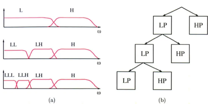
Deviation, (c) Skewness, (d) Kurtosis. . . .. 26 2.6 (a) Wavelet decomposition by successively splitting the spectrum. (b)

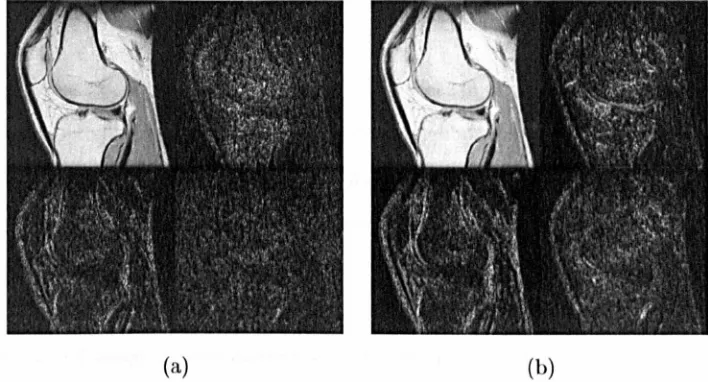
Schematic representation of the decomposition. . . 32 2.7 Wavelet packet decomposition. . . . 32 2.8 A schematic representation of a 3D Wavelet decomposition. • . . . . .. 33 2.9 Two levels of a 2D Wavelet decomposition of one slice of the human knee

LIST OF FIGURES v

2.23 Band-limited 20 Gaussian filter (a) Frequency domain p~, (b) Magnitude

of spatial domain

IPil. ...

52

2.24 A graphic example of sub-band filtering . . . .. 54 2.25 Human knee MRl and its SOP filtering . . . 55 2.26 The texture spectrum and its corresponding filtered image of (a,b)

Ori-ented data, (c,d) Human knee MR!. . . . 56 2.27 Filtered versions of the oriented data with different labellings (a,b)

Fil-tered data, (c,d) arrangements of Ei. . . . 57 2.28 The Trace transform parameters. . . . 59 2.29 Three examples of the Trace transform of the Oriented Pattern 60 2.30 A multitextured Image. . . . 61 3.1 Composite texture images arranged by Randen and Hus0y [124]. 66 3.2 Classification of elements in a set S . . . 68 3.3 The scaling of the measurements can yield different structures. . 69 3.4 Misclassification rates with different sizes of the LEF. . . . 72 3.5 Classification with different sizes of the Gaussian LEF for smoothing. 72 3.6 Four cases of spaces in 20 with two classes and different distributions 73 3.7 Visualising the measurement space and the estimates of the means . .. 74 3.8 Classification with several neighbours associated to each class. . . .. 75 3.9 Nine elements per class to be used as neighbours for classification: (a)

Randomly selected, (b) Trained as self-organising feature maps (SOM). 76 3.10 Time comparison of classification to one point or several points 79 4.1 Scatter plots of good and bad features for discrimination. 83 4.2 State space for sequential selection . . . 86 4.3 The Bhattacharyya distance. . . 88 4.4 Measurement

8

and Bhattacharyya BS[p spaces for a textured image 91 4.5 Marginals of the Bhattacharyya space . . . ~ . . . .. 92 4.6 State Space for sequential selection following the route determined from

the Bhattacharyya space. . . .. 93 4.7 Misclassification error for the sequential inclusion of features to the

clas-sifier for the 16-c1ass natural textures image (figure 3.1 (f)). 94 5.1 A pyramid to reduce the uncertainty of a filtered texture image. 99 5.2 Misclassification at every level of a Quad Tree. . . 100 5.3 Variance of the central SOP filters measurements . . . 101 5.4 Inheritance of properties to children elements . . . 101 5.5 Classification errors due to averaging of neighbouring elements. 103 5.6 2D and 3D Butterfly filters . . . . . . 104 5.7 Scalar gain a. . . . 105 5.8 A feature space view of boundary refinement process with butterfly filters 106 5.9 Classification of figure 5.1 (b): (a) Classes as levels of grey, (b) Individual

Classes. . . , . . . .. 107 5.10 Classification of a 16-class natural texture image . . . . . 108 5.11 Joint density (scatter plot) and marginal densities of the grey levels of

LIST OF FIGURES vi

5.12 (a) Classification of (82_{)6 with the new features}

_n,c

_{into 16 classes. (b)} Individual Classes . . . 111 5.13 Clustering of grey levels of figure 5.1 (a) without the new features

n,c

(b) with the new features

n,c. . . . ..

111 5.14 Clustering of grey levels of figure 5.1: (a) Marginal of figure 5.13 (a) over

C, (b) Marginal of figure 5.13 (b) over C. . . . 112 5.15 The effect of classifying noise with and without PCEs 113 5.16 Multiresolution Markov structures . . . 114 5.17 Classification of a 16-class natural texture image . . 115 6.1 Boundary classification of the images in figure 3.1 . 121 6.2 Classification as levels of grey of the images in figure 3.1 122 6.3 Correct classification of the images in figure 3.1 123

6.4 Two volumetric test data sets. . . 124

6.5 Gaussian volumetric test data. . . 125

6.6 Classification results for Gaussian data. 126

6.7 Classification of the oriented data 126

6.8 One sample slice from the knee set . . . 128

6.9 SOP Measurements for the sample slices . . 130

6.10 Bhattacharyya space B8 of a human knee MRI 131

6.11 Human knee MRI and its classification. . . 132 6.12 Volume rendering of the segmented bone of Case 1 (misclassification 8.1 %).133 6.13 A graphical representation of the features selected for the unsupervised

classification. . . .. 133 6.14 Case 2: Human knee SPGn weighted MRI. . . .. 134 6.15 (a) Sagittal slice 45 of Case 2. (b) Corresponding classification which will

be used to obtain a set of means. . . .. 134 6.16 Case 3: Human knee SPGR weighted MRI. . . .. 136 6.17 Two different angles of the segmented bone

b

(as clouds of points) from

Case 3 MRI of the human knee . . . 137

6.18 Histograms of Case 2 and Case 3 MRIs. 138

6.19 Extraction of the cartilage. . . 139

6.20 Cartilage segmentation: Case 2 . . . 139

6.21 Sagittal, coronal and axial view of the extracted cartilage 140 6.22 Rendering of segmented cartilage . . . 141 6.23 One slice of the S for the oriented texture data 143 6.24 Histograms of the measurements of S. . . 144 B.1 The structure of a Quad Tree with 4 levels. . . . 152

B.2 Parent-child structure of a Gaussian Pyramid. . 152

B.3 Gaussian Pyramid constructed from a MIU of a Human Knee. 154 B.4 Three different levels of a Laplacian Pyramid constructed from a MRI

slice of a human knee. . . 155

C.1 Nuclear Magnetic Resonance Process. 158

LIST OF FIGURES vii

LIST OF TABLES viii

List of Tables

1.1 Psycho-visual properties of Texture. . . . 8

2.1 Characteristics of the co-occurrence matrix . . . 36 2.2 Textural features of the co-occurrence matrix [55] [56]: 40 2.3 Notation used for the co-occurrence matrix and its features [55] [56] 41 2.4 Some functionals for Trace (7;), diametrical P and circus ~.. . . . . 60 3.1 Comparative misclassification results (%) of the natural textures

(fig-ure 3.1) with and without normalising the meas(fig-urement space. . . . 69 3.2 Comparative misclassification results (%) of the natural textures . . . . 70 3.3 Comparative misclassification results (%) of Sub-band filtering with Local

Energy Function (LEF) . . . 71 3.4 Comparative misclassification results (%) of the natural textures

(fig-ure 3.1) with different classification techniques. . . . . 76 3.5 Comparative time (8) results of the natural textures (figure 3.1) with

different classification techniques. . . 79 3.6 Results for unsupervised classification with LDG algorithm. . . 80

4.1 Mean, variance and Dhattacharyya distance of the human knee MRl 89 4.2 Feature Selection through the Dhattacharyya Space. . . . . . 95

5.1 Comparative miscla..qsification

(%)

with different algorithms for the im-age 3.1 (f). . . . 116

6.1 Characteristics of the images and their classification details 119 6.2 Comparative misc1assification (%) results of [104], [124], [112] and M-VTS 119 6.3 Misc1assification Results (%) for LBG and M-VTS for the two 3D test

sets. . . , . . . , . . 126 6.4 Characteristics of the MRl knee sets. . . . . 127 6.5 Misclassification results (%) for 2D and 3D single resolution and M-VTS

for Case 1 of the MRI sets. . . . 129 6.6 Classification (%) of Done (b) according to the mask for bone (b) • • •• 135 C.1 Imaging Technologies commonly used for breast cancer screening and

diagnosis . . . . C.2 Magnetic Resonance; advantages and disadvantages. C.3 Two Magnetic Resonance Protocols. . . .

ix

Acknow ledgements

This work was conducted within the Signal and Image Processing Research Group in the Department of Computer Science at the University of Warwick with the support of The University of Warwick, Consejo Naeional de Ciencia y Teenologia CONACYT and In-stituto Tecnol6gico Aut6nomo de Mexico ITAM, in particular Dr. Federico Kuhlmann. I am grateful to all of them.

I am very grateful to my supervisor Dr. Abhir Dhalerao for the support and guidance through the years at Warwick; he was always ready to help anyone who asked his advice, he always had time for a chat and always challenged our ideas to help us produce better results. Thank you.

I would like to thank Dr. Trygve Randen from Schlumberger Stavanger Research in Norway for providing the natural texture images and Dr. Simon Warfield from Brigham and Women's Hospital in Doston, USA who provided some of the MRI data sets that were used in this thesis and also kindly revised some of the results.

I would also like to thank Dr. Nasir Rajpoot, Prof. Roland Wilson and Dr. Chang-Tsun Li for the helpful comments I received from them.

I shared several labs with different people during these years: Xiaoran Mo, Vincent Ng, Denis Fan and Li Wang. I enjoyed sharing the process of a PhD with you all.

Declaration

I declare that, except where acknowledged, the material contained in this thesis is my own work and that it has neither been previously published nor submitted elsewhere for the purpose of obtaining an academic degree.

Summary

M ultiresolution Volumetric Texture Segmentation

Constantino Carlos Reyes-Aldasoro

Thesis submitted to The University of Warwick for the degree of Doctor of Philosophy

30 November, 2004

xi

This thesis investigates the segmentation of data in 20 and 30 by texture analysis using Fourier domain filtering. The field of texture analysis is a well-trodden one in 20, but many applications, such as Medical Imaging, Stratigraphy or Crystallography, would benefit from 3D analysis instead of the traditional, slice-by-slice approach. With the intention of contributing to texture analysis and segmentation in 30, a multiresolution volumetric texture segmentation (M-VTS) algorithm is presented.

The method extracts textural measurements from the Fourier domain of the data via sub-band filtering using a Second Orientation Pyramid. A novel Bhattacharyya space, based on the Dhattacharyya distance is proposed for selecting of the most discriminant measurements and produces a compact feature space. Each dimension of the feature space is used to form a Quad Tree. At the highest level of the tree, new positional features are added to improve the contiguity of the classification. The cla.~sified space is then projected to lower levels of the tree where a boundary refinement procedure is performed with a 3D equivalent of butterfly filters.

The performance of M-VTS is tested in 20 by cla.<;sifying a sct of standard texture images. The figures contain different textures that are visually stationary. M-VTS yields lower misclassification rates than reported elsewhere ([104, 111, 124]).

Acronyms and Notation

M-VTS sOP

LBG

eNS WM

GM

MRI

SPGR

Tr Te

peA

LEF

TU

NTu

LBP

LVQ SaM kNN

peE

MRF MMRF ROI/VOI BS BF

QT

TLE

FeD

MFT

Multiresolution Volumetric Texture Segmentation Second Order Pyramid

Linde Buzo Gray Vector Quantising Algorithm Central Nervous System

Brain White Matter Brain Grey Matter

Magnetic Resonance Imaging Gradient Echo Pulse Sequences Repetition Time

Echo Time

Principal Components Analysis Local Energy Function

Texture Unit

Texture Unit Number Local Binary Pat tern

Learning Vector Quantisation Self-Organising Feature Maps k Nearest Neighbours

Positional Contiguity Enhancing (Features) Markov Random Fields

Multiresolution Markov Random Fields Region/Volume of Interest

Bhattacharyya Space Butterfly Filter Quad Tree

Temporal Lobe Epilepsy Focal Cortical Dysplasia

Multiresolution Fourier Transform

VV I

f(r) r,c,d

Nr,Nc,Nd

Lr = {1,2, ...

,r, ...

,Nr} Lc = {1,2, ...

,c, ...

,N_c} Ld = {1,2, ... ,d, ... ,Nd} Lr x Lc X Ld

X = (r,c,d) E Lr x Lc x Ld VV(x) = g, 9 E G

Ng

G= {1,2, ... ,g, ... ,Ng } h(g)

JV C (Lr x Lc x Ld)

VV(x) = T[VV(JV)]

T

VVw

=

9"[VV] p,K,O

:Fn Fi / F~

VVV

=

8VV f

+

8VV

e

+

8VV

d

(JT iJC

aa

f,e,d

Volumetric data Image data

A ID function of r

Co-ordinates of the spatial domain: rows, columns, slices

Number of rows, columns and slices Rows domain

Columns domain Slices domain

Dimensions of the volumetric data An element of the volumetric data Grey levelj Intensity associated with el-ement x

N umber of grey levels Quantised grey level domain Histogram of the data

A neighbourhood of an element of the space

Dimensions of the neighbourhood An operator on the volumetric data around the neighbourhood JV

Operator associated to measurement i Fourier transform of VV

Co-ordinates for the Fourier domain Fourier coefficients

A filter associated to measurement i in the spatial/Fourier domains

A Gabor filter in the spatial/Fourier domain

Volumetric data VV filtered by filter F~ (Fourier domain)

Volumetric data VV filtered by filter Fi (Spatial domain)

Gradient operator over the volumetric data

Unitary vectors in the direction of the axes

S

Si

=

VV

i Si(X) = g,

S(X) = {Sl(X), ... , SNi(X)}

S(x) E

_,

G x Gx, ... ,G

_,

...

~a

§i = Si

*

~a Si _w

Ni

Ni

Li = {I, 2, ... , i, ... , Ni} Lr x Lc X Ld X Li Lj={ ... ,j, ... ,} SpeS

Lf eLi

Lr x Lc X Ld xLI SI ESp, SI E S Jl.

8 ku (-, .)

II .

112

Z

lR C

Space of the measurements over the data Measurement i over the data

The value of element x at measurement i

A vector (pattern) of the values of element x at every measurement

Domain of the measurement vector

A Gaussian function

A smoothed version of Si

Fourier transform of measurement i

N umber of measurements over the data Measurement domain

Dimensions of the measurement space

A permutation of the measurement domain Feature space extracted from the measure-ment space

Number of features selected from the mea-surement space

Feature domain

Dimensions of the feature space

A feature Mean Standard deviation Skewness Kurtosis Inner product Norm

The set of integers numbers The set of real numbers The set of complex numbers

mw a(t)

JVu,

Rk cS

Lk = {1,2, ... ,Nk } (kl, k2)j k1 , k2 E Lk

Np

Lp = {(I, 2), ... , (k1 , k2),

... ,(Nk - I,Nk)}

D

D2

DB

DB(k1 , k2 ) BSIP BS[,BSp

Labelling function

Approximation of labelling function (Classifier)

Description of a class through a single pointj the points ak define hyperplanes perpendicu-lar to the chords that connect them

Description of a class with n points per class An estimate of the mean / prototype values for a certain class k

N umber of classes

Number of Nearest Neighbours

A reference vector (neuron) associated with class i

A winner neuron (closest to input signal x) in a competitive process

A monotonically decreasing scalar gain factor A neighbourhood around the winner neuron Regions corresponding to a partition of S Classes domain

A pair of classes Misclassification error N umber of pairs of classes Domain of pairs of classes

A distance measure

Euclidean distance measure Chess-board distance

Bhattacharyya distance measure Bhattacharyya space

Marginal distributions of the Bhattacharyya space

Order statistics of the marginal distributions of the BS

v =

{O,o, ... ,O}

v' = {I, 1, ... ,I} (QT)C (gp)C (gp)C,n (G)C 8,¢ <{)1,<{)2,···

n,c,v

1/;( r) 1/;k,l(r) w(k,l) Ck,l

Tr,

P, cI>

ls,rw

N

_w

Slw(x)/ S~w(x)

Initial state for feature selection Final state for feature selection Quad Tree (QT) at level

.c

Gaussian Pyramid (gp) at level

.c

n Expansions of (gp)C

Grey level/ Intensity associated with the data of a Quad Tree at level C

Un-normalised co-occurrence matrix, as a function of two grey levels, distance and ori-entation

Orientation measures

Textural features of the co-occurrence matrix Row, Column and Slice co-ordinates, (PCE features)

A mother Wavelet

Scaled and dilated Wavelet Wavelet transform

Coefficients of Wavelet transform

Trace, diametrical and circus functionals of the Trace transform

The set that describes the elements of each wing (left/right) of the butterfly filters Number of elements in lw/rw

Weighted average of the grey levels of lw/rw Weight function for the elements of the filters Number of elements that share class with the pivot element x.

The weighted combination of the element

x

and

Slw/S:w

1

Chapter 1

Introduction

1.1

Volumetric Texture Analysis

The study of Volumetric Texture is a very challenging subject. To start with, there is not a single accepted definition of texture in two dimensions (2D). Then, the extra third dimension that is included in texture in three dimensions (3D) increases considerably the computational complexity. In some cases, the extension of texture analysis to three dimensions can be easily achieved, but in others, for example those using orientation or phase, careful consideration is needed.

Volumetric texture has received much less attention than its spatial 2D counterpart which has seen the publication of numerous and differing approaches for texture analysis and feature extraction (for example [8, 15, 29, 55, 56, 144, 146]), and classification and segmentation ([14, 71, 75, 79, 147, 156]).

1.1. VOLUMETRIC TEXTURE ANALYSIS 2

the volumetric texture of the patterns of seismic waves within sedimentary rock bodies can be used to locate potential hydrocarbon reservoirs. In Medical Imaging, the data provided by the scanners of several acquisition techniques such as Magnetic Resonance Imaging (MRI) [88, 128], Ultrasound [166] or Computed Tomography (CT) [65, 136] deliver grey level data in three dimensions. Different textures in these data sets can allow the discrimination of anatomical structures. The importance of Texture in Mill has been the focus of researchers, such as Lerski [94] and Schad [134], and a COST European group was established for this purpose [28].

Texture analysis has been used with mixed success in medical imaging: for detection of micro-calcification and lesions in breast imaging [72, 137, 142], for knee segmenta-tion [78,100], for the delineasegmenta-tion of cerebellar volumes [131]' for quantifying contralateral differences in epilepsy subjects [164, 165], to diagnose Alzheimer's disease [133] and brain atrophy [136], and to characterise spinal cord pathology in Multiple Sclerosis [106]. Most of this reported work, however, has employed solely 20 measures, usually co-occurrence matrices that are limited by computational cost. Furthermore, feature selection is often performed in an empirical way with little regard to training data, which are usually available.

1.2. THE SPATIAL AND FOURIER DOMAINS 3

1.2 The Spatial and Fourier Domains

The Fourier transform [16] is a well-known mathematical operation that translates a sig-nal from the spatial or time domain, into the Fourier or frequency domain. The Fourier domain will be widely used through this thesis since some of the signals that appear as texture have strong energy concentration at different frequencies and orientations. Con-sequently, different textures can be discriminated by the amount of energy that the signal displays in different frequency bands. This will be explained in detail in section 2.4.2. For example, figure 1.1 (a) presents a ID signal in the spatial domain and its transforma-tion into the Fourier domain. It can be observed that the signal appears fairly repetitive in the spatial domain, which translates into three main spikes in the Fourier domain. The basis of the Fourier transform is the analysis of exponential Fourier series, that is, the representation of a signal by the sum of the exponential signals that are orthogo-nal to each other. The exponential function e jr forms a family of orthogonal functions within a certain interval [ro, ro +

RJ

with the functions ejn21rrpo, n = 0, ±1, ±2, ... where

e is the complex Euler identity: ejn21rrpo = cos(n27rrpo)

+

jsin(n21fTpo), and Po will determine the frequency of the sinusoidals. Any signal can be expressed by a series of these functions:

:F_le-j21rrpo

+

:F_2e-j41rrPo

+

:F_3e-j61rrpo

+ ...

00

f(r) =

L

:Fnejn21rrpo n:-oo

(1.1)

where ro

< r

< ro +

Rand R =

!:.

The constants :Fn , called the Fourier coefficients of f are defined by the inner product ((-,.)) between the original signal and the exponential:

1.2. THE SPATIAL AND FOURIER DOMAINS 4

where

0*

represents the complex conjugate of a signal. Two important observations follow. First, the orthogonality of the functions Tnejn27rTPO mean that their inner product is zero:

(1.3)

The inner product of a signal with itself is called the norm:

(1.4)

and it can be used as a measure of the energy of the signal.

Second, it is important to notice that the previous analysis is limited to a certain interval in time or space. To consider the range (-00, +00) the period has to be evaluated in the limit R -t 00. By taking the limit (and after some manipulation) the Fourier transform pair is reached [16]:

f(r) =

i:

fw(p)ej27rTPdp

fw(p) -

i:

f(r)e-j27rrPdr

which is sometimes represented by:

fw

(1.5)

(1.6)

1.2. THE SPATIAL AND FOURIER DOMAINS 5

:s 0 u.

Spatial domain Fourier domain

[image:23.575.120.524.109.636.2]

1.3. SUB-BAND FILTERING 6

(1.7)

where (r, c, d) are the co-ordinates in the spatial domain and (p,~, d) are the co-ordinates in the Fourier domain.

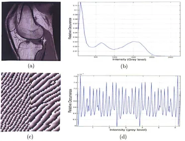
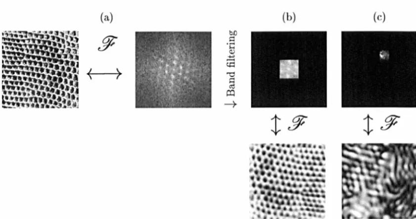
Figure 1.1 (b) shows one image with a textured pattern and its corresponding 2D Fourier transform. It can be seen that some of the ingredients or characteristics of the image are noticeable in its Fourier counterparts.

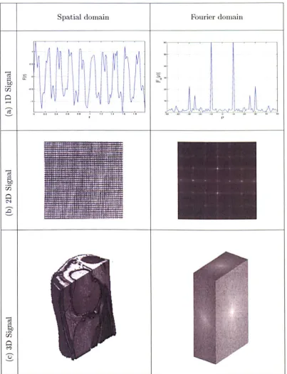
Figure 1.1 (c) presents a case of a 3D signal in the spatial and Fourier domains. The spatial data correspond to the Magnetic Resonance Imaging (MRI) of a human knee that has been sliced in the sagittal and axial planes. The Fourier domain is also sliced in the 3 axes. A description of the Magnetic Resonance Imaging technology is presented in appendix C, while a brief description of the human knee is presented in appendix D. Analysing volumetric data in this way is harder than 2D images (and often the analysis is performed slice-by-slice). However, the 3D Fourier transform allows us to work with the whole volumetric set and any operation like filtering, thresholding or convolution can be performed in 3D.

Figure 1.3 shows further examples of images with different textures. Periodicityap-pears as bright spots (equivalent to the spikes in 1D), orientation apPeriodicityap-pears perpendicular in opposite domains and the randomness appears as a signal that increases its intensity towards the centre.

1.3 Sub-band Filtering

1.4. DEFINITION OF VOLUMETRIC TEXTURE 7

(a) (b) (c)

bD

§

.9

I-< Q.) ...., ~

<

>

"0

>=I <1:l CO

4-tff

tff

Figure 1.2: Sub-band filtering in the Fourier domain: (a) An image (reptile skin) in the spatial and Fourier domains, (b) A low pass filtered version of the image, (c) A band pass version of the image.

version of the image, while a band pass filter captures other details of th texture. The principle of sub-band filtering can equally be applied to volumetric data (sec-tion 2.4.2).

1.4 Definition of Volumetric

Texture

A single definition of texture does not exist, but most of the numerous d finitions that are present in the literature, have some common elements that emerge from the etymology of the word. Texture comes from the Latin textura, the past participle of the verb texere, to weave [108]. From here, it is expected that a texture will exhibit a certain structure created by common elements, repeated in a certain regular way, as in the threads that form a fabric. Hawkins [58] identifies three ingredients of texture:

• some local 'order' is repeated over a region which is large in comparison to the order's size,

• the order consists on the non-random arrangement of elementary parts, and, • the parts are roughly uniform entities having approximat ly the same dimensions

[image:25.562.104.525.69.290.2]

1.4. DEFINITION OF VOLUMETRIC TEXTURE 8

Table 1.1: Psycho-visual properties of Texture.

Author Properties

Ravishankar [127] Granular, marble-like, lace-like, random, random nongran-ular and somewhat repetitive, directional locally oriented, repetitive.

Tamura [144] Coarseness, contrast, directionality, linelikeness, regularity, roughness.

While these ingredients can describe some textures, as those of figure 1.3 (a), there are some other cases that are not so uniform or deterministically arranged. For instance, the pebbles of figure 1.3 (b) appear to be in a random placement. The term visual texture is some times used in an attempt to distinguish it from the tactile concept of texture. From this visual context, image texture is defined by Tuceryan and Jain [146] as:

• A function of the spatial variation in pixel intensities.

Gonzalez [50] relates certain properties of texture with the approaches to texture anal-ysis:

• Statistical: smooth, coarse, grainy, ...

• Structural: arrangement of feature primitives (sometimes called textons) ac-cording to certain rules,

• Spectral: global periodicity based on the Fourier spectrum.

Some of these properties are visually meaningful and are helpful to describe textures. In fact, studies have analysed texture from a psycho-visual slant [127, 144] and have identified the properties presented in table 1.1.

It is important to notice that these properties are different from the features or measurements (although some other works refer to the properties as features of the data) that can be extracted from the textured regions.

Two more ingredients of texture should be mentioned:

1.4. DEFINITION OF VOLUMETRIC TEXTURE 9

• The texture of an element (pixel or voxel) is implicitly related to its neighbours. It is not possible to describe the texture of a single element, as it will always depend on the neighbours to create the texture. This can be exploited through: Fourier methods, which extract frequency components according to the relation of elements; a Markovian approach in which the attention is restricted to a small neighbourhood; or a co-occurrence matrix where occurrence of the grey levels of neighbouring elements is recorded.

All the properties and ingredients that were previously mentioned about texture, or more specifically, visual, or 2D texture, can be applied to volumetric texture.

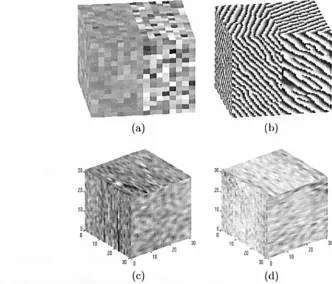
In this thesis, Volumetric Texture is considered as the texture that can be found in volumetric data (this is sometimes called solid texture [12]). Figure 1.4 shows four examples of volumetric data with some textured regions. Volumetric Texture is different from 3D Texture, Volumetric Texturing or Texture Correlation.

3D Texture [20, 31, 32, 95, 99] refers to the observed 2D texture of a 3D object that is being viewed from a particular angle and whose lighting conditions can alter the shadings that create the visual texture. This analysis is particularly important when the direction of view or lighting can vary from the training process to the classification of the images. Our volumetric study is considered as volume-based (or image-based for 2D); that is, we consider no change in the observation conditions. In Computer Graphics the rendering of repetitive geometries and reflectance into voxels is called Volumetric Texturing [110]. A different application of texture in Magnetic Resonance is the one described by the term Texture Correlation proposed by Bay

[3]

and now widely used [4, 49, 107, 119] which refers to a method that measures the strain on trabecular bone under loading conditions by comparing loaded and unloaded digital images of the same specimen.

1.4. DEFINITION OF VOLUMETRIC TEXTURE 10

(a) Non-random arrangement of elementary parts, parts are roughly uniform

§

<

)

Bricks Reptile skin in Fourier domain (b) Roughly regular parts, random arrangement

§

<

>

Sunflowers Pebbles Pebbles in Fourier domain (c) Regular parts are not identifiable, nor there is a non-random arrangement

§

<

>

Bone in a T2 MRl Wool Wool in Fourier domain

(d) Dominant orientation present, regular parts mayor may not be identifiable

§

<

>

Straw Wood Wood in Fourier domain

1.5. MULTIPLE RESOLUTION IN TEXTURE 11

(a) (b)

[image:29.558.109.442.93.377.2]

(c) (d)

Figure 1.4: Volumetric texture examples: (a) A cube divided into two regions with Gaussian noise. (b) A cube divided into two regions with oriented patterns of different frequencies and orientations. (c) A sample of muscle from MRI. (d) A sample of bone from MRI.

represented then as a function that assigns a grey tone to each triplet of co-ordinates:

(1.8)

An image then is a special case of volumetric data when Ld = {I}, that is [56]:

(1.9)

1.5 Multiple Resolution in Texture

Multiresolution methods have been widely used in image analysis problems for some

1.5. MULTIPLE RESOLUTION IN TEXTURE 12

at different scales or resolutions. Images at lower spatial resolutions are created by a recursive process of filtering and sub-sampling. The use of multiresolution techniques has been motivated by different reasons: reducing the computational complexity of the task; enabling the application of filters with increasing larger support; optimisation problems when the solution at a coarse scale can be used to initialise the solution at the next finer resolution. The reduction of image size results in a decreased complexity, opening up solutions to otherwise difficult problems. Filtering at various scales or channels can extract different measurements or features of an image, as done with Gabor or Lognormal filters [71, 81] of various sizes and orientations or the Second Orientation Pyramid tessellation [162] (section 2.4.2).

Another implication of multiresolution techniques is a trade-off between spatial res-olution or positional accuracy, and measurement uncertainty or the measurement class membership. Multiresolution pyramids [17] or trees [132, 140, 162] can be constructed by a weighted average of neighbouring elements, from lower, fine levels up to a coarse higher level where each node is considered as the parent of several child nodes. At the higher levels these trees have, on one hand, reduced uncertainty in the measurement values (grey level for instance) but inherently lower spatial resolution. Appendix D describes the construction of pyramids and trees that will be used through this thesis.

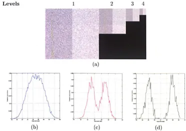
Figure 1.5 (a) shows an example of a tree of an image with two noisy regions with normal distributions that have an overlapping grey scale. At the image level, the two regions are not distinguishable in the histogram (b), but at lower spatial resolutions of a tree, the smoothing makes the classes separate from each other, as the histograms in (c,d) show. (The use of the histograms at different resolutions is sometimes called multiresolution histograms [53], a term that could be confusing since it is the images and not the histograms themselves which are in a multiresolution space.)

a-1.5. MULTIPLE RESOLUTION IN TEXTURE 13

tions such as the Multiresolution Fourier Transform (MFT), which is an over-complete, Fourier Wavelet basis [157J. In this work, we have adapted the feature estimation ideas from [162J into a new classification framework based on the work of Schroeter and Bi-gun [135J.

Levels 1 2 3 4

(a)

[image:31.576.124.496.178.441.2]

(b) (c) (d)

Figure 1.5: A tree to reduce the uncertainty in the distribution, the coarsest image contains two regions with Gaussian noise (/-Ll = 25, (71

=

5, /-L2

=

29, (72

=

5). (a) Quad Tree of 4 levels placed side by side. (b) Histogram at lowest level (level 1). (c) Histogram at level 2. (d) Histogram at level 3.

1.6. CLASSIFICATION OF THE SPACE 14

Levels 1 2 3 4

(a)

[image:32.577.124.497.105.370.2]

(b) (c) (d)

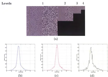
Figure 1.6: A tree to reduce the uncertainty in the distribution. When the distributions have similar mean values, the regions tend to merge into one (/LI

=

25, al

=

2, /L2

=

25.5, a2

=

5). (a) Quad Tree of 4 levels placed side by side. (b) Histogram at lowest level (level 1). (c) Histogram at level 2. (d) Histogram at level 3.

1.6

Classification of the Spac

e

The classification or labelling problem is that of assigning every clement of the data,

or the measurements extracted from the data, into one of several possible classes [54].

For medical data the classes can represent a unique anatomical structure such as a

bone, cartilage or muscle. The classifying process corresponds to a partitioning of the

space of the measurements into regions. For example, figure 1.7 presents two different

populations in a two-measurement space and the possible partitioning into two classes

with different classification schemes. The classifiers used were: thresholding that result

in a straight boundary; and LVQl, which adapts better to the original distribution.

The choice of a classification algorithm can therefore be important. When the original

1. 7. OBJECTIVES OF THE THESIS ₁₅

lealure 1 feature 1

(a) (b) (c)

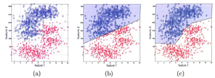
Figure 1.7: A classification problem. Two different populations are distributed over a two measurement space, (a) represents the ground truth. The populations are classified with two different strategies, first with thresholding which results in a straight boundary (b), and

with LVQl a more sophisticated classifier which results in a piecewise linear boundary (c). The colours in (b,c) represent the classes into which the elements have been assigned; (c) is closer to the ground truth.

be measured, but this is not generally the case, sometimes only estimates of the accuracy can be achieved.

There is a vast amount of literature concerned with these problems [6, 11, 36, 54J. In chapter 3 we will analyse some of the techniques that may be of use for texture classification. Two important aspects related to the classification process are: the effect of the Local Energy F\mction (LEF) and the context or positional information of the elements and not only their measurement values. This will be treated in sections 3.2 and 5.5.1 respectively.

1.

7

Objectives of the Thesis

This thesis intends to contribute to the relatively new problem of volumetric texture analysis and classification by proposing a multiresolution volumetric texture seg men-tation (M-VTS) methodology. The main goal is to provide a method that receives volumetric data (we have concentrated on MRI) and returns a series of classes with homogeneous characteristics, like anatomical structures, based on textural properties. To achieve this objective, several problems must be solved.

[image:33.578.129.501.81.217.2]

1.8. CONTRIBUTIONS OF THE THESIS 16

effective measurement space needs to be generated.

2. The number of measurements that can be extracted from the data can be con-siderable, and when working in three dimensions, it will be even greater. The reduction of dimensions of the measurement space will not only reduce the com-putational complexity but may also achieve better results through selection of the best features.

3. The measurement space needs to be classified. We require a suitable classifier that discriminates classes properly and in a reasonable time. In the MRI data, classes

will be ascribed to anatomical features.

4. The measurements extracted and the classification algorithm need to be compared against other existing techniques. The benchmark comparison is essential for all the steps of the classification process.

5. Multiresolution techniques have been proposed in other applications and it is pos-sible that texture segmentation will benefit from multiresolution algorithms. This proposition will be investigated.

1.8 Contributions of the Thesis

The original contributions of this thesis are:

1. A survey of the volumetric texture extraction methods is presented; some advan-tages and disadvanadvan-tages of the techniques are highlighted.

2. We propose an extension of the Second Order Pyramid (SOP) (based on Spann and Wilson [162]), a 2D Method, into 3D.

1.9. OUTLINE OF THE THESIS 17

4. Based on the Bhattacharyya distance, a novel Bhattacharyya Space [128] is pro-posed as a methodology to select the most discriminant features of the measure-ment space.

5. A multiresolution classification algorithm (based on [135, 162]) is extended from 2D to 3D. Some extensions of the algorithm from 2D to 3D are required; in particular the use of boundary smoothing filters. The use of a Markov Random Field (MRF) approach is compared with pyramidal butterfly filters, the latter providing superior results.

6. Context is included in the classifier to improve the results. A contiguity enhanc-ing strategy is proposed through the use of new features (Positional Contiguity Enhancing features) that are added to the feature space.

7. A series of 2D and 3D data sets are classified and compared with other method-ologies and the proposed algorithm is shown to give excellent results. Three MRIs of human knees are classified. For validation and reproducibility, the data scts generated and the code is made available on the web page:

http://www.dcs.warwick.ac. ukl -creyes

I

m-vts.

8. As an application of the methodology, it is shown how a segmentation of an anatomical structure through the proposed algorithm can be used for the extrac-tion of other structures like the cartilage.

1.9

Outline of the Thesis

1.9. OUTLINE OF THE THESIS 18

is proposed as a hierarchical methodology for the refinement of the boundaries. Also, a

new set of positional features that added to a feature space can yield better contiguity

is also proposed. Chapter 6 compares the results of the proposed methodology with

others present in the literature for 2D data. Also, volumetric data sets are presented

and classified with a special emphasis given to human knee MRls. The MRI knees are

first classified into anatomical regions and the results are used to segment the cartilage.

Finally, chapter 7 presents conclusions and proposals for further work.

c

Classified Data

19

Chapter

2

Texture Analysis: the

Measurement Space

In this chapter, a review of texture measurement extraction methods will be presented. A special emphasis will be placed on the use of these techniques in 3D. Some of the techniques have been widely used in 2D but not in 3D, and some others have already been extended. We will analyse and compare them in order to select the most adequate measurement for the data used in this thesis. We conclude that sub-band filtering with SOP in the Fourier domain is the most appropriate measurement for its simplicity and power. For visualisation purposes, two data sets will be presented: an artificial set with two oriented patterns (figure 2.1) and one volumetric set of a human knee Mill set

(figure

1.1

(c».

These sets along with several other 2D and 3D will be classified and the performance compared with different techniques in chapter 6.

2.1. SPATIAL DOMAIN MEASUREMENTS 20

§

<

>

(a) (b)

Figure 2.1: Artificial data set with two oriented patterns of [64 x 32 x 64] elements each,

with different frequency and orientation: (a) Data in the spatial domain, (b) in the Fourier domain.

discrimination of a certain class. Therefore the selection of a proper set of

measure-ments is a difficult task. In this chapter we will concentrate on the generation of the

measurements and in chapter 4, feature selection and extraction will be investigated. In

terminology of Hand [54], we will call the first set of all dimensions the measurement

space and the reduced set the feature space.

2.1

Spatial Domain Measurements

The spatial domain methods operate directly with the values of the pixels or voxels of

the data:

VV(x) = T[VV(JV)], JV

c

(Lr x Lc x Ld), x E (L{ x L{ x Lf ) (2.1)

where T is an operator defined over a neighbourhood JV (relative to the element x that

belongs to th region (L:{ x L{ x L1 )). The result of any particular operator Ti will

become one dimension of the multivariate measurement space S:

(2.2)

and the measurement space will contain as many dimensions i as the operations p

[image:38.546.142.454.81.196.2]

2.1. SPATIAL DOMAIN MEASUREMENTS 21

g

= T [g]

g=

T [g 1

g g

(a) (b)

Figure 2.2: Mapping functions of the grey level: (a) Grey levels remain unchanged. (b) Thresholding between values gl and gh.

2.1.1 Single Element Mappings

The simplest case arises when the neighbourhood JV is restricted to a single element x. T then becomes a mapping T : G -+ G on the grey level of the clement:

9

= T[g] and is sometimes called a mapping function [50]. Figure 2.2 shows two cases of these mappings; the first involves no change of the grey level, while the second case thresholds the grey levels between certain arbitrary low and high values g/, gil.

This technique is simple and popular and is known as grey level thresholding, which can be based either on global (all the image or volume) or local information. In each scheme, single or multiple thresholds for the grey levels can be assigned. The philos-ophy is that pixels with a grey level below a threshold belong to one region and the remaining pixels to another region. In any case the idea is to partition into regions,

object/background, or objecta/objectb/ ... background. Thresholding methods rely on the assumption that the objects to segment are distinct in their grey levels and use the histogram information, thus ignoring spatial arrangement of pixels. Although in many cases good results can be obtained, in MRl, the intensities of certain structures are often not uniform, sometimes due to inhomogeneities of the magnets, and therefore simple thresholding can divide a single structure into different regions. Another matter to consider is the noise intrinsic to the images that can lead to a misclassification. In many cases the optimal selection of the threshold is not a trivial matter.

2.1. SPATIAL DOMAIN MEASUREMENTS 22

certain grey levels. The histogram is defined as:

()

# {x E (L

r x Lc x Ld) : VV(x} = g} 9 E G

h 9

=

_#

{

_{Lr x Lc X Ld}

}

,

(2.3)

where

#

denotes the number of elements in the set. This approach involves only the first-order measurements of a pixel [27] since the surrounding pixels (or voxels) are not considered to obtain higher order measurements. Figure 2.3 presents the two data sets and their corresponding histograms. The histogram of the human knee (b) is quite dense and although two local minima or valleys can be identified around the values of 300 and 900, using these thresholds may not be enough for segmenting the anatomical structures of the image. It can be observed that the lower grey levels, those below the threshold of 300 correspond mainly to background, which is highly noisy. The pixels with intensities between 301 and 900 roughly correspond to the region of muscle, but include parts of the skin, and the borders of other structures like bones and tissue. Many of the pixels in this grey level region correspond to transitions from one region to another. (The muscles of the thigh; Semimembranosus and Biceps Femoris in the hamstring region, do not appear as uniform as those in the calf; the Gastrocnemius, and Soleus.) The third class of pixels with intensities between 901-2787 roughly correspond to bones - femur, tibia and patella - and some tissue - Infrapatellar Fat Pad, and Suprapatellar Dursa. These tissues consist of fat and serous material, which have similar grey levels as the bones. The most important problem is that bone and tissue share the same range of grey levels in this MID and using just thresholding it would not be possible to distinguish successfully between them.

2.1. SPATIAL DOMAIN MEASUREMENTS 23

1000 1000

Intensity (Grey level)

(a) (b)

. 10·

~ ,. t:: '

.§

••

~v

J

..,

~ ee

C2

_II

.

Intensltyil(grey leV~l)

(c) (d)

Figure 2.3: Two images (one slice of the data sets) and their histograms: (a, b) Human Knee MRI, and (c, d) Oriented textures.

are not background, the inhomogeneity of the magnetic field with which the image was

acquired causes the effect of background. This problem will not be addressed in this

work.

The histogram of the oriented textures (figure 2.3 (d)) is not as dense and smooth

as the one corresponding to the human knee and it spreads through the whole grey level

region without showing any valleys or hills that could point out that a thresholding

[image:41.563.125.497.82.366.2]

could help in discrimination the textures involved.

Figure 2.4 shows the result of thresholding over the data sets previously presented.

The human knee was thresholded at the 9

=

1500 and the oriented data at 9

=

5.9.

For the knee some structure of the leg is visible (like the Tibia and Fibula in the lower

part) but this thresholding is far from useful. For the oriented data both regions contain

2.1. SPATIAL DOMAIN MEASUREMENTS 24

(b) ( c)

Figure 2.4: Thresholding effect on 3D sets: (a) Oriented textures thresholded at 9

=

5.9. (b) Human knee thresholded at 9 = 1500.

2.1.2 Neighbourhood Filters

When T comprises a neighbourhood bigger than a single element, several important

measurements arise. When a convolution with kernels is performed, this can be con -sidered as a filtering operation, which is described below. If the relative position is not

taken into account, the most common measurements that can be extracted are stati

s-tical moments. These moments can describe the distributions f the sample, that is

the elements of the neighbourhood, and in some cases these can help to distinguish different textures. Yet, since they do not take into account the particular position of any pixel, two very different textures could have the same distribution and therefore the same moments. Even with this limitation, some researchers use these measurements as

descriptors for texture. Acha [1] performed burn diagnosis to distinguish healthy skin from burn wounds. Their textural measurements were a set of parameters; mean, stan

-dard deviation, and skewness, of the colour components of their images. Their feature

selection invariably selected the mean values of lightness, hue, and chroma, so perhaps

the discrimination power resides in the amplitude levels more than the texture of the

images. Kapur [78] studied 3D medical data in a model-based analysis where a spatial

relationship, measuring distance and orientation, between bone and cartilage is modelled

2.1. SPATIAL DOMAIN MEASUREMENTS 25

Lorigo [100] performed segmentation of the bone in MRI using active contours. Both used local variance as a measure of texture.

For a neighbourhood related to the element x = (r, c, d) a neighbourhood can be seen as a subset JY of the data with the domains

L{ x L{ x Lf (of size

N(, N;r, Nf) related to the data in the following relations:

L{CLr L{={r,r+l, ... ,r+N;t'}, l~r~Nr-N;t', (2.4)

L{CLc L{={c,c+l, ... ,c+Nt'}, l~c~Nc-Nt', (2.5)

Lf C Ld L{

=

{d,d+ 1, ... ,d+ Nf}, 1 ~ d ~ Nd - Nf, (2.6)

(r,c,d) E (L{ x L{ x Lf) (2.7)

The first four moments of the distribution; mean J.1" standard deviation u, skewness 8 and kurtosis ku, are obtained by:

1

J.1,vv = N.A' N.A' N.A'

L

VD(r, c, d) (2.8) r e d L.K xL.K xL.K _{r e d}

(2.9)

(2.10)

(2.11)

Figure 2.5 shows the results of calculating the four moments over a neighbourhood of size 16 x 16 in a sliding way (overlapping) for the two previous data sets. It is important to mention that for higher moments the accuracy of the estimation will depend on the number of points. With only 256 points, the estimation is not very accurate.

2.1. SPATIAL DOMAIN MEASUREMENTS 26

(a) (b) (c) (d)

Figure 2.5: Four moments for one slice of the examples: (a) Mean. (b) Standard Deviation. (c) Skewness. (d) Kurtosis.

more than 92% of the total elements.

While for the knee data, some of the results can be of interest, for the oriented

textures the moments resemble a blurred version of the original image. From here we

can observe that if these moments are of interest it will imply that a significant difference

on the grey levels is present.

2.1.3 Convolutional Filters

Th most important characteristic of the measurements that were presented in the

previous section was that the relative position of the elements inside the neighbourhood

is not considered. In contrast to this, there are many methods in the literature that usc

a template to perform an operation among the elements inside a neighbourhood. If the

template is not isotropic then the relative position is taken into account. The template

or filter is used as a sliding window over the data to extract the desired measurements.

The operators respond differently to vertical, horizontal, or diagonal edges, corners, lines

or isolated points.

The templates or filters will be arrays of difli rent size: 2 x 2, 3 x 3, etc. To use these

filters in 3D is just necessary to extend one extra dimension and have filters of sizes:

2.1. SPATIAL DOMAIN MEASUREMENTS 27

assigned to each element of the template: Zl, Z2, Z3, ••• that will interact with the voxels Xl, X2, X3, ••• of the data. If the coefficients of these filters are related to the values of the data through an equation R = ZIXl

+

Z2X3

+

Z3X3, ••• , this is considered as a linear filter. Other operations such as the median, maximum, minimum, etc. are possible. In

those cases the filter is considered as a non-linear filter. The simplest case of these filters would be when all the elements Zi have equal values and the effect of the convolution is an averaging of neighbouring elements. A very common set of filters is the one proposed by Laws [93] that emerge from the combination of three basic vectors: [1 2 1] used for averaging, [-1 0 1] used for edges and [-1 2 - 1] used for detecting spots. The outer product of two of these vectors can create many masks used for filtering.

These filters can easily be extended into 3D by using 3 vectors and have been used to analyse muscle fibre structures from confocal microscopic images by Lang [92]. The problem of Laws mask remains in the selection of the vectors; a great number of com-binations can be generated in 3D and not all of them would be useful.

Differential filters are of particular importance for texture analysis. Applying a gradient operator V to the data will result in a vector:

t"7vv avv

~

avv

~ avvd~ v = r + c +

-or

oc

od

(2.12)

where f,

c, d

represent unitary vectors in the direction of each dimension. In practice the partial derivatives are obtained by the difference of elements, and while a simple template like

11

I

-1 ,.

t;j

would perform the difference of neighbouring pixels in

1 0 -1 1 2 1

each direction, 3 x 3 operators like Sobel: 2 0 -2 0 0 0 or Prewitt:

1 0 -1 -1 -2 -1

1 0 -1 1 0 -1

1 0 -1

are commonly used. Roberts operator

~.

~

is used

~~

1 1 1

.

0 0 0

-1 -1 -1

2.1. SPATIAL DOMAIN MEASUREMENTS 28

The use of the magnitude of the gradient (MG)

1

MG

=

((8;:)'

+

(8~n'

+

(8:)')'

(2.13)

has been reported by Bernasconi [5] as a texture measurement to analyse the transition between grey matter (GM) and white matter (WM) in brain MRIs. A blurred transition between GM and WM, (lower magnitude values) could be linked to Focal cortical dys-plasia (FeD), a neuronal disorder. Bernasconi proposes a ratio map of G M thickness multiplied by the relative intensity of voxel values with respect to a histogram-based threshold that divides GM and WM and then divide this product by the grey level intensity gradient. Their results enhance the visual detection of lesions.

In seismic applications, Randen [125] used the gradient to detect two attributes of texture: dip and azimuth. Instead of the magnitude, they are interested in the direc-tion, which in turn poses the problem of unwrapping in presence of noise; a non-trivial problem. They first obtain the gradient of the data and then calculate a local covariance matrix whose eigenvalues are said to describe dip and azimuth. These measures are said to be adequate for seismic data where parallel planes run along the data, but when other seismic objects are present, like faults, other processing is required.

The Zucker-Hummel filter [167]:

1 1 1 _{0 0 0} -1 -1 -1

V3 72

Va

V3 72 V3

1

1 1 0 0 0 -1 -1 -1 (2.14)

72

72

72

72

1 1 1

0 0 0 -1 -1 -1

73

'J2

'Va

73 72 73

2.2. WAVELETS 29

metrics that can be extracted from them - anisotropy coefficient, integral anisotropy measure or local mean curvature - can reveal important characteristics of the original data, like the anisotropy, which can be linked to different brain conditions. The mea-sure of anisotropy in brains has shown that there is some indication of higher degree of anisotropy in brains with brain atrophy than in normal brains [136].

This filter is also used as a step of the 3D co-occurrence matrix proposed by Kovalev and Petrou [87, 88] and will be further discussed in section 2.3.2.

2.2

~avelets

Wavelet decomposition and Wavelet Packet are two common techniques used to extract measurements from textured data [19, 40, 42, 91, 121, 147] since they provide a tractable way of decomposing images (or volumes) into different frequency components sub-bands at different scales.

Wavelet analysis is based on mathematical functions, the Wavelets, which present certain advantages over Fourier analysis when discontinuities appear in the data, since the analysing or mother Wavelet 1jJ is a localised function limited in space (or time) and does not assume a function that stretches infinitely as the sinusoidals of the Fourier analysis. The Wavelets or small waves should decay to zero at ±oo (in practice they decay very fast) so in order to cover the space of interest (which can be the real line JR) they need to be shifted along lIt This could be done with integral shifts:

1jJ{r - k), k E Z, (2.15)

where Z = { ... , -1,0,1, ... } is the set of integers. To consider different frequencies, the Wavelet needs to be dilated, one way of doing it is with a binary dilation in integral powers of 2:

2.2. WAVELETS 30

The signal'I/J{2

'r - k) is obtained from the mother Wavelet 'I/J{r) by a binary dilation 2 j

and a dyadic translation

k/2'.

The function 'l/Jk,l is defined as:

k,l E Z. (2.17)

The scaled and translated Wavelets need to be orthogonal to each other in the same way that sines and cosines are orthogonal, Le.:

('l/Jk,,(r),'l/Jm,n(r)) = 0, for (k,l) =1= (m,n) (2.18)

k,l,m,n E Z.

Next, for the basis to be orthonormal, the functions need to have unit length, if'I/J has unit length, then all of the functions 'l/Jk,' will also have unit length:

(2.19)

Then, any function

f

can be written as:

00

f{r) =

L

Ck,I'I/Jk,,{r) , (2.20)

k,l=-oo

where ck,l are called the Wavelet coefficients, analogous to the notion of the Fourier

coefficients and are given by the inner product of the function and the Wavelet:

(2.21)

The Wavelet transform of a function f{r) is defined as [22]:

1

1

00

(r -

b)

lJ!(a, b) = Ii:T f(r)'I/J* - dr.

y

lal

-00

a

(2.22)

2.2. WAVELETS 31

one is the admissibility condition which states that:

f

oo I'l/Jw(p)12 dp < 00. -00

IWI

(2.23)

where 1/Jw (p) is the Fourier transform of the mother Wavelet

1/J(

r}. This condition implies that the function has zero mean:

i:

1/J(r}dr = 0, (2.24)

which implies that the Fourier transform of the Wavelet

1/J

vanishes at zero frequency 1. From a signal processing point of view, it may be useful to think of the coefficients and the Wavelets as filters, in other words, we are dealing with band pass filters, not low pass filters. To cover the low pass regions, Mallat [103] introduced a scaling junction, which does not satisfy the previous admissibility condition (and therefore it is not a Wavelet) but covers the low pass regions. In fact this function should integrate to 1. So, by a combination of a Wavelet and a scaling function it is possible to split the spectrum of a signal into a low pass region and a high pass region. This combination of filters is sometimes called a quadrature mirror filter pair [51]. The decomposition can continue by splitting the low pass region into another low pass and a band pass. This process is represented in figure 2.6. To prevent the dimensions of the decomposition expanding at every step, a down-sampling step is performed in order to keep the dimensions constant. In many cases the down-sampling presents no degradation of the signals but it may not always be the case. If the down-sampling step is eliminated, the decomposition will provide an over-complete representation called Wavelet Frames [147].

It is important to remember that eix = cos(x}+jsin(x) is the only function necessary to generate the orthogonal space in Fourier analysis. While through the use of Wavelets, it is possible to extract information that can be obscured by the sinusoidals, there is a large number of Wavelets to choose from: Haar, Daubechies, Symlets, Coijlets,