Development and application of high resolution solid state NMR methods for probing polymorphism of active pharmaceutical ingredients

(1)

University of Warwick institutional repository: http://go.warwick.ac.uk/wrap

A Thesis Submitted for the Degree of PhD at the University of Warwick

http://go.warwick.ac.uk/wrap/55436

This thesis is made available online and is protected by original copyright.

Please scroll down to view the document itself.

(2)

Development and Application of

High-Resolution Solid-State NMR

Methods for Probing Polymorphism of

Active Pharmaceutical Ingredients

by

Jonathan Paul Bradley

Thesis

Submitted to the University of Warwick

for the degree of

Doctor of Philosophy

Department of Physics

(3)

List of Tables v

List of Figures vi

Acknowledgements viii

Declaration ix

Abstract x

Abbreviations xi

1 Introduction 1

1.1 Solid-State NMR Background . . . 1

1.2 Polymorphism and Pharmaceuticals . . . 5

1.3 Thesis Overview . . . 8

2 Solid-State NMR Theory 11 2.1 Nuclear Magnetism . . . 11

2.1.1 Spin Angular Momentum . . . 12

2.1.2 Density Operator Theory . . . 15

2.1.3 Evolution of the Density Operator . . . 19

2.1.4 Product Operators . . . 20

2.2 Solid-State NMR Interactions . . . 21

2.2.1 Interaction Hamiltonians . . . 21

2.2.2 Rotations: Euler Angles and Spherical Tensors . . . 22

2.2.3 High Field Approximation . . . 25

2.3 Interactions With External Fields . . . 25

2.3.1 Zeeman Interaction . . . 26

2.3.2 Radio-Frequency Pulses . . . 27

2.3.3 Resonance Offset and Detection . . . 28

2.4 Internal Interactions . . . 30

2.4.1 Chemical Shift . . . 30

2.4.2 Dipolar Coupling . . . 34

(4)

2.4.3 J Coupling . . . 37

3 Experimental Principles 38 3.1 Pulsed Fourier Transform NMR . . . 38

3.1.1 One-Dimensional NMR . . . 38

3.1.2 Two-Dimensional NMR . . . 41

3.1.3 Phase Cycling . . . 46

3.2 Solid-State NMR Techniques . . . 50

3.2.1 Magic Angle Spinning . . . 50

3.2.2 Heteronuclear Decoupling Techniques . . . 53

3.2.3 Homonuclear Decoupling Techniques . . . 54

3.2.4 Recoupling Sequences . . . 56

3.3 Solid-State NMR Pulse Sequences . . . 59

3.3.1 Cross Polarisation . . . 60

3.3.2 1H Double-Quantum Correlation . . . 62

3.3.3 C–H Correlation . . . 64

3.4 Computational Methods . . . 66

3.4.1 Density Matrix Simulations . . . 66

3.4.2 Density Functional Theory Calculations . . . 68

4 Determining Relative Proton-Proton Proximities through the Build-up of 1H Double-Quantum Correlation Peaks 70 4.1 Introduction . . . 70

4.2 Computational Details . . . 71

4.3 Results and Discussion . . . 73

4.3.1 Comparison of Simulated and Experimental Double-Quantum Build-up . . . 73

4.3.2 Differences Between Simulated and Experimental Data . . . 80

4.3.3 Investigation into the Effect of Magnetic Field Strength and MAS Frequency on1H DQ Build-up Behaviour . . . 83

4.4 Summary and Conclusions . . . 85

5 Hydrogen Bonding in Polymorphs of the API Sibenadet Hydrochlo-ride 88 5.1 Introduction . . . 88

5.2 Experimental Details . . . 90

5.2.1 Solid-State NMR Experiments . . . 90

5.2.2 Computational Details . . . 91

5.3.1 Density Functional Theory Calculation Results . . . 93

5.3.2 1H DQ CRAMPS Results: Form I . . . 97

5.3.3 1H DQ CRAMPS Results: Form II . . . 101

(5)

6.1 Introduction . . . 106

6.2 Experimental and Computational Details . . . 108

6.2.1 Solid-State NMR . . . 108

6.3 Results . . . 111

6.3.1 Assignment of1_{H and} 13_{C Chemical Shifts} _{. . . 111}

6.3.2 1H DQ–SQ CRAMPS Results . . . 116

6.3.3 1H(DQ)–13C(SQ) CRAMPS Results . . . 121

7 A Study of Polymorphism in Ibuprofen through13_{C Solid-State NMR} and First-Principles Calculations 127 7.1 Introduction . . . 127

7.2 Experimental and Computational Details . . . 128

7.2.1 Variable Temperature13C CP MAS Solid-State NMR Experiments . . . 128

7.3.1 Form I Ibuprofen . . . 131

7.3.2 Form II Ibuprofen . . . 132

8 Summary and Outlook 141 A Representative SPINEVOLUTION Input Files 144 A.1 Main Input File . . . 144

A.2 Supplementary Input Files . . . 145

References 147

(6)

LIST OF TABLES

3.1 Selection of double-quantum coherence by phase cycling. . . 48

3.2 Full phase cycle for the DQ correlation experiment. . . 49

4.1 Nuclear spin systems used in the SPINEVOLUTION simulations. . . 74

4.2 CASTEP (GIPAW) calculation of1H chemical shifts. . . 75

4.3 Observed DQ peaks in the1H DQ CRAMPS spectrum ofβ-AspAla. . . 77

5.1 GIPAW calculated (form I) and experimental (forms I and II) chemical shift values. . . 95

5.2 List of1H atoms within 3.5 ˚A of the NH and OH protons in the optimised crystal structure of sibenadet HCl form I. . . 97

5.3 List of nuclei included in addition to the observed NH proton in the DQ build-up simulations for sibenadet HCl . . . 103

6.1 Experimental and calculated (GIPAW) 13_{C and} 1_{H isotropic chemical} shifts forγ-indomethacin. . . 115

6.2 1H DQ frequencies and H–H distances for the nearest seven1H nuclei to the OH and aromatic CH 1_{H nuclei in the geometry optimised crystal} structure ofγ-indomethacin. . . 120

6.3 Assignment of resolved DQ peaks in the 1H(DQ)–13C(SQ) refocussed INEPT spectrum ofγ-indomethacin. . . 122

7.1 Experimental and calculated (GIPAW)13C chemical shifts for ibuprofen form I. . . 132

7.2 Line widths for ibuprofen form I, recorded before and after conversion to form II . . . 137

7.3 Experimental and computational values for ibuprofen form II13C chem-ical shifts. . . 138

7.4 Mean differences between experimental and calculated chemical shifts in form I and form II ibuprofen. . . 139

(7)

2.1 Energy level diagram for two coupled spin-½ nuclei. . . 18

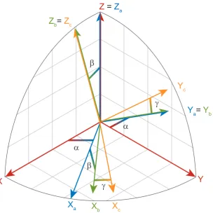
2.2 Rotation of a set of orthogonal axes specified by three Euler angles. . . 23

2.3 Chemical shift anisotropy powder pattern. . . 33

3.1 Absorptive and dispersive Lorentzian one-dimensional lineshapes. . . 40

3.2 Pulse sequence and coherence transfer pathway diagrams for a 2D NMR experiment. . . 42

3.3 Two-dimensional NMR line shapes. . . 44

3.4 Pulse sequence and coherence transfer pathway diagram for a 1H DQ correlation experiment. . . 47

3.5 Rotation of a sample relative to theB0 field in an MAS experiment. . . 51

3.6 Continuous phase profile of a DUMBO pulse. . . 55

3.7 Pulse sequence diagram illustrating windowed decoupling. . . 56

3.8 POST-C7 pulse sequence. . . 57

3.9 Selection rules for aC71₂ based recoupling sequence. . . 59

3.10 Pulse sequence and coherence transfer pathway diagram for the cross polarisation (CP) experiment. . . 61

3.11 Pulse sequence and coherence transfer pathway diagrams for a 1H DQ correlation experiment. . . 63

3.12 Schematic DQ correlation spectrum. . . 64

3.13 Pulse sequence and coherence transfer pathway diagrams for a 2D 1H– 13_{C refocussed INEPT experiment. . . .} ₆₅

4.1 1H DQ CRAMPS spectrum ofβ-AspAla . . . 73

4.2 Rows extracted from 2D1H DQ CRAMPS spectra of β-AspAla . . . 76

4.3 Experimental and Simulated1H DQ build-up curves forβ-AspAla . . . 78

4.4 Experimental and Simulated 1H DQ build-up curves for specific H–H interactions inβ-AspAla . . . 79

4.5 Experimental and Simulated 1H DQ build-up curves to investigate the dipolar truncation due to a CH2 group . . . 81

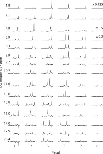
4.6 1H DQ build up curves: changing the number of simulated nuclei in comparison to experiment. . . 82 4.7 Simulated1H DQ build up curves: changing the 1H Larmor frequency . 84

(8)

4.8 Simulated1H DQ build up curves: changing the MAS frequency . . . . 85

5.1 Structural diagrams of sibenadet HCl . . . 89

5.2 13C CP MAS spectra of sibenadet HCl forms I and II . . . 92

5.3 Intermolecular interactions in sibenadet HCl form I . . . 94

5.4 30 kHz and 12.5 kHz (CRAMPS)1_{H one pulse spectra of sibenadet HCl} forms I and II . . . 96

5.5 1H DQ CRAMPS spectra of sibenadet HCl forms I II . . . 98

5.6 Intermolecular H–H proximities involving hydrogen-bonded protons in sibenadet HCl . . . 99

5.7 Row extracted from a1H DQ CRAMPS spectrum of sibenadet HCl form I, showing NH2–NH2 peaks . . . 100

5.8 Simulated and experimental 1H DQ build-up curves for NH–NH and NH–OH interactions in sibenadet HCl . . . 102

5.9 Experimental DQ build-up curves for sibenadet HCl forms I and II . . . 104

6.1 Molecular structure of indomethacin . . . 107

6.2 Pulse sequence, coherence transfer pathway diagram and schematic spec-trum for a1H(DQ)–13C(SQ) correlation experiment. . . 109

6.3 Supercell used to calculate the chemical shifts in an effectively isolated indomethacin molecule . . . 110

6.4 30 kHz and 12.5 kHz (CRAMPS)1H one pulse spectra ofγ-indomethacin112 6.5 13C CPMAS spectrum ofγ-indomethacin. . . 113

6.6 1_H–13_{C refocussed INEPT spectrum of} _{γ-indomethacin and structural} diagrams illustrating intermolecular interactions . . . 114

6.7 1H DQ CRAMPS spectrum ofγ-indomethacin . . . 116

6.8 Experimental and simulated1_{H DQ build-up curves for the OH–OH and} OH–Harom. interactions in γ-indomethacin . . . 118

6.9 The aromatic region of a1H(DQ)–13C(SQ) refocussed INEPT correlation spectrum ofγ-indomethacin . . . 121

6.10 Experimental and simulated1H DQ build-up curves for selected Harom.– Harom. interactions in γ-indomethacin . . . 124

7.1 Molecular structure of ibuprofen. . . 128

7.2 Unit cell diagrams of ibuprofen form II structures. . . 130

7.3 13C CP MAS spectrum of ibuprofen form I. . . 131

7.4 13C CP MAS spectra showing the emergence of ibuprofen form II as amorphous ibuprofen is annealed. . . 133

7.5 Comparison of the aliphatic and aromatic regions of the 13C spectra of ibuprofen forms I and II. . . 134

7.6 13C CP MAS spectra of ibuprofen forms I (as received and reconverted) and II. . . 136

(9)

I would like to thank my supervisor, Prof. Steven Brown, for giving me the opportunity to undertake an interesting and exciting research project and for the help and guidance he has provided throughout my PhD studies. I am also very grateful to the rest of the solid-state NMR group, especially those who have (very patiently) taught me how to use the spectrometers and resolved many technical problems for me.

I would also like to acknowledge the contributions of several people to the projects presented in this thesis, notably Les Hughes and Dave Martin, for their involvement in the sibenadet HCl project, and for allowing me to make use of the solid-state NMR facilities at AstraZeneca; Carmen Tripon and Claudiu Filip for their advice and as-sistance in the DQ simulations work and Oleg Antzutkin, for his involvement in the indomethacin project. Funding from AstraZeneca is gratefully acknowledged.

Many thanks to all of my friends, but in particular Ruth, who has been so kind and supportive, and has always cheered me up on days when the thesis writing was not going well. Finally I wish to thank my parents, my sister, Louise and the rest of my family, for their support and encouragement, not just during my PhD, but for all of the last twenty-six years.

(10)

DECLARATION

The work presented in this thesis is my own, except where stated otherwise in the text. The research was conducted under the supervision of Prof. Steven P. Brown at the University of Warwick between July 2007 and April 2011.

This thesis has not been submitted for a degree at another university.

Some of the results presented in this work, specifically those presented in chapter 4, have been published:

J. P. Bradley, C. Tripon, C. Filip and S. P. Brown. Determining relative proton-proton proximities from the build-up of two-dimensional correlation peaks in1_H

double-quantum MAS NMR: insight from multi-spin density matrix simulations. Phys. Chem. Chem. Phys., 11(32):6941–6952, 2009. [1]

(11)

The objective of the work presented in this thesis is to apply advanced high-resolution solid-state NMR methods for the structural characterisation of organic crystalline sys-tems, specifically active pharmaceutical ingredients (APIs). The determination of the crystal packing is an important stage in the development of new APIs, and solid-state magic angle spinning (MAS) NMR is well suited to complement existing techniques. Improvements in spectral resolution in recent years have led to the development of homonuclear correlation experiments capable of identifying intermolecular proximities between 1H nuclei. These experiments provide a powerful probe of the local environ-ment of each 1H nucleus in the three-dimensional structure, and the majority of the research presented in this thesis is focussed on the development of detailed analysis methods that may be used to extract more detailed structural information from 2D solid-state NMR correlation spectra.

Throughout this thesis, experimental solid-state NMR results are analysed along-side computational data, including density matrix simulations of experiments and first-principles calculations of shielding tensors. The results of simulations of a 1H DQ (double-quantum) correlation experiment are compared to experiment, in order to in-vestigate the dependence of the DQ build-up (change in peak intensity as a function of the recoupling pulse duration) on the precise nature of the dipolar coupled proton network. It is found (for a simple dipeptide) that quantitative information on the rel-ative H–H distance may be obtained by comparison of the maximum intensity reached in the corresponding1H DQ build-up curves. This method is then applied to pharma-ceutically relevant systems. It is shown that differences between two polymorphs of an API may be identified in the 1_{H DQ build-up of particular peaks, and, following the}

analysis for the dipeptide, this difference may be ascribed to differences in specific in-termolecular distances. In the study of a second API,γ-indomethacin, it is shown that the standard1_{H DQ experiment provides insufficient resolution to identify specific DQ}

peaks. A recently developed1H(DQ)–13C correlation experiment is used to exploit the higher resolution in the 13C dimension, hence allowing the extraction of DQ build-up curves which may be used, in conjunction with simulations, to obtain structural data. Finally, a recently discovered polymorph of the API ibuprofen is studied using

13_{C CPMAS (cross polarisation) solid-state NMR. Through the use of first-principles}

calculations, the13_{C spectra of both the well known and new polymorphs are assigned,}

and the conversion of an amorphous solid to the new polymorph is monitored through the use of temperature-controlled solid-state NMR experiments.

(12)

ABBREVIATIONS

ABMS Anisotropic Bulk Magnetic Susceptibility

API Active Pharmaceutical Ingredient

BABA BAck-to-BAck

CP Cross Polarisation

CRAMPS Combined Rotation And Multiple Pulse Spectroscopy

CSA Chemical Shift Anisotropy

DFT Density Functional Theory

DQ Double Quantum

DUMBO Decoupling Using Mind Boggling Optimisation

FID Free Induction Decay

FSLG Frequency-Switched Lee-Goldburg

FT Fourier Transform

FWHMH Full Width at Half Maximum Height

GIPAW Gauge-Including Projector Augmented Waves

INEPT Insensitive Nuclei Enhanced by Polarisation Transfer

MAS Magic Angle Spinning

NMR Nuclear Magnetic Resonance

PAS Principal Axis System

PMLG Phase-Modulated Lee Goldburg

ppm Parts Per Million

POSTC7 Permutationally Offset Stabilised C7

REDOR Rotational-Echo DOuble Resonance

rf Radio Frequency

S/N Signal-to-Noise

(13)

SQ Single Quantum

TPPI Time Proportional Phase Increment

TPPM Two Pulse Phase Modulated

(14)

CHAPTER

ONE

INTRODUCTION

1.1 Solid-State NMR Background

The field of nuclear magnetic resonance (NMR) has experienced an extraordinary pace of development since the first observations of NMR signals from bulk materials, in experiments performed independently by Purcell [2] and Bloch [3] and co-workers in 1946. It is notable that although some of the initial experiments by both Purcell and Bloch were performed on solid samples, the majority of the development in NMR for many years was focussed on liquids. A simple NMR experiment performed on a static solid sample will usually result in a broad featureless peak, due to the many anisotropic interactions present in a solid sample. Solution-state NMR is unencumbered of such considerations due to the rapid and essentially random molecular motion inherent to liquids, which results in an averaging of anisotropic interactions over an extremely short time-scale. Consequently, high resolution NMR spectra are readily obtainable from solutions and so the technique has become a routine analytical tool in many branches of chemistry.

Despite the inherent difficulty of performing NMR experiments on solid-state sam-ples, a wealth of information unobtainable by other spectroscopic techniques is poten-tially available if these problems can be overcome. For many practical applications, it is useful to study the solid, rather than a solution. For example, the work presented in later chapters of this thesis is principally concerned with the use of NMR to inves-tigate the way in which organic molecules pack together in the solid state. In order

(15)

to obtain useful information from an NMR spectrum of a solid sample, the resolu-tion of the spectrum must be improved. The most widely applied method to reduce the width of spectral lines in solid-state NMR is magic-angle spinning (MAS). This technique involves rapid rotation of the sample about an axis inclined at an angle of arctan√2 ≈54.7◦ relative to the externally applied magnetic field, which results in a partial averaging of the anisotropic interactions.

The use of MAS to improve the resolution of a solid-state NMR spectrum was first reported independently by Andrew et. al. [4, 5] and Lowe [6] in the late 1950s. The advancement in MAS technology has resulted in ever increasing spinning frequencies being achieved, with a corresponding decrease in the diameter of the rotor used to hold the sample [7]. While MAS at relatively low frequencies (of the order of several kilohertz) is sufficient to produce high resolution spectra for nuclei such as13C or15N, it is not effective in the removal of the very strong 1_H–1_{H or} 19_F–19_{F homonuclear}

dipolar coupling interactions. Consequently homonuclear decoupling techniques, which involve the application of high powered rf pulses to the sample, have been developed to provide an alternative method of line narrowing in solid-state NMR experiments on

1_{H or} 19_{F nuclei [8, 9].}

Early examples of homonuclear decoupling techniques were designed to be applied to static samples. In the mid-1960s Lee and Goldburg demonstrated the use of radio-frequency (rf) irradiation to narrow the19F lines in a sample of calcium fluoride. Their method involved the application of continuous, off-resonance rf to create an effective field aligned at the magic angle to the external field [10]. The precession of the nuclear magnetisation about this effective field resulted in an averaging of the first order dipolar Hamiltonian, and a corresponding decrease in the line width. An alternative approach was proposed three years later by Waugh and co-workers [11, 12]. Their method, again applied in the static case, involved the use of a series of on-resonance rf pulses of varying phase. The use of this sequence, designated WaHuHa or WHH, resulted in an averaging of the first and second order dipolar Hamiltonian terms. The introduction of WHH also marked the first use of windowed decoupling sequences. Since the sequence consisted of a series of rf pulses and delays rather than continuous irradiation, the NMR signal could be acquired during the delays.

(16)

1.1. SOLID-STATE NMR BACKGROUND 3

spectral lines as the homonuclear dipolar coupling is reduced, broadening due to the chemical shift anisotropy (CSA) remains. The emergence of combined rotation and multiple pulse spectroscopy (CRAMPS) [13–15], in which multiple pulse homonuclear decoupling schemes combined with physical rotation of the sample by MAS has there-fore led to further improvements in spectral resolution for 1_{H solid-state NMR.}

Ex-amples of commonly used CRAMPS sequences include frequency-switched [16] and phase-modulated [17] Lee-Goldberg sequences (FSLG and PMLG respectively) and the DUMBO (decoupling using mind boggling optimisation) [18] sequence. The DUMBO sequence and in particular the eDUMBO [19] variant, which is directly optimised through experiment, are used extensively in experiments presented in later chapters of this thesis, in both windowed and windowless forms.

While the discussion so far has focussed on the efforts to improve the spectral resolu-tion by removing the anisotropic interacresolu-tions that cause line broadening in a solid-state NMR experiment, a total removal of these interactions at all times during the course of an experiment is not always desirable. Indeed, rather than representing a lack of information, the broad featureless peak seen in a static experiment without decoupling on a solid sample can be thought of as far too much information being presented in the spectrum. The anisotropic chemical shift and dipolar coupling interactions that cause the broadening are dependent on the precise arrangement of nuclei in the solid-state. If this information can be selectively re-introduced into a high-resolution spectrum, it provides a powerful probe of the local chemical environment of each nuclear site in the sample.

(17)

magnitude of the dipolar coupling interaction depends on the internuclear distance to the inverse third power. It therefore provides an extremely sensitive measurement of the separation between the two nuclei. Experiments to measure the dipolar coupling between a pair of spins use rotor synchronised pulse sequences to recouple the interac-tion, re-introducing the dipolar coupling removed by magic angle spinning. In the case of heteronuclear couplings, pulse sequences such as REDOR (Rotational-echo double resonance) [24] may be used.

Much of the work presented in this thesis involves the use of the homonuclear dipolar interaction between coupled 1H nuclei to obtain structural information. A homonuclear approach to the measurement of the dipolar coupling is therefore required. This relies on the use of double-quantum (DQ) filtered experiments, which excite the DQ coherence between dipolar coupled nuclei [25]. Following the initial development of rotor synchronised sequences for the recoupling of the dipolar interaction [26, 27], a wide variety of different recoupling sequences have been introduced [28–31]. A two-dimensional experiment is required, since the DQ coherence is not directly observable. It must be allowed to evolve during an indirectly observed time dimension, before conversion to a single-quantum coherence which results in an observable NMR signal. DQ filtered experiments have been successfully used to measure the dipolar coupling, and hence distance, between pairs of 13C nuclei in selectively labelled compounds [32]. A simple two-dimensional DQ experiment will result in a spectrum showing correlation peaks for dipolar coupled nuclei at the isotropic chemical shift in one dimension, and at sums of chemical shifts in the other. Such a spectrum acts rather like a map of the nuclei within the sample, identifying which nuclei are in close spatial proximity.

The use of these experiments for1H nuclei was first reported in the mid-1980s [33], in studies of spin-clusters in deuterated materials. The increase in the available MAS rate led to the use of 1H DQ experiments combined with fast MAS to achieve spectra of natural abundance organic compounds, with sufficient resolution to identify DQ peaks due to specific dipolar-coupling interactions [34–36]. The addition of CRAMPS decoupling schemes during both t1 and t2 gave further increases in the resolution of 1_{H DQ spectra [37–39]. A striking example of the superior resolution provided by}

(18)

1.2. POLYMORPHISM AND PHARMACEUTICALS 5

(12.5 kHz MAS) spectrum of the dipeptideβ-AspAla, in contrast to widths of 1.5 ppm in a spectrum recorded at 30 kHz. Although recent advances in MAS technology have resulted in modern commercially available equipment capable of spinning frequencies in excess of 60 kHz, the resolution in1H DQ spectra of organic solids achieved through the use of such fast MAS still does not in general reach that for spectra acquired at lower spinning frequencies with the addition of homonuclear decoupling.

Recent years have seen an increasing use of computational techniques in conjunction with solid-state NMR experiments. Simulations are now regarded as an essential coun-terpart to experiment in the field of developing new solid-state NMR techniques [40]. Several numerical simulation software packages capable of accurately reproducing ex-perimental results are now freely available [41–43] and these have been used to study a wide variety of areas, including double-quantum build-up [1], spin-echo dephasing [44] and homonuclear [45] and heteronuclear [46, 47] decoupling techniques.

First principles calculations based on density functional theory (DFT) also play an important role in the investigation of crystal structures by solid-state NMR. The CASTEP [48] program uses plane-wave pseudopotentials [49] to describe the electron density throughout a material. The dependence of this method on periodic structure makes it ideally suited to the study of crystalline systems. CASTEP may be used to calculate a variety of properties of a crystalline system, including the optimum atomic positions and, through the use of the GIPAW (gauge including projector augmented waves) method [50, 51], the shielding effect due to electrons at each nuclear position, and hence the chemical shift. The GIPAW approach has been successfully implemented in the investigation of a wide range of systems in conjunction with solid-state NMR experiments [52–61]. Both density matrix simulations and DFT calculations have been used extensively in the work presented in this thesis to aid in the interpretation of solid-state NMR spectra.

1.2 Polymorphism and Pharmaceuticals

(19)

in profound variations in the physical properties of the bulk material. For example, it is easy to picture a situation whereby differences in the strength of intermolecular bonds between two polymorphs could result in significant differences in the melting point or solubility of the solid. The existence of multiple polymorphs of an organic molecular crystal, under normal pressure conditions is extremely common, with research suggesting that over one third of organic solids exhibit polymorphic behaviour [63].

The identification of polymorphs is possible by a variety of means including mi-croscopy, thermal analysis, density measurements and diffraction experiments. Single crystal x-ray diffraction in particular is an ideal technique to identify the differences in crystal structure which are, by definition, present between different polymorphs of the same molecule [62]. In contrast to diffraction techniques, solid-state NMR allows the study of the local environment of each nucleus, rather than long range order. Conse-quently, solid-state NMR has the potential to provide complementary information to other structural determination techniques. Solid-state NMR remains useful in situa-tions where a single crystal cannot be obtained, indeed a powdered sample is almost always preferable and the technique even remains applicable to amorphous solids [64]. There are numerous examples of studies of amorphous organic samples [65–67], al-though the spectra of such samples are likely to exhibit broader lines.

Solid-state NMR studies can reveal a wide variety of information useful in un-derstanding the crystallographic structure of an organic material. For example, the shielding interaction is sensitive to differences in intermolecular arrangements, hence differences between polymorphs can be identified based on changes in isotropic chem-ical shifts [68]. Different polymorphs of the same substance would not necessarily be expected to have the same number of distinct molecules in the asymmetric unit cell. This information is readily available in a relatively high resolution solid-state NMR spectrum, such as 13C CPMAS, of an organic solid. Peaks in such a spectrum will be split according to the number of distinct molecules, due to the slight differences in the local electronic environment. Solid-state NMR also offers the possibility of di-rectly investigating intermolecular interactions, such as hydrogen bonding, which would typically be expected to differ between polymorphs [62].

(20)

1.2. POLYMORPHISM AND PHARMACEUTICALS 7

solid-state NMR have involved the use of the CPMAS experiment, usually applied to

13_{C, although}15_{N studies are also reasonably commonplace [70, 71]. The reason for the}

predominant focus on these nuclei is the ease with which high resolution spectra can be obtained. Using only moderately fast MAS and heteronuclear decoupling, spectra of resolution approaching that obtained from solution-state experiments can be acquired; in many cases, the resolution is sufficient to clearly separate all peaks due to different nuclear sites. Due to the greater difficulty in obtaining spectra of sufficient resolu-tion, there has been considerably less use of 1H solid-state NMR in the investigation of polymorphism. However as a result of recent improvements in resolution due to fast MAS and homonuclear decoupling,1H solid-state NMR experiments have been used to differentiate between different solid forms of pharmaceutical products [72].

There are clear benefits to using 1H solid-state NMR in structural investigations of organic solids. Due to the high natural abundance, double-quantum correlation experiments can be performed in a relatively short time without the need for isotopic enrichment. These experiments have been used extensively to investigate intermolecular interactions in a variety of different systems [25, 35, 73–76]. It is therefore clear that the 1H DQ solid-state NMR experiment has the potential to provide new insight into the investigation of polymorphic systems.

In the context of the pharmaceutical industry, where a large number of drugs are prepared in the form of solid tablets, polymorphism is a central concern at all stages in the design and manufacture of a drug product. Different polymorphs of an active pharmaceutical ingredient (API) may exhibit considerable differences in a wide variety of physical and chemical properties, many of which have the potential to significantly influence the performance of the drug product. There are numerous examples in the literature of cases where the bioavailability of an API, predominantly determined by the solubility and dissolution properties [62], differs between solid forms [77–80].

(21)

case is that of the API ranitidine hydrochloride. A dispute arose between the original manufacturer, Glaxo Group (now Glaxo SmithKline), and a manufacturer of generic drugs over the question of which of two known polymorphs were produced by the pro-cess described in the original patent [81]. The case was settled in Glaxo’s favour only after analysis of the product produced by the process indicated that only the correct polymorph could be produced, in the absence of seed crystals of the other polymorph. For reasons such as those outlined above, the identification and characterisation of polymorphs, and the control of the polymorph produced during drug manufacture, is of critical importance to the pharmaceutical industry. A number of analytical techniques can be used for this purpose, and it is clear that solid state NMR has the potential to play a key role. Although there is already reasonably widespread use of relatively simple experiments such as13C CPMAS, the combination of these with more advanced homo- and hetero-nuclear correlation experiments, and first principles calculations, will lead to a greater understanding of the structure and properties of a wider variety of polymorphic systems. The purpose of this thesis is to present such novel solid-state NMR techniques for the investigation of the structural properties of organic solids, with particular emphasis on the identification and characterisation of polymorphic forms, and to demonstrate their application to real pharmaceutical systems.

1.3 Thesis Overview

(22)

1.3. THESIS OVERVIEW 9

techniques used to probe these interactions and hence extract useful information. Sev-eral pulse sequences using these techniques are then presented. Finally there is a short discussion of computational methods used in the analysis and interpretation of the experimental results.

Chapter four presents the results of density matrix simulations of a1_{H DQ}

exper-iment, applied to small clusters of nuclei, with positions extracted from the crystal structure of the dipeptide β-AspAla. The dependence of the DQ peak intensity on the duration of the recoupling sequence was investigated, and the corresponding DQ build-up curves compared to those obtained from DQ CRAMPS experiments. It was found that the DQ build-up behaviour for a particular interaction is strongly influenced by the associated internuclear distance, even within a dense network of strongly coupled spins. Chapter five shows the application of the DQ build-up experiments investigated in the previous chapter to the study of two polymorphs of an active pharmaceutical ingredient. Density functional theory (DFT) calculations are used to optimise a crystal structure and calculate chemical shift values, which are used in assigning the high ppm 1H peaks due to hydrogen-bonded protons. The similarity in the 1H DQ CRAMPS spectra of two polymorphs indicates the same intermolecular hydrogen bonding arrangement, however subtle differences in the1H DQ build-up behaviour of peaks corresponding to intermolecular interactions indicate small differences in the intermolecular packing.

Chapter six presents an NMR crystallography study of the gamma polymorph of the API indomethacin. DFT calculations are performed, both to aid in the assignment of the1_{H and}13_{C solid-state NMR spectra, and to investigate the effects of}

intermolec-ular interactions on the 1H chemical shifts by performing calculations for an isolated molecule. The 1H DQ CRAMPS spectrum is shown to be of limited value in terms of 1H DQ build-up analysis, due to the inability to resolve peaks due to individual H–H interactions, except those involving the single hydrogen bonded proton. Conse-quently a 1H(DQ)–13C(SQ) refocussed INEPT correlation spectrum is used to transfer magnetisation from protons involved in homonuclear DQ coherences to directly bonded

13_{C nuclei. The resulting spectrum enables individual peaks in the aromatic region to}

be resolved, and consequently 1_{H DQ build-up curves for individual} 1_{H nuclei may be}

extracted.

(23)

DFT calculations on two polymorphs of ibuprofen. Using calculated chemical shift val-ues for geometry optimised structures of both the well-known, pharmaceutically used form, and a recently discovered polymorph formed by annealing amorphous ibuprofen,

13_{C solid-state NMR spectra of both polymorphs are fully assigned. Variable}

(24)

CHAPTER

TWO

SOLID-STATE NMR THEORY

A solid-state NMR experiment is able to provide detailed atomic-level structural in-formation on a sample by probing the interactions experienced by a system of nuclear spins. In order to understand and properly interpret the results of such experiments, it is necessary to introduce the underlying quantum mechanics describing the behaviour of systems of nuclear spins. This chapter discusses the theory of nuclear magnetism in relation to NMR, and applies this to describing the internal interactions, such as the chemical shift and dipolar coupling, which are probed during an NMR experiment, and the external interactions which allow this information to be obtained. The material pre-sented in this chapter follows the theory and derivations prepre-sented in references [82–84].

2.1 Nuclear Magnetism

Nuclear magnetic resonance spectroscopy is concerned with the measurement of the precession frequencies of nuclear spins in a magnetic field. Through the use of com-plex sequences of radio-frequency (rf) pulses to manipulate interacting nuclear spins, detailed localised information can be obtained. Although simple NMR experiments on systems consisting of a number of non-interacting spin-½nuclei can be visualised using an intuitive model of rotations of the bulk nuclear magnetism within a sample, this approach is not sufficient to understand complex experiments involving many coupled nuclei. An approach based on a quantum mechanical model of nuclear magnetism is therefore required.

(25)

2.1.1 Spin Angular Momentum

Spin angular momentum is an intrinsic property of each nuclear isotope, and takes on discrete values of integer, or half-integer multiples of ¯h. The magnetic moment of the nucleus is directly proportional to the nuclear spin. Considering a single, isolated atomic nucleus, with non-zero spin, in an externally applied, static magnetic field, the energy of the spin is described by the Zeeman Hamiltonian, ˆH which is given by

ˆ

H =−µˆ·B0 (2.1)

whereB0is the applied magnetic field andµˆis the nuclear magnetic moment operator, which can be defined in terms of the spin angular momentum operator, Iˆ

ˆ

µ=γIˆ (2.2)

whereγ is the gyromagnetic ratio, a constant for each nuclear isotope. By convention, the direction of the external field is aligned along thezdirection. Due to this convention,

z is commonly referred to as the longitudinal direction, with x and y referred to as transverse. Applying this convention, equation 2.1 therefore becomes

ˆ

H =−γIˆzB0

=ω0Iˆz (2.3)

where ˆIz is the z- component of Iˆand the angular frequency, ω0, is the Larmor

fre-quency, which is related to the strength of the applied magnetic field by the gyromag-netic ratio.

ω0 =−γB0 (2.4)

It is possible to construct a wavefunction,|ψi, which completely describes all prop-erties of an atomic nucleus. For an NMR experiment, the property of interest is the nuclear spin. To determine the spin properties of a nucleus, the wavefunction is acted upon by the spin angular momentum operator,Iˆ. For a single nuclear spin, the opera-tor, ˆI2_{, which describes the magnitude of the nuclear spin angular momentum, and ˆ}_I

x,

ˆ

(26)

2.1. NUCLEAR MAGNETISM 13

related by the equation

ˆ

I2 = Î_x2+ Î_y2+ Î_z2 (2.5)

The ˆI2operator commutes with the operator for only one component of the spin angular momentum, by convention, the ˆIz operator. More specifically, the following

commuta-tion relacommuta-tions apply:

[ ˆI2,Iˆz] = 0 (2.6)

[ ˆIx,Iˆy] =i¯hIˆz (2.7)

where ¯h is the reduced Planck constant (h/2π). The commutation relations for other combinations of the Cartesian spin angular momentum operators are provided by sub-sequent cyclical permutations. These single spin angular momentum operators may also be expressed as 2×2 matrices:

ˆ Ix =



 

0 1₂

1 2 0



 ,

ˆ Iy =i



 

0 −1₂

1 2 0



 ,

ˆ Iz =



 

1 2 0

0 −1₂ 



 (2.8)

The ˆI2 and ˆIz operators have eigenvalues,I and m, respectively:

ˆ

I2 |ψi= ¯hI(I+ 1)|ψi (2.9) ˆ

Iz |ψi= ¯hm|ψi (2.10)

The valueI(I+1) is the square of the magnitude of the nuclear spin angular momentum, and m is its z component. The factor of ¯h is commonly omitted such that angular momenta are expressed in units of ¯h; this convention will be followed from here on.

(27)

as “spin up” for m= +1/2, denoted|αi, and “spin down” form=−1/2, denoted|βi.

ˆ

Iz|αi= +

1

2|αi (2.11)

ˆ

Iz|βi=−

1

2|βi (2.12)

By combining the above expressions with equation 2.3, the energies of spins in each of the Zeeman eigenstates can be found to be

ˆ

H|αi= +1

2ω0|αi (2.13)

ˆ

H|βi=−1

2ω0|βi (2.14)

showing that the separation in energy between the|αi and|βi eigenstates is equal to the Larmor frequency,ω0.

An isolated spin-½ nucleus need not necessarily exist purely in either eigenstate. In order to fully describe the spin state of the nucleus, a superposition of the Zee-man eigenstates must be used. The contributions of each of the basis states to the wavefunction is governed by the complex coefficients cα and cβ.

|ψi=cα|αi+cβ|βi (2.15)

where the normalisation condition |cα|2+|cβ|2 = 1 applies.

A generalised operator, ˆA, can be represented as a matrix, where hr|Aˆ|si forms the element Ars:

A= 

 

Aφ1φ1 Aφ1φ2 Aφ2φ1 Aφ2φ2

  =   

hφ₁|Aˆ|φ₁i hφ₁|Aˆ|φ₂i hφ₂|Aˆ|φ₁i hφ₂|Aˆ|φ₂i





 (2.16)

For the case of an operator, ˆA acting on a spin-½ nucleus, the expectation value of ˆA may therefore be expressed as a matrix multiplication

hAiˆ =

c∗_α c∗_β



 

Aαα Aαβ

Aβα Aββ

      cα cβ   

(28)

where the wavefunctions |ψi and hψ|have been expressed as column and row vectors respectively, the elements of which are the coefficients of the wavefunction’s eigenstates. The expectation value of the operator ˆIz operating on|ψimay therefore be expressed

as

hIˆzi=hψ|Iˆz |ψi

= 1 2(cαc

∗

α−cβc∗β)

= 1 2|cα|

2₋1

2|cβ|

2 _(2.18)

The values of |c_α|2 _and _|c

β|2 therefore correspond to the probability of a measurement

of the nuclear spin in the z-direction returning a value of +1/2 or −1/2 respectively. As implied by the commutation relations expressed in equations 2.6 and 2.7, the operators ˆIx and ˆIy do not share the|αi and |βi eigenstates. The effect of these

operators is to convert between|αi and|βi

ˆ Ix|αi=

1

2|βi (2.19)

ˆ Ix|βi=

1

2|αi (2.20)

ˆ Iy|αi=

1

2i|βi (2.21)

ˆ

Iy|βi=−

1

2i|αi (2.22)

The expectation values of the transverse spin angular momentum operators are also expressed in terms of the coefficients cα andcβ.

hIˆxi=

1 2(cαc

∗

β+cβc∗α) (2.23)

hIˆyi=

1 2i(cαc

∗

β−cβc∗α) (2.24)

2.1.2 Density Operator Theory

The expression for the expectation value in equation 2.17 shows that the expectation values of ˆAare comprised of the products of the coefficientscα andcβ. This can also be

(29)

matrix, ρ as ρ=    cα cβ    c∗_α c∗_β

=



 

cαc∗α cαc∗_β

cβc∗α cβc∗_β





 (2.25)

Taking the product of the density matrix and A produces a matrix with terms of the form cαc∗αAαα such as those that appear in the expectation value of ˆA

ρA= 

 

cαc∗α cαc∗_β

cβc∗α cβc∗_β

     

Aαα Aαβ

Aβα Aββ

   =   

cαc∗αAαα+cαc∗_βAβα cαc∗αAαβ+cαc∗_βAββ

cβc∗αAαα+cβc∗βAβα cβc∗αAαβ+cβc∗βAββ





 (2.26)

Inspection of the above matrix reveals that the terms in the expectation value of ˆA lie on the principal diagonal. The expectation value may therefore be found by taking the trace of the matrix

hAiˆ = Tr(ρA) (2.27)

The above description of the density matrix is limited to the case of a single

spin-½ nucleus, however the power of the density matrix formalism lies in the ability to describe large systems comprised of many nuclear spins. In a more general case, the density operator, ˆρ, may be defined as

ˆ

ρ= |ψihψ| (2.28)

where the overbar signifies an ensemble average over the entire system under consid-eration. The corresponding density matrix consists of elements ρrs defined in terms of

the density operator, as in equation 2.16:

ρrs=hr|ρˆ|si (2.29)

(30)

described in equation 2.15. The coefficientscα and cβ may be expanded in terms of an

amplitude, aand a phase, φ:

|ψi=aαeiφα|αi+aβeiφβ|βi (2.30)

The density matrix describing the system is therefore

ρ= 

 

aαa∗α aαa_β∗ei(φα−φβ)

aβa∗αei(φβ−φα) aβa∗_β





 (2.31)

For simplicity of notation, the overbars will be omitted in subsequent expressions, where the density operator and its matrix representation, the density matrix, will always be used to describe ensemble averages. Examining the density matrix in the above expression, and comparing to the expectation values of Îz, Îx and Îy in equations

2.18, 2.23 and 2.24 it is clear that the elements on the principal diagonal of the density matrix correspond to the expectation values of the ˆIz operator. These are known as the

populations of the|αi and|βi states. Similarly, the off-diagonal elements are related to the expectation values of the ˆIx and ˆIy operators. The phase dependence of these

terms is such that if the phases of the individual spin systems comprising the ensemble are the same, then eiφα−φβ _{will in general have some non-zero value, and a coherence}

will exist between the systems. Conversely, if the values of the phases are random, over the ensemble average the value ofeiφα−φβ _{will be zero and therefore no coherence will}

exist. These off diagonal elements are therefore referred to as coherences.

The density matrix representation of a spin system is easily expanded to accommo-date systems comprised of coupled spins. A dipolar coupled spin pair may be described by a wavefuntion with eigenstates such as|ββi (both spin-down) analogous to the eigenstates of an isolated spin-½nucleus in equations 2.11 and 2.12. The wavefunction may be expressed in terms of the corresponding eigenvalues cαα,cαβ,cβα and cββ:

|ψi= 

       

cαα

cαβ

cβα

cββ



       

(31)

|αα> |ββ>

|αβ> |βα> Energy m = 0

m = -1 m = +1

(a) (b)

SQ DQ

ZQ

Figure 2.1: (a) energy level diagram for a system comprised of two coupled spin-½ nuclei. (b) graphical representation of zero-quantum (black), single-quantum (red) and double-quantum (blue) coherences in a coupled spin-½pair.

These states may be represented as an energy level diagram, with theαβ andβαstates degenerate, as shown in figure 2.1(a).

The density matrix describing an ensemble of coupled spin-½ pairs is therefore

ρ=|ψihψ|

= 

       

cααc∗αα cααc∗αβ cααc∗βα cααc∗ββ

cαβc∗αα cαβc∗αβ cαβc∗βα cαβc∗ββ

cβαc∗αα cβαc∗αβ cβαc∗βα cβαc∗ββ

cββc∗αα cββc∗αβ cββc∗βα cββc∗ββ



       

(2.33)

The principal diagonal terms (cααc∗αα, cαβc∗αβ etc.) again correspond to the

popula-tions of the individual eigenstates of the coupled system. The remaining terms are coherences linking these states. The coherences are classified according to the differ-ence in the quantum number, m, of the states they link. Consequently cαβc∗_βα and

its complex conjugate cβαc∗_αβ are described as zero-quantum coherences, cααc∗_ββ and

cββc∗_ββ as double-quantum coherences and the remaining terms as single-quantum

co-herences. A graphical representation of these terms on an energy level diagram for a two-spin system is shown in figure 2.1(b). In comparison with the density matrix for an ensemble of isolated spin-½nuclei in equation 2.31, it is notable that a system of two (or more) coupled spin-½ nuclei is required for a double-quantum coherence to exist. The double-quantum coherence may therefore be probed to investigate the spin–spin interactions in a system.

(32)

2.1.3 Evolution of the Density Operator

Since the density matrix represents a complete description of the nuclear spin system, it provides a convenient way of following the evolution of such a system under a Hamil-tonian. This permits the calculation of the state of a nuclear spin system at any stage of an NMR experiment, providing Hamiltonians for all relevant interactions are known.

Differentiating the density operator with respect to time gives

d ˆρ(t) dt =

d

dt(|ψihψ|) =

d dt |ψi

hψ|+|ψi

d dthψ|

(2.34)

The time dependent Schr¨odinger equations for|ψi and hψ|are

d

dt |ψi=−iHˆ |ψi (2.35) d

dthψ|=ihψ| ˆ

H (2.36)

Substitution of these expressions into equation 2.34 gives:

d ˆρ(t) dt =−i

ˆ

H |ψihψ|+i|ψihψ|Hˆ =−ihH,ˆ ρ(t)ˆ

i

(2.37)

This is known as theLiouville-von Neumann equationand may be solved subject to the approximation that the Hamiltonian is constant with respect to time. In practice, this is a valid assumption provided that the Hamiltonian is considered over a small time interval, dt. Under conditions of a time-constant Hamiltonian, the solution to the Liouville-von Neumann equation is:

ˆ

ρ(t) =e−iHtˆ ρ(0)eˆ iHtˆ

= ˆU(t) ˆρ(0) ˆU(t)−1 (2.38)

(33)

in the above expression becomes

ˆ

ρ(t) = ˆT e−iR0tHtˆ

0_d_t0

ˆ

ρ(0)eiR0tHtˆ

0_d_t0

(2.39)

where the Dyson time ordering operator, ˆT, is required in situations where ˆH does not commute with itself at different times.

2.1.4 Product Operators

Product operators provide an alternative method of describing NMR experiments [85]. While the use of product operators is limited to situations of weak coupling, this remains useful for describing experiments which exploit theJ-coupling interaction.

In the case of a single spin system, the operators Îx, Îy and Îz, corresponding to

the x, y, and z magnetisation of a single spin respectively (expressed in matrix form in equation 2.8), suffice to describe the experiment in a manner equivalent to a simple vector model. In a system of two coupled spins,I andS(which may describe either like or unlike nuclei), the matrix representations of the Îx, Îy and Îz operators are found

by taking the direct product of the matrices for a single-spin system (equation 2.8) and the identity matrix. For ˆIx:

ˆ Ix =



 

0 1₂

1 2 0   ⊗    1 0 0 1   =         

0 0 1₂ 0 0 0 0 1₂

1

2 0 0 0

0 1₂ 0 0          (2.40)

Similarly for ˆIy and ˆIz:

ˆ Iy =

        

0 0 −1 2i 0

0 0 0 −1 2i 1

2i 0 0 0

0 1₂i 0 0         

, Iˆz=

         1

2 0 0 0

0 1₂ 0 0 0 0 −1

2 0

0 0 0 −1₂          (2.41)

The corresponding S spin operators may be similarly found by reversing the order of the direct product. It is notable that the ˆIz operator contains elements only on the

(34)

2.2. SOLID-STATE NMR INTERACTIONS 21

operators contain only off-diagonal elements, corresponding to the coherences linking those states.

The power of the product operator approach lies in the creation of two-spin opera-tors describing coupled systems. These operaopera-tors are formed from the products of the single-spin operators. Under the influence of a J coupling between two spin-½ nuclei (JIS), the ˆIx operator evolves with time as:

ˆ

Ix→Iˆxcos(πJISt) + 2 ˆIySˆzsin(πJISt) (2.42)

i.e., evolution under the J-coupling interaction results in magnetisation being created on the S spin, from an initial state in which magnetisation exists only on the I spin. This transfer of magnetisation is exploited in experiments such as INEPT, which will be discussed in chapter 3.

2.2 Solid-State NMR Interactions

In a solid-state NMR experiment, it is necessary to consider interactions both between the nuclear spin system and the external environment, and between multiple nuclear spins. The external interactions due to the applied magnetic fields are the methods used to probe or manipulate the internal interactions, which provide useful information on the sample.

2.2.1 Interaction Hamiltonians

The total nuclear spin Hamiltonian, ˆHtotal is comprised of components due to the

interactions with external fields, and internal spin–spin interactions. These components can then be broken down further into contributions from the specific interactions

ˆ

Htotal= ˆHext.+ ˆHint.

= ˆHZ+ ˆHrf+ ˆHσ+ ˆHD+ ˆHJ+ ˆHQ (2.43)

where ˆHZ and ˆHrf are the external interactions (Zeeman and rf pulses, respectively)

and the ˆHσ, ˆHD, ˆHJ and ˆHQ terms represent the internal interactions (respectively:

(35)

It is clear from the above that if appropriate Hamiltonians can be formulated for all interactions present in the system, the evolution of the density operator can be followed using the method presented in the previous section.

The general form for the Hamiltonian of a particular interaction, ˜A, is

ˆ

HA= ˆIA˜Sˆ

=

ˆ

Ix Iˆy Iˆz

     

Axx Axy Axz

Ayx Ayy Ayz

Azx Azy Azz

            ˆ Sx ˆ Sy ˆ Sz       (2.44)

where ˜A is a second rank tensor describing the interaction, ˆI is a spin operator and ˆS may be either a second spin operator, or an operator representing an external field.

For each interaction, a principal axis system (PAS) can be defined, such that the interaction tensor is diagonal. Hence the interaction Hamiltonian in the PAS, ˆH_AP, is

ˆ

H_AP = ˆIA˜PSˆ

=

ˆ

Ix Iˆy Iˆz

     

Axx 0 0

0 Ayy 0

0 0 Azz

            ˆ Sx ˆ Sy ˆ Sz       (2.45)

This principal axis system is useful when describing individual interactions; however, tensors of different interactions do not, in general, share the same PAS. For example, in the case of the dipolar coupling the PAS is defined by the internuclear vector, whereas the PAS of the shielding tensor depends on the electronic environment.

In NMR experiments, it is often necessary to consider multiple frames of reference, and to be able to transform between these frames, for example, transforming from the PAS of a dipolar coupling interaction to the lab frame.

2.2.2 Rotations: Euler Angles and Spherical Tensors

(36)

2.2. SOLID-STATE NMR INTERACTIONS 23

X

Y

X

_a

Y

_a

=

Y

_b

X

_b

X

_c

Y

_c

α

β

γ

α

β

γ

Z

_b

=

Z

_c

[image:36.595.184.489.71.376.2]

Z =

Z

_a

Figure 2.2: Rotation of a set of orthogonal axes (X,Y,Z) through Euler anglesα,β and γ. The figure shows each stage of the rotation (colour coded). Initial axes are shown in red followed by blue (one rotation), green (two rotations) and yellow (three rotations -final axes). Grey grid lines are aligned to the initial axes.

rotations about different axes. The rotation,R is expressed as

R(α, β, γ) =Rz(α)Ry(β)Rz(γ) (2.46)

This expression describes the three rotations necessary to move between any two frames. Considering an “intial” set of three axes X, Y, and Z, the first rotation is about the Z axis by an angleα. This creates a new set of axes,Xa,Ya andZa. A rotation about

the Ya axis by an angle of β is then performed, resulting in axes Xb, Yb and Zb. The

final rotation is by an angle ofγ about theZb axis, giving the finalXc,YcandZcaxes.

A graphical representation of the rotation of a set of axes through a set of Euler angles is shown in figure 2.2.

(37)

interaction Hamiltonians in terms of spherical tensors.

ˆ H=

2

X

j=0 +j

X

m=−j

(−1)mAjmTˆj−m (2.47)

where the tensors Ajm and ˆTj−m are the spatial and spin components of the

Hamil-tonian, respectively. Changes to the reference frame due to rotations affect only the spatial components. The subscripts j and m refer to the rank of the tensor and the order of the tensor component, respectively. From the limits imposed on the values of j and m, it is clear that there are nine possible spatial spherical tensors. These tensors can be expressed in terms of the components of the Cartesian tensors, and will be defined as such when necessary.

It is, however, notable that the spherical tensors A00, A20 and A2±2 are the only

spatial spherical tensors to have a dependence on the diagonal elements of A, therefore only these four components can appear in the equation for the Hamiltonian in the PAS:

ˆ

H_AP AS =AP AS₀₀ Tˆ00+AP AS20 Tˆ20+AP AS22 Tˆ2−2+AP AS2−2 Tˆ22 (2.48)

The primary advantage of working with spherical tensors comes when moving be-tween reference frames using a rotational transformation. The rank of a spherical tensor is invariant under rotation - this feature greatly reduces the complexity of performing such an operation. In general, a tensor Ajm is converted into a sum of tensors of the

same rank, but of different orders

R(Ajm) =

+j

X

m0₌₋_j

D_mj 0_m(α, β, γ)A_jm0 (2.49)

where the terms Dj_m0_m(α, β, γ) are the Wigner rotation matrices. This shows that

a rotation operation may be simplified to a matrix multiplication involving only the spatial spherical tensors. TheDj_kl(α, β, γ) terms may be defined in terms of the reduced Wigner rotation matrix elements, dj_kl(β), which are trigonometric functions:

D_klj (α, β, γ) = exp(−ikα)dj_kl(β) exp(−ilγ) (2.50)

(38)

2.3. INTERACTIONS WITH EXTERNAL FIELDS 25

of Euler angles linking the PAS to the lab frame:

ˆ ALAB_jm0 =

+j

X

m=−j

Dj_mm0(αP L, βP L, γP L)APASjm (2.51)

2.2.3 High Field Approximation

The expression for an interaction Hamiltonian in terms of spherical tensors in equation 2.47 may also be simplified by applying the high field, or secular, approximation. This approximation relies on the large magnitude of the externally applied magnetic field, resulting in the Zeeman Hamiltonian being the dominant term in equation 2.43. First order perturbation theory may then be applied:

ˆ

HTotal= ˆH0+ ˆH1 (2.52)

where

ˆ

H0= ˆHZ

ˆ

H1= ˆHrf+ ˆHσ+ ˆHD+ ˆHJ+ ˆHQ (2.53)

i.e., the non-Zeeman interactions are treated as perturbations to the Zeeman Hamilto-nian. From this approximation, it follows that the eigenfunctions of the perturbation must be eigenfunctions of the Zeeman Hamiltonian. This allows the simplification of the Hamiltonian, as the only terms that will contribute to the spin energy levels are those that commute with the Zeeman Hamiltonian. More specifically, the following commutation relation applies:

h ˆ Iz,Tˆjm

i

=mTˆjm (2.54)

This relation shows that only when m= 0 will the commutator equal zero.

2.3 Interactions With External Fields

(39)

application of rf pulses. Considering first the interaction with the B0 field, the initial state of the system, before the application of anyrf pulses, can be described by finding the density operator at thermal equilibrium.

2.3.1 Zeeman Interaction

The Zeeman interaction is the interaction between a nuclear spin and the external static magnetic field. When expressed in the manner presented in equation 2.44, the Zeeman interaction Hamiltonian (for a magnetic field aligned along thez-axis) is:

ˆ

HZ = ˆIZ˜Bˆ

=−

ˆ

Ix Iˆy Iˆz

γ      

1 0 0 0 1 0 0 0 1

            0 0 B0      

=ω0Iˆz (2.55)

This gives the same result previously stated in equation 2.3 (except the now omitted factor of ¯h). From this equation it follows that the equilibrium density operator is:

ρeq=

e−βω0Iˆz

Tre−βω0Iˆz

(2.56)

where kB, the Boltzmann constant and T, the temperature, are contained in the term

β = 1/kBT. In the case of high temperatures (in this case “high temperature” means

any value of T above a very small fraction of a Kelvin, thus this is in practice always the case for NMR experiments), the approximations β 1, and en ≈ 1 +n may be applied. The above expression is now simplified to:

ρeq =

1 Tr(1−βω0Iˆz)

− βω0 Tr(1−βω0Iˆz)

ˆ

Iz (2.57)

= 1 Tr(1)−

βω0

Tr(1) ˆ

(40)

2.3. INTERACTIONS WITH EXTERNAL FIELDS 27

which, given that Tr(1) = 2N for a system ofN spins, and assuming N is very large, gives the density operator at thermal equilibrium as

ρeq ∝Iˆz (2.59)

Hence the density matrix only contains terms on the principal diagonal, i.e. only terms corresponding to the populations of the Zeeman eigenstates. This is an important result as this state of thermal equilibrium is assumed at the start of an experiment. This is a valid assumption provided sufficient time is allowed between successive experiments to allow the system to relax back to this state.

2.3.2 Radio-Frequency Pulses

In order to create coherences, a pulse (or series of pulses) of current oscillating at a frequency close to ω0, referred to as an rf pulse, is passed through a coil wrapped

around the sample. This generates a magnetic field in the transverse plane, B1(t). Although this field is typically much weaker than theB0 field, it can still have a strong

effect on the nuclear magnetisation if it is a resonant pulse, i.e., ωrf is close to ω0.

The form of theB1(t) magnetic field during the duration of the pulse is (assuming a pulse oscillating along the x-direction):

B1(t) =i2B1cos(ωrf t+φ) (2.60)

where i is the unit vector aligned along the x-axis. This oscillation may be broken down into two components, at frequencies ±ωrf

B1(t) =iB1

ei(ωrft+φ)₊_e−i(ωrft+φ)

(2.61)

Only one of these components (by convention +ωrf) is considered, as the−ωrfterm will

be so far off resonance as to have no significant effect on the nuclear spin.

NMR experiments are considered in the rotating frame, in which thex and y axes precess about the z axis at a frequency equal to ωrf. In practice, this corresponds to

(41)

than ωrf (kHz rather than hundreds of MHz). This process therefore has a practical

purpose, as these lower frequencies are easier for the spectrometer hardware to digitise. Considering a pulse inducing a magnetic field along thex-axis (a pulse of phasex) the Hamiltonian, in the rotating frame, ˆHrf for this pulse is

ˆ

Hrf =ω1Iˆx (2.62)

where ω1 is the nutation frequency,ω1=−γB1, i.e. the frequency at which the pulse

rotates the magnetisation about the x-axis (in this case). The evolution of the density operator under the effect of this pulse may be followed using the Liouville von-Neumann equation. The propagators formed from the above Hamiltonian may be expressed as matrices using the relation

e±iω1tIˆx ₌



 

cos 1₂ω1t

±isin 1₂ω1t

cos 1₂ω1t





 (2.63)

Assuming the system starts at thermal equilibrium, ˆρ= ˆIz, and evolves only under the

influence of therf pulse, the density matrix has the following form:

ˆ

ρ(t) =e−iHtˆ ρ(0)eˆ iHtˆ

= 

 

cos 1₂ω1t

−isin 1₂ω1t

cos 1₂ω1t

      1 2 0

0 1₂      

cos 1₂ω1t

isin 1₂ω1t

cos 1₂ω1t

   = 1 2   

cos (ω1t) isin (ω1t)

−isin (ω1t) −cos (ω1t)





 (2.64)

Inspection of the above expression shows that in the specific case where ω1t = π/2

(a “90◦” pulse), the population terms go to zero, while the coherence terms become non-zero. Similarly for a 180◦ pulse (ω1t=π), the populations are inverted.

2.3.3 Resonance Offset and Detection

Finally, it is necessary to discuss the evolution of the density operator under the influ-ence of a resonance offset, Ω =ω0−ωrf.

(42)

magneti-2.3. INTERACTIONS WITH EXTERNAL FIELDS 29

sation, immediately following a 90◦ pulse, i.e. ˆρ= ˆIx. The Hamiltonian describing the

evolution is

ˆ

HΩ = Ω ˆIz (2.65)

In a similar manner to that previously used to calculate ˆρ(t) for evolution under anrf

pulse, the solution to the Liouville von-Neumann equation can be found:

ˆ ρ(t) = 1

2 

 

0 e−iΩt eiΩt 0





 (2.66)

This result shows that under a resonance offset, the coherence terms of the density matrix oscillate at a frequency Ω.

In an NMR experiment, the technique of quadrature detection is employed, in which signals are acquired in two orthogonal directions (xandy) within the transverse plane. This method of detection is equivalent to acting on the density matrix with the raising operator, defined as:

ˆ

I+= ˆIx+iIˆy

=    0 1 0 0    (2.67)

Using equation 2.27, the expression for the expectation value of an operator, the form of the NMR signal, s(t) can be found by evaluating the trace of the product of the raising operator and the density operator for the system as it evolves under an offset:

s(t) = Tr( ˆI+ρ)ˆ

= Tr       0 1 0 0      

0 e−iΩt eiΩt ₀

      = 1

2(cos(Ωt) +isin(Ωt)) (2.68)

(43)

plane it is clear that these signals correspond to the signals in orthogonal directions. This expression for the NMR signal neglects the loss of transverse magnetisation due to relaxation mechanisms.

2.4 Internal Interactions

In addition to the interactions described in the previous section between the nuclear spin system and externally applied magnetic fields, there are also interactions with mag-netic fields inside the sample, either between nuclei and electrons, or between multiple nuclei. Without the presence of these interactions, an NMR spectrum would simply comprise a single peak at the Larmor frequency of the nuclear species being studied, however, by exploiting these interactions, it is possible to gain access to a large amount of chemical and structural information. The interactions relevant to experiments de-scribed in later chapters are the chemical shielding, the dipolar coupling and the J

coupling. These interactions will be described in individual sub-sections below. The quadrupolar coupling is also relevant in many NMR experiments, although not so in the context of the work presented in this thesis, as all experiments were performed on spin-½ nuclei, which do not have an electric quadrupole moment and hence do not couple to the electric field gradient. Therefore there will be no further discussion of the quadrupolar interaction.

2.4.1 Chemical Shift

(44)

2.4. INTERNAL INTERACTIONS 31

In practice, the frequency at which a peak appears in an NMR spectrum is expressed as a chemical shift which is defined relative to a reference frequency. The isotropic chemical shift,δiso, is defined in terms of the measured frequency, ω, and the reference

frequency, ωref, as:

δiso=

ω−ωref

ωref

×106 (2.69)

The factor of 106 _{is required to express the chemical shift in term of parts per million}

(ppm) of ωref. Expressing the frequency in this way removes the dependence on the

strength of the B0 field, allowing results obtained from experiments using different

magnet field strengths to be compared.

The shielding interaction is described by the shielding tensor, ˜σ, a second rank, Cartesian tensor. The Hamiltonian describing the shielding interaction is:

ˆ

Hσ =γIˆ·σ˜·Bˆ0 (2.70)

Expressed in terms of spherical tensors, the shielding interaction Hamiltonian becomes:

ˆ

H_σP AS =AP AS₀₀ Tˆ00+AP AS20 Tˆ20+AP AS22 Tˆ2−2+AP AS2−2 Tˆ22 (2.71)

where the spatial terms are expressed in terms of components of the Cartesian shielding tensor as:

AP AS₀₀ =−γ r

1 3 σ

P AS

xx +σP ASyy +σzzP AS

(2.72)

AP AS₂₀ =γ r