Validity and reliability of web search based predictions for car sales

1 VALIDITY AND RELIABILITY OF WEB SEARCH BASED PREDICTIONS FOR CAR

SALES.

Date: April 22, 2015

Study: Master Business Administration Track: Innovation & Entrepreneurship Student: M.C. (Mischa) Voortman Student no.: s1020374

E-mail: [email protected]

2

TABLE OF CONTENTS

1. INTRODUCTION pg. 3

2. PREDICTIONS pg. 5

2.1 The concept of prediction and its variants pg. 5

2.2 Four types of prediction pg. 6

2.3 Predictions in social media research pg. 10

3. LITERATURE REVIEW pg. 12

3.1 Literature review strategy pg. 12

3.2 Variables and the validity of its measurements pg. 12

3.2.1 Variables pg. 12

3.2.2 Validity pg. 15

3.3 Time lag pg. 16

3.4 Platforms and data reliability pg. 18

3.4.1 Web-search engines and microblogs pg. 18

3.4.2 Data reliability pg. 19

3.5 Implications for this study pg. 21

4. METHODOLOGY pg. 23

4.1 Research design and operationalization pg. 23

4.2 Data collection pg. 25

4.3 Methods of analysis pg. 27

5. ANALYSIS & RESULTS pg. 30

6. DISCUSSION & CONCLUSION pg. 38

6.1 Key findings pg. 38

6.2 Discussion pg. 40

6.3 Limitations & future research pg. 42

REFERENCES pg. 44

APPENDICES pg. 48

Appendix A – Selection of articles and subjects pg. 48

3

1 INTRODUCTION

Social media can provide opportunities or create risks for firms (Oehri & Teufel, 2012). With the social media, firms have the power to “influence consumers behaviour in the information search phase of their decision making process” (Agrawal & Yadav, 2012). As firms have the urge to control the voice and word-of-mouth about their brands and products, the need to analyze the word-of-mouth on social media developed. Moreover, marketing strategies via social media became a key element in the business models of firms. Subsequently, the development of social media mining-, opinion mining-, sentiment mining- or sentiment analysis tools emerged. Nowadays, there are many social media mining tools available on the internet. These tools work with algorithms which can filter social media posts and tweets about a brand or product, and classify posts and tweets as positive or negative. The reliability and validity of these social media mining tools are questionable, because one will encounter several problems associated with computerized sentiment classifiers. Pang and Lee (2008) discussed the problems related to sentiment mining and analysis (e.g. sentiment polarity, subjectivity, change of vocabulary, topic-sentiment interaction, order dependence), and Kim and Hovy (2004) also discussed the problems of sentiment word- and sentence classifications. Sentiment polarity refers to the classification of positive or negative sentiments to a sentence. However, a sentence can be recognized as positive, when in fact it is not intended as positive. For example, the following review of a perfume, “If you reading this because it is your darling fragrance, please wear it at home exclusively, and tape the windows shut.” (Pang & Lee, 2008). No negative words occur, but the review of this perfume is not positive at all. Order dependence is related to the sentiment attached to a sentence is related to which order the words in a sentence have. For example, “A is better than B” is the exact opposite from “B is better than A”, however, the same words are used (Pang & Lee, 2008). Change of vocabulary is related to the topic that the vocabulary of a population could change over time, and sentiment classifiers will be outdated eventually.

4 resulted often in controversial outcomes proving that SM data call for sophisticated sentiment analysis approaches.” This highlights the fact that some researchers apparently have

recognized the predictive power of social media and call for sentiment analysis approaches. In contrast, Couper (2013) refers to social media data as raw and unstructured “organic data”, which is not ready for processing. Sentiment analysis is applicable to tweets and posts, because it comprehends sentences that can be analyzed. Kalampokis et al. (2013) show that predictions based on web searches (i.e. Google Trends, Yahoo Search Query Logs) can also be accurate. However, sentiment analysis for web search activities of individuals is likely to be impossible, since no statements are expressed in an individual’s web search. Therefore, the question remains if it is possible that an individual’s web search activity represents an intention to buy, since sales are being predicted on the basis of web searches.

5

2 PREDICTIONS

2.1 The concept of prediction and its variants

The term prediction is used often and sometimes inadequately. This immediately leads to the first question: what is a prediction? Shmueli (2010) distinguishes the definitions of explanations and predictions. Shmueli (2010) elaborates on the differences made by different authors, between explanations and predictions. She answers the question: “Why should there be a difference between explaining and predicting?”. According to Shmueli (2010), the answer to this question is that measurable data are not entirely accurate reflections of the underlying constructs. “The operationalization of theories and constructs into statistical models and measurable data creates a disparity between the ability to explain phenomena at the conceptual level and the ability to generate predictions at the measureable level” (Shmueli, 2010). This means that explanations are merely very abstract based on evidence. Contrary, predictions operate on a measurable level. These predictions are conclusive when the extent to which the evidence supports a prediction is better than its alternatives. She defines explaining as causal explanation and explanatory modelling as the use of statistical models for testing causal explanations. Moreover, she defines predictive modelling as applying a statistical model or data mining algorithm to data for the purpose of predicting new or future observations. Slightly different than Gregor (2006), Shmueli (2010) considers predictive accuracy and explanatory power as two axes on a two-dimensional plot. Researchers should consider and report both the explanatory and predictive qualities of their models. She also states: “Explanatory power and predictive accuracy are different qualities; a model will possess some level of each.” This sentence indicates that both explanation and prediction have to be taken into account. This aligns with the EP-theory of Gregor (2006), where both some explanation and prediction is reported. However, (Gregor, 2006) is in favour of inferring causality underlying a certain prediction model.

6 clear. “An explanation theory provides an explanation of how, why and when things happened, relying on varying views of causality and methods for argumentation. A prediction theory, states what will happen in the future if certain preconditions hold. The degree of certainty in the prediction is expected to be only approximate or probabilistic in IS... Prediction goes hand in hand with testing (Gregor, 2006)”. However, it is possible to provide predictions and have both testable propositions and causal explanations (explanation and prediction; EP-theory). Summarizing, there are three types of theories that can be distinguished: explanation theory, prediction theory, and EP-theory (see table 2.1).

Explanation Says what is, how, why, when and where.

The theory provides explanations but does not aim to predict with any precision. There are no testable propositions.

Prediction Says what is and what will be.

The theory provides predictions and has testable propositions but does not have well-developed justificatory causal explanations.

Explanation and prediction (EP)

Says what is, how, why, when, where, and what will be.

Provides predictions and has both testable propositions and causal explanations.

Table 2.1: Explanation- and prediction theory by Gregor (2006).

2.2 Four types of prediction

There are four types of prediction that can be distinguished: (1) Pascalian, (2) Baconian, (3) Action Logic, and (4) the Self-Fulfilling Prophecy. Each type of prediction is outlined below. An example is used to illustrate each prediction type.

7 Secondly, the Baconian prediction comprehends causality and draws conclusions inductively on a number of observations. These observations are followed by a certain event. Baconian prediction assigns a particular cause to these events. Eventually, it will create a logical chain of cause and effect. This means when several cases and observations are collected, subsequently a regularity is derived from these cases. When these regularities are identified, one can predict an event based on these regularities. For example there is an increasing number of sales of pregnancy tests in a certain period. Nine to ten months later, there is an increased sale of diapers. When this happens more often and a correlation can be found between the increased sale of pregnancy tests in one month and an increased sale of diapers nine to 10 months later, this could provide enough evidence for a prediction. The next month that there is an increased sale of pregnancy tests, one could predict the number of sales of diapers for over ten months. On the other hand, women who purchase pregnancy tests are not necessarily pregnant. Therefore, an increase in pregnancy test sales could be the wrong representation of women who are actually pregnant. The latter implies that the explanation (causal relationship) is weak, however, the predictions are very accurate. Cohen (1979) article regarding the psychology of predictions elaborates on the Baconian perspective on four key ideas: “(1) The traditionally distinct methods of agreement and difference are generalised into a single ‘method of relevant variables’ for grading the inductive reliability of generalisations about natural phenomena in any domain that is assumed to obey causal laws. (2) The (Baconian) probability of an A’s being a B is identified with the inductive reliability of the generalisation that all A’s are B’s. (3) Judgements of Baconian probability are seen to constrain one another in accordance with principles that are derivable within a certain modal-logical axiom-system but not within the classical calculus of chance. (4) Baconian probability functions are seen to deserve a place alongside Pascalian ones in any comprehensive theory of non-demonstrative inference, since Pascalian functions grade probabilification on the assumption that all relevant facts are specified in the evidence, while Baconian ones grade it

8 avoid the paradox of the lottery. For example, when there is a lottery and one ticket of thousand tickets is the winning ticket, there is a very little chance of winning. Therefore, it is rational to believe that the first ticket will not win, and the second ticket neither, and so on. However, it is one hundred percent certain that at least one ticket should win. This uncertainty within the Pascalian structure does not exist in the Baconian structure. Cohen (1979) concludes with: “Above all ‘the normative theory of prediction’ must be taken to include Baconian as well as Pascalian modes of reasoning... It is undeniably reasonable to use the degree of likeness of the cause as one kind of criterion for the probability of the effect”. The Baconian probability prediction is eliminative, when there are a variety of alternative explanations for a certain event, then excluding or eliminating the alternatives will increase the support of the hypothesis (Weinstock et al., 2013).

9 The fourth type of prediction is aimed on self-fulfilling prophecy theory by Merton (1948). For example, when one can predict a certain event such as “lower mobile phone sales in the next quartile”, and research has shown that an increase in “number of blog mentions” is positively correlated with sales. Then a firm can influence the prediction by increasing the blog mentions on the web. Eventually, this could lead to an increase in mobile phone sales in the next quartile. The self-fulfilling prophecy is defined by Merton (1948) as follows and outlined by an example: “The parable tells us that public definitions of a situation (prophecies or predictions) become an integral part of the situation and thus affect subsequent developments. This is peculiar to human affairs. It is not found in the world of nature. Predictions of the return of Halley’s comet do not influence its orbit. But the rumoured insolvency of Millingville’s bank did affect the actual outcome. The prophecy of collapse led to its own fulfilment. ... Consider the case of the examination neurosis. Convinced that he is destined to fail, the anxious student devotes more time to worry than to study and then turns in a poor examination. The initial fallacious anxiety is transformed into an entirely justified fear.” Another example is that a self-fulfilling prophecy could emerge by users of a social media channel. An individual with many followers and who normally gets many retweets (generally known as an “influencer”) on Twitter, can create a chain reaction only by being persuasive or dissuasive about a certain product. People retweet this and the tweet will get attention and trigger new behaviours. This eventually could lead to people following the influencer’s opinion. For example, “the new iPhone 6 is very bad, and its battery life is not even half a day, no one should buy it”. People notice it, retweet it, and eventually decide to react and perhaps make the decision not to purchase an iPhone 6. This could lead to a possible decrease in iPhone 6 sales, and the statement “no one should buy it” becomes a self-fulfilling prophecy. Merton (1948) defined the self-fulfilling prophecy as “a false definition of the situation evoking a new behaviour which makes the originally false conception come true” (Biggs, 2009).

10

DEDUCTION INDUCTION ACTION LOGIC

EXPLANATION (Gregor, 2006; Shmueli, 2010)

Darwinian evolution theory; which cannot be tested for predictive accuracy, but gives an explanation of the evolution (Shmueli, 2010).

String theory; currently producing untestable predictions (Shmueli, 2010). PREDICTION (Gregor, 2006; Shmueli, 2010) Pascalian probability (Cohen, 1979); does not necessarily explain why phenomena occur, but deductively reasons from several statements or general rules to reach a logical conclusion.

Self-fulfilling Prophecy (Merton, 1948); a false definition of the situation evoking a new behaviour which makes the originally false conception come true.

EP-THEORY (Gregor, 2006)

Baconian prediction (Cohen, 1979);

comprehends causality and draws conclusions

inductively on a number of observations that confirm a phenomenon.

The theory of planned behaviour (Ajzen, 1991); model that predicts consumer’s behavioural intentions and allows for

explanation of these intentions.

Non-deterministic prediction: an event is determined to occur, but some probability is assigned to it not occurring (Lyon, 2011). Table 2.2: Matrix of different theories for predicting, explaining or EP.

2.3 Predictions in social media research

12

3 LITERATURE REVIEW

3.1 Literature review strategy

Several research efforts have explored the predictive power of social media(Kalampokis et al., 2013). An overview of the literature is provided by Kalampokis et al. (2013). Other literature was found by searching several journals (MISQuarterly, Information System Research and the Journal of MIS). Google Scholar and Web of Science were consulted for more literature. The primary search keywords were “social media mining”, “sentiment mining” and “social media predictions”. After some articles were selected and analyzed, keywords like “Web Search/Google Trends predictions” and “Twitter predictions” were selected, because these social media platforms were used very often for predicting certain outcomes. When articles were found, the reference lists of the articles were checked to find more contributing articles. This resulted in a selection of 42 articles (see appendix A). The four challenges, mentioned in the previous chapter are the guideline for the next paragraphs. Which variables are used and how is the validity of the variables justified? What are the time lags between the dependent and independent variables? How and where is the data collected? What is the reliability of the data? Does the data justify an underlying causal relationship?

3.2 Variables and the validity of its measurements

3.2.1 Variables

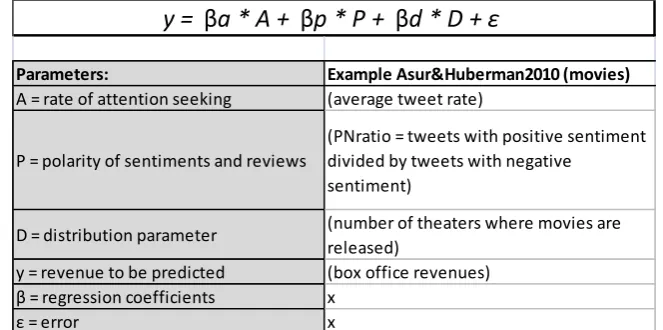
13 means that there is a strong linear relationship between the two variables. For the sentiment analysis they dealt with the classification problem of text being labelled as positive, negative or neutral. They used “thousands of workers from Amazon Mechanical Turk (https://www.mturk.com/) to assign sentiments to a large random sample of tweets”. Moreover, they assured that “each tweet was labelled by three different people”. All the samples were pre-processed by elimination of stop words, special characters and urls or user-ids. In short, they have shown that a successful predictor for box-office gross can be the average tweet-rate (per hour), 7 days prior to the movie’s release. They have also shown that sentiment analysis on a specific movie provides some improvement, but not as much as the average tweet-rate of a movie. They eventually provided a generalized model for predicting the revenue of a product using social media (see table 3.1). The adjusted R-square as a measure of the predictive power of the relationship was .973 for the variables Tweet-rate time series including the theatre count. Asur and Huberman (2010) justify this model by referring to a “collective wisdom” of users of social media, which led to the decision of investigating its power at predicting real-world outcomes. They did not refer to specific theories or models which could explain a causal relationship underlying the prediction model as Gregor (2006) proposed in her EP-theory.

Table 3.1: Prediction model designed by Asur and Huberman (2010).

In the study of Franch (2013), the independent variables were the number of YouTube views, number of mentions on Twitter, and number of mentions on Google Blogs. To extract the Twitter mentions, the Twitter application “Topsy Pro” was used. Additionally, the sentiment rating from Twitter Sentiment1 (Sentiment 140) was used as an independent variable. The dependent variable was the outcome of the British Election in 2010. The results

1_{http://twittersentiment.appspot.com/ (Sentiment 140)}

Parameters: Example Asur&Huberman2010 (movies)

A = rate of attention seeking (average tweet rate)

P = polarity of sentiments and reviews

(PNratio = tweets with positive sentiment divided by tweets with negative

sentiment)

D = distribution parameter (number of theaters where movies are released)

y = revenue to be predicted (box office revenues) β = regression coefficients x

ε = error x

14 showed that their model could predict the outcomes with an accuracy of one percent point difference with the real outcomes. They theoretically justify this model by referring to “the wisdom of the crowds” by Surowiecki (2005), “...that illustrates the predicting power of common people when their forecasts of uncertain quantities or future events are aggregated. According to this main idea, ‘boundedly rational individual(s)’ are capable of making, all together, a near-to-optimal decision, often outperforming every individual’s intelligence, meaning that the crowd, taken as an intelligent entity, is smarter than most of any human counterparts taken singularly.” They validate their model by measuring “the approval of the future Prime Minister” or “popularity of each candidate” with the before mentioned independent variables.

Goel, Hofman, Lahaie, Pennock, and Watts (2010), used web search query logs of Yahoo! Web Search to predict Box Office Revenues, the rank on a Top 100 list of a song and Video Game Sales for a specific game. In this research the number of web searches was used for predicting different outcomes, namely a rank on a top 100, box office revenue (in $) and video game sales (in units)2. Results showed that there was a strong relationship between search-based predictions and real outcomes (movies R=.94, music R=.70, and video games R=.80). They did not use the R-square as an indicator for the predictive power, however, they used the correlation coefficient to indicate a strong relationship between predicted outcomes and real outcomes. They justify the model by referring to earlier work from Asur and Huberman (2010) and Gruhl, Guha, Kumar, Novak, and Tomkins (2005), “As people increasingly turn to the Internet for news, information and research purposes, it is tempting to view online activity at any moment in time as a snapshot of the collective consciousness, reflecting the instantaneous interests, concerns and intentions of the global population.” However, the prediction studies they refer to did not comprehend any explanation of a possible causal relationship between the variables.

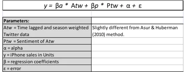
Lassen, Madsen, and Vatrapu (2014) investigated if they could predict iPhone sales based on the number of tweets with the keyword “iphone”. One of their main findings is the strength of Twitter as a social data source for predicting smartphone sales. They calculated a weighted average for the tweets every Quarter from 2010 until 2013. It is stated that the principles for monthly weighting, would follow – more or less – the same principles if monthly sales data is available. The results show that there is a strong predictive power between tweets and iPhone sales with the R-square coefficient of .95 and .96 for multiple

15 regression, with sentiment (retrieved from Topsy Pro of the same Quarter) as the second variable. The average error of the prediction model was 5-10% for the iPhone sales. The prediction model of Lassen et al. (2014) is in table 3.2. They have extended on the research of Asur and Huberman (2010), by measuring the relationship between twitter data and quarterly sales of iPhones. Therefore, they “investigate a new domain (smartphone sales), and theoretically grounding their analysis in relevant domain theory”. The underlying theory is the AIDA model, which comprehends the stages in a sales process: Awareness/Attention, Interest, Desire, and Action (Li & Leckenby, 2007). Moreover, they state that tweets are treated as a proxy for a user’s attention towards the object of analysis (the iPhone). This means that they have tried to explain the relationship between “social media data” and “real-world outcomes”.

Table 3.2: Prediction model of Lassen, Madsen & Vatrapu (2014).

3.2.2 Validity

As stated in the previous chapter, Baconian predictions come with a lot of issues, including validity. Validity refers to the extent to which an empirical measure adequately reflects the real meaning of the concept under consideration (Babbie, 2012). There are four types of validity. Face validity means that the concepts make it seem a reasonable measure for a certain variable (Babbie, 2012). For example, the frequency of attending classes, getting good grades for assignments and asking questions could be a good indicator for the level of study activity. This means it has good face validity. The face validity of the variables seems adequate for the study of Lassen et al. (2014), the amount of attention a product comprehends is represented by the amount of chatter on Twitter. Moreover, the eventual amount of purchases to be predicted is represented by factual (quarterly) sales numbers of the same products. Criterion-related validity, sometimes called predictive validity, is based on an external criterion. For example, the validity of College Board exams is shown in their ability to predict students’ success in college (Babbie, 2012). This type of validity is very strong with some of the prediction studies discussed in the previous paragraph. Researchers show that

Parameters:

Atw = Time lagged and season weighted Twitter data

Slightly different from Asur & Huberman (2010) method.

Ptw = Sentiment of Atw α = alpha

y = iPhone sales in Units β = regression coefficients ε = error

16 their model can predict future outcomes very accurate (Asur & Huberman, 2010; Goel et al., 2010; Lassen et al., 2014). However, not all of these prediction models are explained by a construct of theories, and therefore do not all comprehend causal relationships. This is called the construct validity, which is based on the logical relationships among variables. Moreover, the degree to which a measure relates to other variables as expected within the system of theoretical relationships (Babbie, 2012). “For example, studying the sources and consequences of marital satisfaction. As part of the research a measure for marital satisfaction is developed. To test its validity certain theoretical expectations of the relation of marital satisfaction to other variables will be developed. Than you might reasonably conclude that satisfied husbands and wives will less likely to cheat than dissatisfied ones. This would constitute evidence of the measure’s construct validity” (Babbie, 2012). The discrepancy between the theoretical explanations subjacent to a prediction model was elaborated in the second chapter of this thesis. An explanation for a causal relationship between the variables is not elaborated in a large proportion of previous prediction studies. Merely, they are interested in the independent variables which are linked to social media, and their potential predictive power for (future) real-world outcomes. For example, the relationship of an individual’s tweet towards an intention to buy, and therefore the eventual purchase is not validated by a theoretical construct in prediction studies. Finally, content validity refers to the degree to which a measure covers the range of meanings included within a concept. For example, when testing the degree that a person has mastered the English language, testing the vocabulary is not enough. It should comprehend all aspects, for example, grammar, spelling, adjectives and prepositions. In the field of web-search predictions, the intention to buy of an individual is merely captured by number of searches on the web. However, the intention to buy of an individual could comprehend more information search resources, such as ‘talking to a friend’ or ‘visiting stores’ to learn more about the product (Kotler, 2000).

3.3 Time lag

17 time lag is the time between (t1) attention (tweet) and (t2) action (purchase). In the study of Asur and Huberman (2010), it is debated that predictions on box office revenues are estimated one week prior to their release. Ghose and Ipeirotis (2011) studied product and sales data based on reviewer characteristics, but add ‘reviewer history’, ‘review readability’ and ‘review subjectivity’ as variables. They analyzed each review independently of the other existing reviews. They conclude that when a review is more subjective about a specific product it also shows an increase in sales for that product. Moreover, a higher ‘readability’ score is also related with higher sales. In this research they used four different time intervals (1 day, 3 days, 7 days and 14 days). The reason for this ‘time lag’ is that the researchers wanted to observe how far in time relevant and adequate predictions can be conducted and still get reasonable results. The result was that when the time lag increases, the accuracy also increases slightly. This means that reviews do not have an immediate effect particularly, but are most accurate with a time lag of 14 days. Gruhl et al. (2005) investigated if blog mentions correlated with spikes in book sales ranks on amazon.com. They concluded that when a book is mentioned more than 200 times within a specific period of time, the time lag decreases to 8.2 days. Contrary, a book that was mentioned less than 50 times, perceived a time lag of 17.2 days. However, they used a data set of 50 books and found that the time lag could differ from a couple of days to several weeks. Furthermore, the sales rank of only 10 of the 50 books were highly correlated with spikes in blog mentions. It is clear that the time lag is different for different (types of) products. Moreover, the time lag can be adjusted during the training set, so the best correlation can be found for number of tweets and number of sales for example. The function cross-correlation can be used to find the best time lag (Gruhl et al., 2005).

18 search sources) and (t2) the actual purchase of a product. The length of this time lag is dependent on two factors price and perceived risk. Research has shown that the decision time of the customer increases with the height of the price (Somervuori & Ravaja, 2013). This means the time lag could be different for expensive product types and cheap product types.

3.4 Platforms and data reliability

3.4.1 Web-search engines and microblogs

There are several platforms that can be used for predicting future outcomes. In this section, web-search- (Google and Yahoo!) and microblog (Twitter and Facebook) platforms are evaluated based on several articles. Both of these platforms should be an easy accessible data source, through API or Topsy Pro, or the pre-processed data on Google Trends and Yahoo query logs. In some of the studies an older version of Google Trends “Google Insights for Search” (GIS) was used. GIS has been shut down since 27th

of September 2012, and was merged to Google Trends. Before the shutdown of GIS, more in-depth information was publicly available3. The article of Lui, Metaxas, and Mustafaraj (2011), showed that GIS was not the best predictor for elections. There was almost no correlation between the GIS data and the actual election polls (r=.02). Contrary, the article of Vosen and Schmidt (2011) shows a different result. They investigated GIS as a predictor for private consumption. They concluded that GIS as a predictor provides better results in comparison to the generally used survey-based predictions. However, this article also dates from 2011 and used data that was available with GIS, which is not accessible anymore. Nowadays, Google Trends can provide us with a pre-processed data set of relative search volumes for a particular subject. How much of the Google Trends data differs from the GIS system is not clear. Choi and Varian (2012) studied the predictive power of Google Trends for several categories, whereas the category “Motor Vehicles and Parts” is one of the topics. Choi and Varian (2012) developed a regression model and could predict 80.8% (Adjusted R-Square: 0.808) of the variance in the dependent variable (motor vehicles and parts sales), using the independent variable (Google Trends categories of Motor Vehicles and Parts) as the predictor.

Twitter is often used as a platform to predict certain outcomes. It is used to predict election outcomes (Franch, 2013; Lui et al., 2011; Metaxas, Mustafaraj, & Gayo-Avello, 2011; Sang & Bos, 2012; Tumasjan, Sprenger, Sandner, & Welpe, 2010), disease outbreaks or influenza (Achrekar, Gandhe, Lazarus, Yu, & Liu, 2011; Culotta, 2010; Ritterman, Osborne,

19 & Klein, 2009; Signorini, Segre, & Polgreen, 2011), but also sales or revenues (Asur & Huberman, 2010; Lassen et al., 2014). Web search and Google Trends are also often used in prediction models (Bordino et al., 2012; Choi & Varian, 2012; Ettredge, Gerdes, & Karuga, 2005; Ginsberg et al., 2008; Goel et al., 2010; Guzman, 2011; Lui et al., 2011; Polgreen, Chen, Pennock, Nelson, & Weinstein, 2008; Vosen & Schmidt, 2011; Wu & Brynjolfsson, 2013). Twitter is used often, because it is an open source platform. If someone has enough knowledge of API, tweets should be easy to extract. Moreover, Twitter has proven its predictive power with high R-square values (Asur & Huberman, 2010; Lassen et al., 2014).

A platform which is less often used is Facebook. Facebook is not an open source platform. This means that messages, comments and posts are not publicly available for research (Couper, 2013). Therefore, Facebook cannot provide easy to process and accessible input data. Couper (2013) states that about one-third of the Facebook community has no demographic data available and not all users are active users. For example, it was estimated that almost 9% of the Facebook accounts is fake, duplicate, undesirable or misclassified (Couper, 2013). However, some social media monitoring sites (i.e. Social Mention, How Sociable and Brandwatch) claim they can obtain and filter messages from Facebook, for brand monitoring purposes. However, the algorithms of these monitoring tools are a black-box and we have no insight in how the messages are extracted or if it is consistent. This also acknowledged by other researchers. Chan, Pitt, and Nel (2014) just assumed that a tool like Social Mention is accurate and reliable for a measure of social media discourse. However, this is a limitation of their study. Moreover, they advocate for an independent confirmation of the trustworthiness and reliability of the data providers such as Social Mention. To gain a better understanding of the methodologies, they proposed to work directly with these services. Botha, Farshid, and Pitt (2011) support his view: “First, it would be wise to find ways of confirming the reliability and validity of data gathered by services as How Sociable. This might be done by consulting and working directly with these service providers in an effort to gain a better understanding of their methodologies and results.

3.4.2 Data reliability

20 Concluding the measurement is reliable, note that when weighing more times increases the reliability. Reliability decreases if there is only one observer, because he is probably subjective. That means that there has to be more than a single source of data to increase the reliability, and to apply the test-retest method (Babbie, 2012). However, many studies use only one source of data to base their predictions on. For example, Twitter (Asur & Huberman, 2010; Lassen et al., 2014), Google Trends (Choi & Varian, 2012), and Yahoo! Query logs (Goel et al., 2010).

Couper (2013) discussed several reliability issues of social media data. Table 3.3 shows some of the differences and similarities between social media data and survey data discussed by Couper (2013).

SOCIAL MEDIA SURVEYS

No demographic data available Demographic questions in survey

Limited type of data Type of data is only limited to type of questions

Biased (selection bias & measurement bias) Selection biases may be negligible. Measurement biases are less.

Short-term trends Long-term trends

Privacy issues Confidentially and anonymous response

possible Not all social media is easy accessible for

research purposes

Public access to the data – conditional on confidentiality restrictions and disclosure limitations.

Possibility of data manipulation Manipulation is almost impossible Large sample sizes, but not always accurate Smaller sample sizes, but more accurate

File drawer effect File drawer effect

Table 3.3: Comparison of Social Media data and Survey based data.

21 an issue that concerns both methods, social media and surveys. “The file drawer effect refers to the problem that journals are filled with 5% of the studies that show Type I errors, while the file drawers are filled with the 95% of the studies that show nonsignificant results” (Rosenthal, 1979). This means that only studies that support hypotheses that are in favour of big data are reported in journals. The Type I error refers to studies that reject the null-hypothesis, because they get significant results that the null hypothesis (e.g. against the predictive power of social media) is false. However, the null-hypothesis could actually be true. “There are many other published papers using internet searches or Twitter analyses to “predict” a variety of things... While these papers trumpet the success of the method (by showing high correlations between the organic data and benchmark measures), we do not know how many efforts to find such relationships have failed (Couper, 2013).”

3.5 Implications for this study

There are some research gaps in the field of prediction studies. Choi and Varian (2012) predicted sales of “motor vehicles and parts”. These sales numbers were based on surveys disseminated to car dealers about current sales numbers. The Google Trends’ category “motor vehicles and parts” was the independent variable. They did not investigate predicting factual sales (i.e. weekly or monthly) of specific car models with Google Trends. Moreover, they predicted the ‘present’ and encouraged that Google Trends data might predict the future, which implies that the introduction of a time lag in the model is necessary. Recent research efforts have focussed on movies (Asur & Huberman, 2010; Goel et al., 2010), video games (Goel et al., 2010), books (Gruhl et al., 2005), music (Goel et al., 2010), elections (Franch, 2013), and smartphones (Lassen et al., 2014). These studies focussed on subjects that had low risk and relatively low prices, and therefore relatively short time lags (Kotler, 2000; Somervuori & Ravaja, 2013). The question remains whether there is also great predictive power when predicting sales of products with higher risk and higher prices and thus longer time lags.

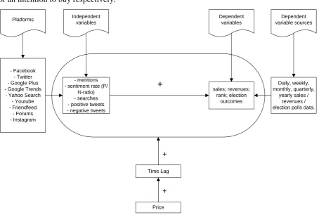
22 prediction model could enhance the initial relationship, by finding the best time lag between the number of mentions or searches and the actual purchases of products. Finally, the decision time could differ between expensive products and cheap products. Therefore, price has a positive relationship with time lag; longer time lags are related to higher prices. Based on the results from the literature review, the initial prediction model would look as follows (figure 3.1). It is constructed as a causal model, based on the assumption that a mention on social media or a search activity on Google for a specific product will comprehend a rate of attention or an intention to buy respectively.

Figure 3.1: Prediction model - mentions

- sentiment rate (P/ N-ratio) - searches - positive tweets - negative tweets

sales; revenues; rank; election

outcomes

+

Time Lag

Platforms Independent

variables

Dependent variables

Dependent variable sources

- Facebook - Twitter - Google Plus - Google Trends

- Yahoo Search - Youtube - Friendfeed

- Forums - Instagram

Daily, weekly, monthly, quarterly,

yearly sales / revenues / election polls data.

Price

+

23

4 METHODOLOGY

4.1 Research design and operationalization

24 this distinction could improve the generalizability of the prediction model for other product types. Time lag is introduced in the prediction model and could strengthen or weaken the relationship between the dependent and independent variable. Time lag is the time between a consumers search on the internet (t1) and the actual purchase of a product (t2).

Figure 4.1: Theoretical construct of consumer buying decision process towards

measurable variables.

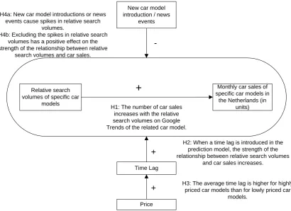
Exogenous factors like new car model introductions or news events could have a negative effect on the relationship between search volumes and car sales. This is based on the assumption that when a new car model is announced, this car model will get a large amount of attention. This spike in search volumes could exists of a large proportion of consumers that have no intention to buy. This results in a discrepancy between relative number of searches and the actual sales, which will occur several months later when the car is actually available for consumers. Simplifying the previous model and introducing the time lag, which could be explained by price according to the theory of decision time of consumers (Somervuori & Ravaja, 2013), and adding the new car model introduction (news) variable gives the following research design (figure 4.2), with the corresponding hypotheses. In the next paragraphs the data collection and methods of analysis for the hypotheses will be elaborated

Stage 1: Problem recognition

Stage 2: Information

search

Stage 3: Evaluation of

alternatives

Stage 4: Purchase

decision

Stage 5: Post-purchase behaviour

Search on Google

CONSUMER BUYING DECISION PROCESS BY KOTLER (2000)

Time lag Purchase

Relative search

volumes Time lag

25

Figure 4.2: Research model: prediction model for car sales and hypotheses.

4.2 Data collection

The sales data of cars are derived from the website of BOVAG4. A list of the selected car models is in appendix B. There are 68 different car models (N=68) selected based on the number of sales. Note that not all car models are sold throughout all seven years, some models were launched later and some were removed from the product range earlier. The data from the website is processed in a .PDF file on the website of BOVAG. This file shows the number of sales of specific car models on a monthly basis for the Netherlands. This data is entered in an SPSS database to analyze the data. This has been done manually for some specific months, because the free converting tool for scanned images within a .PDF file limits the converting of .PDF files to one page only. The sales data extracted from BOVAG runs from January 2008 to December 2014 (7 years). The sample size of seven years is based on the assumption that the larger the sample size, the less the variability in the collected data will be when used for forecasting purposes (Hyndman & Kostenko, 2007). Hyndman and Kostenko (2007) stated that “the sample size has to be as large as possible” to exile as much of the variability in the data as possible, for forecasting purposes. Real data often contain a lot of random variation, and sample size requirements increase accordingly (Hyndman &

4_{http://www.bovag.nl/over-bovag/cijfers/verkoopcijfers-auto} Relative search

volumes of specific car models

Monthly car sales of specific car models in

the Netherlands (in units)

+

Time Lag

Price +

+

H1: The number of car sales increases with the relative search volumes on Google Trends of the related car model.

H2: When a time lag is introduced in the prediction model, the strength of the relationship between relative search volumes

and car sales increases.

H3: The average time lag is higher for highly priced car models than for lowly priced car

models. New car model

introduction / news events

-H4a: New car model introductions or news

events cause spikes in relative search volumes.

H4b: Excluding the spikes in relative search volumes has a positive effect on the strength of the relationship between relative

26 Kostenko, 2007). The sales data is for the Netherlands only, which means that the trends data has to be demarcated for Dutch searches only.

The trends data could be collected through the ‘export to .CSV’ option, which can be opened in MS Excel and should provide the correct data. However, when selecting the specific time periods (i.e. January 2008 to December 2014) the data is still exported per week number instead of months. Consequently, some week numbers would cover two different months. Moreover, the online graph of Google Trends does show the relative search volumes per month. Therefore, all figures were entered in the database manually, by sliding over the graph and entering the right numbers in SPSS. In order to preserve the validity and reliability of the independent variables, the keywords used in Google Trends are the same as the car model names in the BOVAG sales figures (e.g. “Volkswagen Golf”, “Peugeot 107”). The quotation marks ensure that the car model names are not taken out of context (i.e. “Golf” could refer to other synonyms like the sport). Moreover, not every individual searching for a Volkswagen starts with the entire word, so acronyms like “VW Golf” are also taken into account. In Google Trends specific periods of time can be selected and therefore makes a good and flexible independent variable. To ensure the content validity of the keywords representing the car models that are selected, the option “Automobiles and Vehicles” is selected. By doing this, Google Trends excluded other contexts of the specific keywords. For example, when selecting “Citroën C4 Picasso” it excludes the interpretations of the painter Picasso in the search results. Another demarcation is location based. Only searches that were located in the Netherlands are demarcated by Google Trends. The average car prices are derived from the Top Gear5 (Dutch version) website and are in Euro (€). The new model announcement dates and news items are derived from Autoweek.nl, Google News, and Topgear.nl.

27

4.3 Methods of analysis

To analyze the first hypothesis, the monthly average for the trends and the sales of each car model is calculated. Subsequently, the relationship between TRENDS_average and SALES_average is tested in SPSS for a correlation (Analyze > Regression > Linear). The significance (p-value) of this relationship is key for the decision if the null hypothesis (no relationship) will be rejected or not. A confidence interval of 95% is applied. If the p-value is smaller than .05, the null hypothesis is rejected, when the p-value is larger than .05, the null hypothesis (no relationship) is accepted. The correlation coefficient ‘R’ is a measure of showing the direction and strength of the linear relationship between two variables. Moreover, the predictive power is represented by the R-square. This aligns with the methods used by Asur and Huberman (2010) and Choi and Varian (2012), where the R-square reflects the predictive power of the independent variable within the regression model.

28 (Analyze > Forecast > Cross-Correlation). Thereafter, the time lag is applied, a linear regression analysis is conducted, and the results are also listed in the table. Finally, the changes in the R-square indicate whether the predictive power has changed, and what the best time lag should be. If there are significant improvements in strength and predictive power, the null hypothesis (no improvement) is rejected and the alternative hypothesis (improvement) is accepted. The steps are outlined in table 4.1.

Step 1 Linear regression of original relationship between trends and sales of a specific car. Report results in table.

Step 2 Cross-correlation on the trends and sales data to calculate the best time lag. Apply the time lag on the sales data (i.e. instead of matching the trends data of jan-2005 to the sales data of jan-2005, match jan-2005 to apr-2005 respectively, lag = 3).

Step 3 Linear regression of the relationship between trends and sales of a specific car, with the applied time lag. Report results in table.

Step 4 Calculate improvements in R, R-square and significance. Report results in table.

Table 4.1: Steps for introducing time lag into the prediction model.

For the third hypothesis, the best time lag for each car model has to be calculated in SPSS. This is conducted by using the cross-correlation option (Analyze > Forecast > Cross-Correlation), which is also used in the previous hypothesis. After finding the best time lag for each car model, the new variable ‘best_time_lag’ is created. The car prices are divided into two categories, lowly priced cars (N=37) and highly priced cars (N=31), with the values of ≤24.999 and 25.000< respectively. Subsequently, an independent t-test is conducted for the mean time lags of both categories. The results of this test indicate if there is a difference between the mean time lags of lowly- and highly priced cars. The same alpha level is applied, if the p-value is below .05 the null hypothesis (no difference in lag) will be rejected, and the alternative hypothesis (difference in lag) will be accepted.

29 spike(s) are excluded. Additionally, a time lag will be introduced into the new model and the linear regression results will also be listed in the table. The changes in the R-square indicate whether the predictive power has changed. If there are significant improvements in strength and predictive power, the null hypothesis (no improvement) is rejected and the alternative hypothesis (improvement) is accepted. The six-step method is outlined in table 4.2.

Step 1 Linear regression of original relationship between trends and sales of a specific car. Report results in table.

Step 2 Spike(s) in the trends data will be identified for the car model. This is done by plotting a graph of the trends data and locating the moment of the lowest value prior to the spike and associating this spike with the corresponding news or new car model introduction for that date.

Step 3 The cases (months) during the spikes are excluded from the data set.

Step 4 Linear regression of the relationship between trends and sales of a specific car, with spike(s) excluded. Report results in table.

Step 5 Introduce calculated time lag into the prediction model. Linear regression of the relationship between trends and sales. Report results in table.

Step 6 Calculate improvements in R, R-square and significance for exclusion of spikes and introduction of time lag. Report results in table.

30

5 ANALYSIS & RESULTS

For the first hypothesis the average of trends and sales per car model for all years are calculated. A linear regression analysis is conducted for these two variables. Table 5.1 shows the correlation coefficient. In this case we can see R=.345 indicating a positive relationship between trends and sales, significant at p<0.01. However, the relationship appears to be weak. Furthermore, how would this relationship fit into a prediction model? Table 5.1 presents that the R-square is.119, which means that approximately 12 percent of the variance in the dependent variable is explained by the independent variable. This is a low R-square coefficient compared to other studies (i.e. Asur and Huberman (2010), Adjusted R-square=.94 and Choi and Varian (2012), Adjusted R-square=.808). However, the adjusted R-square is only used when more (i.e. moderating) variables or predictors are introduced into the regression model, which is not the case in this study.

Table 5.1: Model summary of linear regression with trends as independent variable.

31 regression analysis results of the BMW 5-serie data without a time lag are in table 5.2. These results are also listed in table 5.4.

Table 5.2: Model summary of linear regression for the BMW 5-series without time lag.

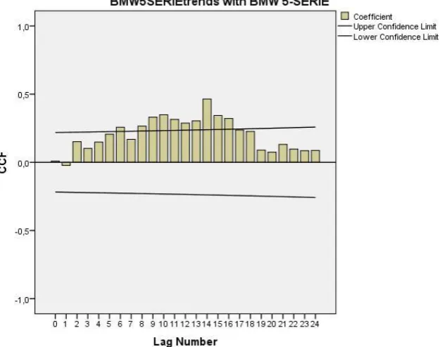
When these results are noted, the next step is to conduct a cross correlation for the trends and sales data. The results are in histogram figure 5.1. The cross-correlation shows that there could be a stronger relationship at a time lag of 14 months. In figure 5.1 we can see that the correlation coefficient corresponding to the lag number 14 is also significant at a confidence level of 95%.

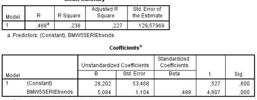
32 The next step is to conduct a linear regression analysis with the 14 month time lag applied. For the BMW 5-serie the results are in table 5.3. It shows that the correlation coefficient is now R=.488, the R-square =.238 and significant at p<.001.

Table 5.3: Model summary of linear regression for the BMW 5-serie with 14 months time lag.

CAR MODELS LINEAR REGRESSION

RESULTS (no time lag)

LINEAR REGRESSION RESULTS (after identifying the

best time lag)

Improvements

R R² Sig. R R² Sig. Lag R²

Audi A6 .049 .002 .657 .237 .056 .048 14 +5.4% BMW 5-serie .008 .000 .941 .488 .238 .000 14 +23.0% Citroen C3 .413 .171 .000 .553 .305 .000 12 +13.4% Citroen C5 .481 .231 .000 .826 .682 .000 6 +45.1% Ford Focus .349 .122 .001 .349 .122 .001 0 0 Hyundai i10 .006 .000 .957 .030 .001 .790 3 +0.1% Hyundai ix35 .574 .330 .000 .726 .527 .000 3 +19.7% KIA Sportage .653 .427 .000 .653 .427 .000 0 0 Mercedes B Class .193 .037 .078 .501 .251 .000 6 +21.4% Mercedes E Class .128 .016 .246 .322 .104 .004 4 +8.8% Nissan Juke .365 .133 .008 .718 .515 .000 3 +38.2% Opel Corsa .010 .000 .930 .367 .135 .001 10 +13.5% Peugeot 107 .609 .371 .000 .609 .371 .000 0 0 Seat Leon .315 .099 .004 .648 .420 .000 11 +32.1% Toyota Auris .608 .370 .000 .684 .467 .000 5 +9.7% Volkswagen Jetta .153 .024 .163 .659 .435 .000 6 +41.1% Volkswagen UP! .023 .001 .885 .604 .365 .000 6 +36.4%

Table 5.4: Differences before and after introducing time lag in the prediction model.

33 fourteen out of the seventeen (82%) car models have a time lag. When this time lag is applied the predictive power increases for these relationships between relative search volumes and car sales. This indicates that the null hypothesis when time lag is introduced in the model, the predictive power of the relationship between relative search volume (trends) and car sales (sales) show no improvements, is rejected. Therefore, the alternative hypothesis of introducing a time lag in the model, the predictive power of the relationship between trends and sales improves, is accepted. The high significance level and level of predictive power of the Hyundai i10 cannot be explained, since the same steps are repeated for each car model.

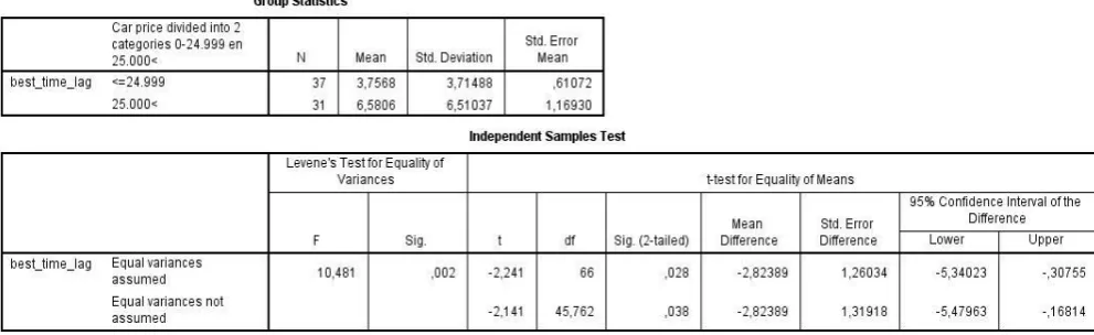
For the third hypothesis, it is expected that the average time lag is higher for highly priced car models than for lowly priced car models. Therefore, for each car model the best time lag was computed. This is done by using the cross-correlation function in SPSS (Analyze > Forecast > Cross-Correlation). This same function was used in the previous hypothesis, to locate the best time lag. Subsequently, a list of best time lags for each car model was created, and a list with all the car prices corresponding to the same car models. The car models are divided in two categories, lowly priced cars and highly priced cars, with the values ≤24.999 and 25.000< respectively. Finally, an independent t-test for the means of the time lags of both categories is executed. The results of the t-test are in table 5.5.

Table 5.5: Independent t-test for the means of the time lags, sorted by price category.

34 cars, where highly priced cars have a larger average time lag. This means that the hypothesis that the time lag is higher for highly priced cars than for lowly priced cars, is supported.

Finally, the relationship could be influenced by the introduction of new car models or other news which causes spikes in search volumes within the time span of seven years the data is collected. Therefore, an additional analysis will be conducted, following six steps. First, a linear regression analysis of the seventeen car models used in the previous analysis will be conducted. Subsequently, the spike(s) in the trends data will be identified for the car models. Thirdly, the observations during these spikes will be excluded. A linear regression analysis will be carried out for the car models, where the observations during the spike(s) are excluded. For example, the Peugeot 107, shows a few spikes in the trends data (see fig. 5.2). The results of the linear regression analysis for trends and sales for the Peugeot 107 are in table 5.6. The R=.609 and R-square =.371, significant at p<.001. This indicates a moderate relationship between trends and sales, and very significant.

Table 5.6: Linear regression analysis for the Peugeot 107 (Jan.2008 – Dec. 2014).

35 The next step is to identify the spikes in the trends data. There was no introduction of a new model before the spikes occur. However, for the identification of the first spike “Peugeot 107” was entered into Google. Subsequently, the results were filtered on “news” for the “Netherlands” and for the period “October 2009 – April 2010” and “October 2010 – April 2011”. In this graph the events before the actual spikes occur are marked with an X-axis reference line:

- Jan 2010: announcement of the recall action for Peugeot 107 and Citroën C1 in the news (Telegraaf).6

- Dec 2010: start of the recall action for Peugeot 107 in the news on Autoweek, NRC and NOS.7

The cause of the third spike (August 2011) could not be identified using this method. The next step is to exclude the months of the spikes. This can be done in SPSS by selecting individual cases (a case represents one month). Subsequently, a linear regression analysis is conducted for the period January 2012 – December 2014, because the spike effect has worn off approximately around January 2012.

Table 5.7: Linear regression analysis trends and sales for the Peugeot 107 (January 2012 – December 2014).

The results of the linear regression analysis (table 5.7) show that R=.887 and R-square =.786, significant at p<0.001. There is an improvement of 41.5% in the amount of variance that can be explained in the dependent variable after excluding the spikes in the trends data for the Peugeot 107. A table (5.8) is conducted for the results performing this six-step analysis for the

6

http://www.telegraaf.nl/autovisie/autovisie_nieuws/20400729/__Ook_terugroepactie_voor_Peugeot_107_en_Ci troen_C1__.html

7

http://nos.nl/artikel/206419-terugroepactie-het-woord-van-de-autobranche.html;

36 other sixteen car models before and after spike exclusion. Subsequently, the time lag is applied, and the linear regression results are also reported in table 5.8.

CAR MODEL (including the event before the spike)

Linear regression results spikes

included

Linear regression results spikes

excluded

Linear regression results spikes excluded and time

lag applied

R R² Sig. R R² Sig. R R² Sig. Lag

Audi A6 (Pro Line S model Jun. 2010) .049 .002 .657 .086 .007 .545 .559 .312 .000 14 BMW 5-series (new model Nov. 2009) .008 .000 .941 .336 .113 .013 n/a n/a n/a 0 Citroen C3 (new model Jun. 2009) .413 .171 .000 .467 .218 .000 n/a n/a n/a 0 Citroen C5 (new model Oct. 2007) .481 .231 .000 .636 .404 .000 n/a n/a n/a 0 Ford Focus (new model Feb. 2011) .349 .122 .001 .649 .421 .000 n/a n/a n/a 0 Hyundai i10 (new model Aug. 2013) .006 .000 .957 .320 .102 .010 n/a n/a n/a 0 Hyundai ix35 (new model Sep. 2009) .574 .330 .000 .698 .487 .000 n/a n/a n/a 0 KIA Sportage (new model Apr. 2010) .653 .427 .000 .599 .359 .000 n/a n/a n/a 0 Mercedes B (new model Aug. 2011) .193 .037 .078 .266 .071 .085 .657 .432 .000 2 Mercedes E (new models late 2009) .128 .016 .246 .169 .029 .155 .361 .130 .002 4 Nissan Juke (new model Feb. 2010) .365 .133 .008 .515 .265 .000 .561 .315 .000 3 Opel Corsa (new model Nov. 2009) .010 .000 .930 .238 .057 .085 .493 .243 .000 4 Peugeot 107 (recall in Jan./Dec. 2010) .609 .371 .000 .887 .786 .000 n/a n/a n/a 0 Seat Leon (new models May 2009) .315 .099 .004 .365 .133 .003 .746 .557 .000 11 Toyota Auris (new model Sep. 2009) .608 .370 .000 .458 .210 .001 .620 .384 .000 6 Volkswagen Jetta (new hybrid Oct. 2012) .153 .024 .163 .163 .027 .221 .499 .249 .000 6 Volkswagen UP! (new model Jul. 2011) .023 .001 .885 .428 .183 .037 .536 .288 .008 1

Table 5.8: Differences before and after excluding spikes in the trends data for six car models.

37

CAR MODEL IMPROVEMENT

IN R-SQUARE AFTER EXCLUDING SPIKES

IMPROVEMENT IN R-SQUARE AFTER EXCLUDING SPIKES AND APPLYING TIME LAG

Audi A6 +0.5% +31.0%

BMW 5-serie +11.3% n/a (time lag 0)

Citroen C3 +4.7% n/a (time lag 0)

Citroen C5 +17.3% n/a (time lag 0)

Ford Focus +29.9% n/a (time lag 0)

Hyundai i10 +10.2% n/a (time lag 0)

Hyundai ix35 +15.7% n/a (time lag 0)

KIA Sportage -6.8% n/a (time lag 0)

Mercedes B Class +3.4% +39.5% Mercedes E Class +1.3% +11.4% Nissan Juke +13.2% +18.2% Opel Corsa +5.7% +24.3% Peugeot 107 +41.5% n/a (time lag 0)

Seat Leon +3.4% +45.8% Toyota Auris -16.0% +1.4% Volkswagen Jetta +0.3% +22.5% Volkswagen UP! +18.2% +28.7%

Table 5.9: Improvements in R-square of the relationship between trends and sales.

38

6 CONCLUSION & DISCUSSION

6.1 Key findings

The intention of this thesis was to investigate the reliability and validity of web-search based predictions. Five hypotheses were tested for testing the relationship between search volumes and sales. The results of the analysis were as follows. The first hypothesis “the number of car sales increases with the relative search volumes on Google Trends of the related car model” is supported. However, the relationship is weak (R=.345). Approximately 12% of the variance in the car sales could be predicted by the relative search volumes. The second hypothesis “when a time lag is introduced in the prediction model, the strength of the relationship between relative search volumes and car sales increases”, is supported. Moreover, for approximately 82% of the analyzed car models the predictive power increased after introducing the time lag in the prediction model. The third hypothesis, “the average time lag is higher for highly priced car models than for lowly priced car models” is supported. Highly priced car models have an average time lag of 6.6 months and lowly priced car models have an average time lag of 3.8 months. The final two hypotheses, “new car model introductions or news events cause spikes in relative search volumes” and “excluding the spikes from relative search volumes has a positive effect on the strength of the relationship between relative search volumes and car sales” are both supported. Moreover, the analysis showed that new car model introduction caused spikes in relative search volumes, and not followed by spikes in sales afterwards. When the spikes were excluded, the strength of the relationship of 88% for the analyzed car models increased. Introducing the time lag after exclusion of spikes, showed that the strength increased further for 53% of the selected car models. For the remaining 47% of the car models, the strength of the relationship did not increase and there was no time lag.

40

6.2 Discussion

This thesis Choi and Varian

(2012)

Vosen and Schmidt (2011)

Methods Linear regression analysis. Auto Regressive (1) model.

Auto Regressive model.

Platforms Google Trends Google Trends Google Trends

Independent variables

relative number of searches for 68 car models in the Netherlands.

relative number of searches for different categories in Google Trends.

relative number of searches for 56 different categories of private consumption. And survey-based indicators.

Dependent variables

Factual sales in the Netherlands for 68 car models.

Sales in Motor vehicles and Parts based on surveys sent to dealers worldwide.

Personal consumption expenditures (PCE) of 18 categories. Corresponding to the 56 Google Trends categories which are distributed to the 18 categories of PCE.

Timelag included?

Yes, up to 24 months.

For each car model the best time lag was computed within the 24 month-frame, and tested if taking time lag into account improved the predictive power.

The 12 month lag is only used for estimating the baseline. It is not tested if time lag has an effect on the predictive power.

Yes, 1 month.

Differences in nowcasting (h=0; no time lag) and forecasting (h=1; 1 month time lag) are compared on predictive power.

Predictive power indicator

R-square.

(improvements in R-square)

R-square and Mean Absolute Error (MAE). (improvements in MAE)

Incremental Adjusted R-square changes.

Root Mean Squared Forecast Errors (RMSFEs).

RESULTS -Takingtime lag into account increases the predictive power - Excluding spikes caused by certain events in search volume data increases the predictive power. - The magnitude of the time lag increases with price. And differs per car model.

-Google trends predicts the present with 80.8% predictive power (R-square =.808).

-Google Trends prediction models, have better results in forecasting consumption than survey-based predictions.

Assessing the reliability and validity of predictions based on relative search volumes.

Claim they are predicting the present instead of the future.

Claim predicting the future and the present of private consumption.

Table 6.1: Comparison of this study with similar studies (Choi & Varian, 2012; Vosen & Schmidt,

2011).