University of Warwick institutional repository
This paper is made available online in accordance with publisher policies. Please scroll down to view the document itself. Please refer to the repository record for this item and our policy information available from the repository home page for further information.
To see the final version of this paper please visit the publisher’s website. Access to the published version may require a subscription.
Author(s): Chen, Yunfei, Beaulieu, Norman C.
Article Title: Maximum likelihood receivers for space-time coded MIMO systems with gaussian estimation errors
Year of publication: 2009 Link to published version:
Maximum Likelihood Receivers for
Space-Time Coded MIMO Systems with
Gaussian Estimation Errors
Yunfei Chen , Member, IEEE, Norman C. Beaulieu, Fellow, IEEE
Corresponding Address:
Yunfei Chen
School of Engineering
University of Warwick, Coventry, U.K. CV4 7AL
Tel: +44 (0)24 765 23105
e-mail:
[email protected]
Yunfei Chen is with the School of Engineering, University of Warwick, Coventry, U.K. CV4 7AL (e-mail:
Norman C. Beaulieu is with the Department of Electrical & Computer Engineering, University of Alberta, Edmonton, Alberta,
Abstract
Maximum likelihood (ML) receivers for space-time coded multiple-input multiple-output (MIMO)
systems with Gaussian channel estimation errors are proposed. Two different cases are considered.
In the first case, the conditional probablity density function (PDF) of the channel estimate is assumed
Gaussian and known. In the second case, the joint PDF of the channel estimate and the true channel
gain is assumed Gaussian and known. In addition to ML signal detection for space-time coded MIMO
with ML and minimum mean squared error channel estimation, ML signal detection without channel
estimation is also studied. Two suboptimal structures are derived. The Alamouti space-time codes are
used to examine the performances of the new receivers. Simulation results show that the new receivers
can reduce the gap between the conventional receiver with channel estimation errors and the receiver
with perfect channel knowledge at least by half in some cases.
Index Terms
channel estimation, imperfect, maximum likelihood, MIMO.
I. INTRODUCTION
Multiple-input multiple-output (MIMO) techniques have been well recognized as effective
methods for increasing the reliability and the data rate of a wireless communication system
[1]- [4]. The results in [1]- [4] are based on the assumption of perfect channel knowledge. In
practice, however, perfect channel knowledge is never available. Instead, one has to estimate the
channel. When the channel is estimated, estimation errors will occur. These estimation errors
cause performance degradations. Therefore, the system performances reported in [1]- [4] are
only upper limits, and the exact performances of MIMO systems with channel estimation errors
are yet to be determined. Inspired by this, many researchers have examined the effect of channel
estimation errors on the performances of MIMO systems. For example, in [5]- [9], the effect of
channel estimation errors on the capacities of MIMO systems has been evaluated. These results
give the maximum achievable transmission rates or the multiplexing gains of MIMO systems
when the channel knowledge is not perfectly known. In [10]- [14], the authors analyzed the
gain due to imperfect channel estimation can be determined from these results.
In addition to the analyses of the channel capacities and the error rates of MIMO systems with
channel estimation errors in [5]- [14], several researchers have also studied ways of improving
the performances of MIMO systems when channel estimation errors occur. For example, in
[15]- [18], several methods were proposed to improve the performances of MIMO systems by
optimizing the pilot powers and the pilot positions. In [19], by assuming a Gaussian channel
estimation error and using the correlation between the channel estimate and the true channel
gain, the authors derived the optimum maximum likelihood receiver for space-time coded
sig-nals in the presence of channel estimation errors. This receiver design is valid for orthogonal
space-time codes. In [20], the authors derived the optimum maximum likelihood receiver for
any space-time code, which can be regarded as a generalization of the receiver in [19]. The
results in [19] and [20] suggest that one can improve the performances of MIMO systems by
using additional knowledge of the joint statistics of the channel estimate and the true channel
gain. This conclusion agrees with those made in [21], where a single-input and multiple-output
diversity system was considered. Motivated by this observation, in this paper we extend the
results in [20] to two more general cases by using methods similar to those in [21].
Specifically, in this paper, we derive the maximum likelihood (ML) receivers for space-time
coded MIMO systems when channel estimation error is Gaussian and particular additional
knowledge of statistics of the channel estimate and/or the true channel gain is available. The
assumption of Gaussian estimation error is justfied by the fact that many channel estimation
er-rors are determined by Gaussian noise in the estimation, as can be seen from [20] as well as (6)
and (8) in the next section. It is also justified by the fact that many well-designed estimators are
asymptotically Gaussian when the sample size is large [22]. We assume a block-fading channel,
where the length of a data packet is chosen to be smaller than the channel coherence time, to
simplify the receiver design, similar to [19] and [20]. Two different cases are discussed. In
condi-tioned on the true value of the channel gain, is assumed Gaussian and known. The conditional
Gaussian PDF of the channel estimate can be obtained by analyzing or simulating the mean and
the variance of the channel estimates. In the second case, in addition to the conditional PDF of
the channel estimate, conditioned on the true channel gain, the PDF of the true channel gain is
also assumed Gaussian and known, which is the case when the MIMO channels are Rayleigh
or Ricean faded. Therefore, we assume a joint Gaussian PDF for the channel estimate and the
true channel gain. We derive the general structures of the ML receivers in both cases. Based on
these general structures, we then study two special cases when the ML channel estimator and the
minimum mean squared error (MMSE) channel estimator are used. These receivers presumably
work in two steps: a first step of using the pilot symbols for channel estimation and a second
step of using the data symbols and the channel estimates for signal detection. To make this study
fully comprehensive, we also propose ML receivers without channel estimation, where the pilot
symbols are used directly in the signal detection. Finally, we present two suboptimal receivers
with simplified structures and compare their performances with the conventional receivers by
simulation.
The remainder of this paper is organized as follows. In Section II, the system model is
intro-duced. In Section III, the ML receivers for the first case are presented where only the conditional
PDF of the channel estimate is known. Section IV discusses the ML receivers in the second case
where the joint PDF of the channel estimate and the true channel gain is known. Numerical
results are shown in Section V.
II. SYSTEM MODEL
A. Channel Model
Consider a MIMO system withttransmitter antennas andrreceiver antennas. The transmitter
sends data packets withN data symbols and M pilot symbols to the receiver. For simplicity,
we assume that the firstN symbols in the data packet are data symbols and the following M
gain remains approximately the same during the transmission of the whole data packet, similar
to [19] and [20]. The received data symbols can be expressed as
Y=CX+Z (1)
whereYis ar×N matrix representing the received data symbols,Y = [Y1 Y2 · · · Yr]T with the i-th rowYi = [Yi1 Yi2 · · · YiN], i = 1,2,· · · , r, T denotes the transpose oper-ation, Cis ar×t matrix representing the MIMO channel gains,C = [C1 C2 · · · Cr]T with thei-th rowCi = [Ci1 Ci2 · · · Cit], i = 1,2,· · · , r, Xis at×N matrix represent-ing the transmitted space-time coded signals,X = [X1 X2 · · · XN]with thej-th column Xj = [X1j X2j · · · Xtj]T,j = 1,2,· · · , N, andZis ar×Nmatrix representing the noise, Z= [Z1 Z2 · · · Zr]T with thei-th rowZi = [Zi1 Zi2 · · · ZiN],i= 1,2,· · ·, r.
DenoteC˜ = [C1 C2 · · · Cr] as the 1×rt channel gain vector. Assume a separable Kronecker correlation model. In a Ricean fading channel, the elements of C˜ are assumed to
be circularly symmetric complex Gaussian random variables with mean E{Ci} = mi, i =
1,2,· · · , r, and rt×rtcovariance matrix 2α2R⊗T, where2α2 is the mean fading power of the scattering component,Rrepresents ther×rcovariance matrix of the receiver antennas, T represents thet×tcovariance matrix of the transmitter antennas, and⊗represents the Kronecker product. In [23] and [24], a Bessel model and an exponential model have been proposed for
the antenna correlations, respectively. We assume equi-spaced antennas and use the Bessel
model in this paper. Therefore, the(i, j)-th element ofR satisfiesR(i, j) = J0 2πdλr|i−j|
, i, j = 1,2,· · · , r, and the (i, j)-th element of T satisfies T(i, j) = J0 2πdλt|i−j|
variables each with mean zero and variance2σ2. Further,Cis independent ofZ.
Using (1), the likelihood function can be expressed as
f(Y|C,X) = 1 (2πσ2)rNe
− 1 2σ2
Pr
i=1(Yi−CiX)(Yi−CiX)H
(2)
whereH represents the Hermitian transpose. When the channel gainCis perfectly known, one
has the ML receiver as
ˆ
X= arg min
X {tr (Y−CX)(Y−CX)
H
} (3)
where tr(·) denotes the trace of a matrix. We denote (3) as the genie receiver. In practice, it is impossible to know the channel gain matrix C perfectly. Instead, one has to use the pilot
symbols in the data packet to estimate it.
B. Channel Estimation
The received signals of the pilot symbols can be written as
Q=CP+W (4)
where Q is a r × M matrix representing the received signals of the pilot symbols, Q = [Q1 Q2 · · · Qr]T with the i-th row Qi = [Qi1 Qi2 · · · QiM], i = 1,2,· · · , r, P is at×M matrix representing the transmitted pilot symbols,P = [P1 P2 · · · PM]with thej-th columnPj = [P1j P2j · · · Ptj]T,j = 1,2,· · · , M, andWis ar×M matrix rep-resenting the noise corrupting the pilot symbols, W = [W1 W2 · · · Wr]T with the i-th row Wi = [Wi1 Wi2 · · · WiM], i = 1,2,· · · , r. Similar to [20], we assume that M ≥ t, Pis known,(PPH)−1 exists andPPH is real.
Using (4), the ML channel estimator forCcan be derived by finding ther×tmatrixCˆ that minimizes||Q−CP||2, where || · ||2 is the sum of the squares of all elements in the matrix. It was derived in [20] that the ML channel estimator is given by
ˆ
whereCˆ is ther×tmatrix representing the channel gain estimates,Cˆ = [ ˆC1 Cˆ2 · · · Cˆr]T with the i-th row Cˆi = [ ˆCi1 Cˆi2 · · · Cˆit], i = 1,2,· · · , r. For later use, denote C˜ˆ =
[ ˆC1 Cˆ2 · · · Cˆr]as the channel estimate vector. Using (4) in (5), one has
ˆ
C=C+WPH(PPH)−1. (6)
Therefore, the ML channel estimatorCˆ gives an unbiased estimate ofCwith a Gaussian
esti-mation error ofWPH(PPH)−1.
When the covariance matrix of the channel gains and the mean channel matrix are known,
the MMSE channel estimator for C can also be derived by finding the M ×t matrix Fˆ that minimizesE{||QF−C||2}. After some manipulations, the MMSE channel estimator can be derived as
ˆ
C=QFˆ (7)
whereFˆ = (PHTP+σ2
α2IM×M+P
HmH
m
2α2r P)−
1PH[T+mH m
2α2r]andIM×M is theM×M identity
matrix. Compare (7) with [20, eq. (12)], one sees that [20, eq. (12)] is a special case of (7) when
T=It×tandm=0. Further, using (4) in (7), one has
ˆ
C=CPFˆ +WFˆ (8)
which gives a biased estimate ofC. This bias can be removed by multiplying both sides of (8)
with (PFˆ)−1 from the right, when (PFˆ)−1 exists. Note that the MMSE channel estimator in
(7) can only be used when the covariance matrix of the transmitter antennas T and the mean
channel matrixmare known.
Using these channel estimates, the receiver decision rule
ˆ
X= arg min
X {tr
(Y−CXˆ )(Y−CXˆ )H} (9)
has been widely used in current systems. In this paper, we will design new receivers that improve
upon the performance of (9). These new receivers can be obtained by processing the channel
of the true channel gain is needed. They can also be obtained by using additional knowledge of
the statistics of the true channel gain, similar to [20]. However, [20] only considered the case
when the MIMO channels are independent and identically distributed. Here, we obain results
for the case of correlated MIMO channels.
III. CONDITIONALPDFOF CHANNELESTIMATE
In the first case, no extra knowledge of the true channel gain is available. One only knows
the conditional Gaussian PDF of the channel estimate, conditioned on the true channel gain.
This knowledge is available for many receivers by analysis or simulation of the estimator
per-formance. Therefore, one has
f( ˆC|C) = 1 (2π)rt|∆
1| e−12
Pr
i1 =1
Pr
i2 =1( ˆCi1−Ci1A(i1)−B(i1))∆− 1
1 (i1,i2)( ˆCi2−Ci2A(i2)−B(i2))H
(10)
where∆1is thert×rtcovariance matrix ofRe{C˜ˆ}orIm{C˜ˆ},Re{·}andIm{·}give the real and imaginary part of a complex number, respectively,∆−11(i1, i2)is the(i1, i2)-th submatrix of
∆−11 obtained by evenly partitioning∆−11 into a r×r block matrix, andE{Cˆi} = CiA(i)− B(i). Using (10) and (2), it can be shown that
f(Y,Cˆ|X) =
Z
· · ·
Z
f(Y|C,X)f( ˆC|C)dC
= D1
|∆˜1| e12u ˜∆
−1 1 u
H
(11)
whereR · · ·R
represents art-dimensional integral,dC= dC11· · ·dCrt,D1 is a constant inde-pendent ofX,∆˜1is art×rtmatrix which can be partitioned into ar×rblock matrix with the
(i1, i2)-th submatrix∆˜1(i1, i2) =A(i1)∆−11(i1, i2)AH(i2) + XX
H
σ2 ,| · |denotes the determinant
of a matrix, u = [u1 u2 · · · ur]andui = YiX
H
σ2 +
Pr
i1=1( ˆCi1 −B(i1))∆
−1
1 (i1, i)AH(i)
withi= 1,2,· · · , r. The optimum ML receiver in this case can be derived from (11) as
ˆ
X= arg min
X {ln|
˜ ∆1| −
1 2u ˜∆
−1
Comparing (12) with (9), one sees that there is an additional bias term of ln|∆˜1| in the new receiver. In general, (12) is not equivalent to (9). The receiver in (12) applies to all fading
channel models, including Ricean, Nakagami-m and Laplacian channels, as no knowledge of
the statistics of the true channel gain is assumed in the derivation. It also applies to any channel
estimators satisfying (10).
A special case occurs when the ML channel estimator in (5) is used. In this case, one further
has
ˆ
X = arg min
X
rln|PPH +XXH|
−
tr(YXH + ˆCPPH)[PPH +XXH]−1(YXH + ˆCPPH)H
2σ2
(13)
since from (6), one hasA(i) = It×t, B(i) = 0and∆1 =Ir×r⊗[σ2(PPH)−1]. Note that the optimum receiver in (13) is equivalent to the conventional receiver in (9) whenXXH is constant
for allX. Note also that the MMSE channel estimator cannot be used here, as no knowledge of
the covariance matrixTand the mean channel matrixmis available in this case.
Observe that both the receiver in (9) and the receiver in (12) involve a two-step procedure.
In the first step, channel estimation is performed by using Q to obtain an estimate Cˆ. In the
second step, signal detection is performed by using Y and Cˆ. The only difference is in the
second step whereYandCˆ are processed using (9) in the conventional receiver, while they are
processed using (12) in the optimum receiver. As a further study, it is also of interest to examine
the detection ofXwithout using channel estimation [20]. From (4), the likelihood function of
the pilot symbols can be expressed as
f(Q,P|C) = 1 (2πσ2)rMe
− 1
2σ2
Pr
i=1(Qi−CiP)(Qi−CiP)H
. (14)
Using (14) and (4), one has
f(Y,Q,P|X) =
Z
· · ·
Z
f(Y|C,X)f(Q,P|C)dC
= D2
|PPH +XXH|re
1 2σ2
Pr
i=1[YiXH+QiPH][PPH+XXH]−1[YiXH+QiPH]H
whereD2is a constant independent ofX. Therefore, the optimum ML receiver without channel
estimation can be obtained from (15) as
ˆ
X = arg min
X
rln|PPH +XXH|
−tr (YX
H +QPH)[PPH +XXH]−1(YXH +QPH)H
2σ2
)
. (16)
Comparing (16) with (13), one sees that they are actually the same, as the ML channel estimator
satisfiesCˆ =QPH(PPH)−1 in (13). Therefore, the optimum receiver without channel
estima-tion in (16) can be treated as a special case of the optimum receiver with channel estimaestima-tion in
(12) when ML channel estimation is performed.
To make a fair comparison, in the following, we assume that both the conventional receiver
in (9) and the optimum receiver in (12) use ML channel estimation. Thus, we will focus on
(13) or (16). The receiver in (13) (or (16)) requires six matrix multiplifications, two matrix
additions, one matrix inversion, and one matrix determinant. Most of them have to be done for
each possible sequence of X. On the other hand, the conventional receiver in (9) requires five
matrix multiplifications, one matrix addition and one matrix inversion, and most of them are
done only once for all possible sequences of X. Therefore, the new receiver is more complex
than the conventional receiver. We propose two simpler suboptimal structures that are based on
each space-time coded symbol (STCS) in the following for later comparison.
In the first suboptimal structure, the detection considers each STCS separately. Assume that
one STCS spans a period ofhdata symbol intervals and thatN is a multiple ofh. Thus, one has
X= [S1 S2 · · · SN0] (17) where Sn = [X(n−1)h+1 · · · X(n−1)h+h] is the n-th space-time coded symbol with n =
1,2,· · · , N0 andN0 = N
h. The sequence detector in (16) can then be simplified to
ˆ
Sn = arg min
Sn
rln|PPH +SnSHn|
−tr
(Y˜nSHn +QPH)[PPH +SnSHn]−1(Y˜nSHn +QPH)H
2σ2
whereY˜n = [Y(n−1)h+1 · · · Y(n−1)h+h]is the received signal ofSn andY˜j represents the j-th column of Y, j = 1,2,· · · , N. Assume that the signalling constellation size is J. The sequence detector in (16) has a time complexity ofJN t and a space complexity of N tto store
the decoded sequence, the detector using the Viterbi algorithm has a time complexity ofN t∗J2 and a space complexity ofN t∗(J + 1)to store the survivor paths and the decoded sequence, while the STCS-based detector has a time complexity of N0 ∗ Jht and a space complexity of N tto store the decoded sequence. The larger the value ofhis, the higher the complexity of the
STCS-based detector will be, but the better the performance of the STCS-based detector can be
expected to have. Whenh=N, the STCS-based detector becomes the sequence detector. In the
special case when the Alamouti space-time coding scheme is used, one further hast = 2,h= 2,
Sn =
X1(2n−1) X1(2n)
X2(2n−1) X2(2n)
=
xn1 −x∗n2
xn2 x∗n1
where (·)
∗ denotes the conjugate operation.
The STCS-based detector becomes
(ˆxn1,xˆn2) = arg min
xn1,xn2
2rln(1 +|xn1|
2+|x
n2|
2
d2 P
)−
(|xn1|2+|xn2|2)
d2
P tr(
˜
YnY˜nH) +tr(QQH)
2σ2(1 + |xn1|2+|xn2|2
d2
P )
−
tr(Y˜nSHnPQH +QPHSnY˜Hn)
2σ2(d2
P +|xn1|
2+|x
n2|
2)
(19)
whered2
P =tr(PPH)/t. Note that the receiver in (19) is equivalent to the conventional receiver when phase shift keying (PSK) signals are used.
In the second suboptimal structure, the detection is performed based on the decisions of the
previous data symbols. Specifically, the decision-based detector is given by
ˆ
Sn = arg min
Sn
n
rln|PPH + ˆX(n−1) ˆXH(n−1) +SnSHn|
− 1
2σ2tr
(Y˜nSHn +Y˜(n−1) ˆX H
(n−1) +QPH) (20)
[PPH + ˆX(n−1) ˆXH(n−1) +SnSHn]− 1
(Y˜nSHn +Y˜(n−1) ˆX
H(n−1) +QPH)Ho
where n = 2,3,· · · , N0, Xˆ(n−1) = [ˆS
the previousn −1 space-time coded symbols,Y˜(n−1) = [Y˜1 · · · Y˜n−1]represents the received signals of the previous n −1 space-time coded symbols, and the initial condition is given by
ˆ
S1 = arg min
S1
rln|PPH +S1SH1 |
−tr
(Y˜1SH1 +QPH)[PPH +S1SH1 ]−1(Y˜1SH1 +QPH)H
2σ2
. (21)
The decision-based receiver in (20) has the same time complexity as the STCS-based detector.
It needs two additional memory units to store the values of Xˆ(n −1) ˆXH(n −1)and Y˜(n −
1) ˆXH(n−1). Thus, its space complexity is slightly higher than the STCS-based detector. When the Alamouti space-time code is used, (20) can be simplified as
(ˆxn1,xˆn2) = arg min
xn1,xn2
2rln(1 + d
2
X(n−1)
d2 P
+|xn1|
2+|x
n2|
2
d2 P
)
−
|xn1|2+|xn2|2
d2
P tr(
˜
YnY˜Hn) +
d2
X(n−1)
d2
P tr(
˜
Y(n−1)Y˜H(n−1)) +tr(QQH)
2σ2(1 + d2X(n−1)
d2
P +
|xn1|2+|xn2|2
d2
P )
−
trY˜nSHn(PQH + ˆX(n−1)Y˜H(n−1))
2σ2(d2
P +|xn1|2+|xn2|2+d
2
X(n−1))
−
tr(Y˜(n−1) ˆXH(n−1) +QPH)S
nY˜nH
2σ2(d2
P +|xn1|
2+|x
n2|
2 +d2
X(n−1))
(22)
whered2
X(n−1) =tr( ˆX(n−1) ˆXH(n−1))/t. We will compare the performances of (18) and (20) with that of the conventional receiver with ML channel estimation in Section V.
IV. JOINTPDFOF CHANNELESTIMATE AND TRUE CHANNELGAIN
In the second case, one has extra knowledge of the statistics of the true channel gain. We
f( ˆC,C) = 1 (2π)2rt|∆
2| e−12
Pr
i1 =1
Pr
i2 =1( ˆCi1−mˆ(i1))∆11(i1,i2)( ˆCi2−mˆ(i2)) H
· e−12
Pr
i1 =1
Pr
i2 =1(Ci1−m(i1))∆22(i1,i2)(Ci2−m(i2))H
· e−12
Pr
i1 =1
Pr
i2 =1( ˆCi1−mˆ(i1))∆12(i1,i2)(Ci2−m(i2))H
· e−12
Pr
i1 =1
Pr
i2 =1(Ci1−m(i1))∆21(i1,i2)( ˆCi2−mˆ(i2))H
(23)
where∆2is the2rt×2rtcovariance matrix of[Re{Cˆ}Re{C}]or[Im{Cˆ}Im{C}]with∆2 =
Σ11 Σ12
Σ21 Σ22
, Σ11 is thert×rtcovariance matrix ofRe{
ˆ
C}orIm{Cˆ}, Σ22 is thert×rt covariance matrix of Re{C} or Im{C}, Σ12 is the rt×rt cross-covariance matrix between Re{Cˆ}andRe{C}orIm{Cˆ}andIm{C},Σ21is thert×rtcross-covariance matrix between Re{C}andRe{Cˆ}orIm{C}andIm{Cˆ},∆11 =Σ11−1Σ12Φ−1Σ21Σ−111 +Σ−111,∆22 =Φ−1, ∆12=−Σ−111Σ12Φ−1,∆21 =−Φ−1Σ21Σ−111,Φ=Σ22−Σ21Σ−111Σ12,∆11(i1, i2),∆22(i1, i2), ∆12(i1, i2),∆21(i1, i2)are the(i1, i2)-th submatrices of∆11,∆22,∆12,∆21obtained by evenly
partitioning ∆11, ∆22, ∆12, ∆21 into r ×r block matrices, respectively, and mˆi = E{Cˆi}, i= 1,2,· · · , r. Using (23) and (2), it can be shown that
f(Y,Cˆ|X) =
Z
· · ·
Z
f(Y|C,X)f( ˆC,C)dC
= D3
|∆˜2|e
1 2v ˜∆
−1 2 v
H
(24)
whereD3is a constant independent ofX,∆˜2is art×rtmatrix with∆˜2 =∆22+Ir×r⊗XX
H
σ2 ,
v= [v1 v2 · · · vr]andvi = YiX
H
σ2 +
Pr
i1=1mi1∆22(i1, i)−
Pr
i1=1( ˆCi1−mˆi1)∆12(i1, i)
withi= 1,2,· · · , r. The optimum ML receiver in this case can be derived from (24) as
ˆ
X= arg min
X {ln|
˜ ∆2| − 1
2v ˜∆ −1
2 vH}. (25)
The receiver in (25) has a similar form to that in (12). However, (25) uses additional knowledge
of the statistics of the channel gain such as Σ22 andm. Therefore, unlike (12), the optimum
channel gain is assumed in (23). Also, the receiver in (25) applies to any channel estimators
where the channel estimate and the true channel gain satisfy (23). In the following, we discuss
two special cases when the ML channel estimator and the MMSE channel estimator are used.
When the ML channel estimator is used, from (6), it can be derived that mˆ = m, Σ11 =
α2R⊗T+I
r×r⊗[σ2(PPH)−1]andΣ22 =Σ12 =Σ21=α2R⊗T. These give ˜
∆2 =Σ−221+Ir×r⊗
XXH +PPH
σ2 (26)
and
vi =
YiXH
σ2 +
r
X
i1=1
mi1Σ−
1
22(i1, i) +
QiPH
σ2 . (27)
where the ML channel estimateCˆ =QPH(PP)−1 has been used. Using (26) and (27) in (25),
the optimum receiver with ML channel estimation can be derived.
When the MMSE channel estimator is employed, using (8), one can also derivemˆ =m(PFˆ), Σ11=Ir×r⊗[σ2FˆHFˆ] +α2R⊗[(PFˆ)HT(PFˆ)],Σ22=α2R⊗T,Σ12=α2R⊗[(PFˆ)HT] andΣ21=α2R⊗[T(PFˆ)]. In the derivation, we assume thatFˆHFˆ andPFˆ are real in order to make[Re{Cˆ}Re{C}]and[Im{Cˆ}Im{C}]circularly symmetric. Note that(PFˆ)H 6= ˆFHPH in this case, asPandFˆ may not be square matrices. Based on these results, one can show that
˜
∆2 =Σ−221+Ir×r⊗
XXH +PFˆ( ˆFHFˆ)−1(PFˆ)H
σ2 (28)
and
vi =
YiXH σ2 +
r
X
i1=1
mi1Σ
−1
22(i1, i) +
QiFˆ( ˆFHFˆ)−1(PFˆ)H
σ2 . (29)
where the MMSE channel estimate Cˆ = QFˆ has been used. Thus, the optimum receiver
with MMSE channel estimation can be obtained by using (28) and (29) in (25).
Compar-ing (26) and (27) with (28) and (29), one observes that the optimum receiver with ML
chan-nel estimation is equivalent to the optimum receiver with MMSE chanchan-nel estimation when
Similar to before, it is also of interest to derive the optimum ML receiver without channel
estimation. From (23), one has the PDF ofCas
f(C) = 1 (2π)rt|Σ
22| e−12
Pr
i1 =1
Pr
i2 =1(Ci1−m(i1))Σ− 1
22(i1,i2)(Ci2−m(i2))H
. (30)
Using (2), (14) and (30), one has
f(Y,Q,P|X) =
Z
· · ·
Z
f(Y|C,X)f(Q,P|C)f(C)dC
= D4
|∆˜3| e12w ˜∆
−1 3 w
H
(31)
where D4 is a contant independent of X, ∆˜3 = Ir×r ⊗ XX
H
+PPH
σ2 + Σ−
1
22, the vector w =
[w1 w2 · · · wr]withwi = Y
iXH+QiPH
σ2 +
Pr
i1=1mi1Σ
−1
22(i1, i)andi = 1,2,· · · , r. The optimum ML receiver without channel estimation is then given by
ˆ
X = arg min
X {ln|
˜ ∆3| −1
2w ˜∆ −1
3 wH}. (32)
Comparing (32) with (25), one sees that the opitmum ML receiver without channel estimation
can again be treated as a special case of the optimum ML receiver with channel estimation,
when the ML channel estimator is used, or when the MMSE channel estimator is used and PPH = PFˆ( ˆFHFˆ)−1(PFˆ)H andPH = ˆF( ˆFHFˆ)−1(PFˆ)H. It is also interesting to note that
[20, eq. (26)] is a special case of (32) whenR=Ir×r,T=It×tandm=0, as expected.
Again, to make the comparison fair, we assume that both the optimum receiver and the
con-ventional receiver use either the ML channel estimator or the MMSE channel estimator. Further,
we assume thatPsatisfiesPPH = PFˆ( ˆFHFˆ)−1(PFˆ)H andPH = ˆF( ˆFHFˆ)−1(PFˆ)H. Then,
we only need to focus on the optimum receiver in (32). The receiver in (32) requires(r+ 2)r+ 4
matrix multiplifications,(r+ 1)r+ 2matrix additions, one matrix inversion, one matrix
deter-minant and one Kronecker product. Most of them have to be done for each possible sequence
ofX. In addition, some of the matrix multiplifications are of much larger dimension than (16).
Thus, it is more complicated than (16) and (9). Similarly, two simplified suboptimal structures
In the first suboptimal structure, the detector considers each space-time coded symbol
sepa-rately. Using similar methods as before, one has
˜
∆3(n) =Ir×r⊗
SnSHn +PPH
σ2 +Σ
−1
22 (33)
and
wi(n) = ˜
YinSHn +QiPH
σ2 +
r
X
i1=1
mi1Σ
−1
22(i1, i) (34)
where Y˜in = [Yi((n−1)h+1) · · · Yi((n−1)h+h)] is the i-th row of Y˜n defined as before and w(n) = [w1(n) w2(n) · · · wr(n)]. Then, the STCS-based receiver is given by
ˆ
Sn = arg min
Sn
{ln|∆˜3(n)| −
1
2w(n)∆˜ −1
3 (n)wH(n)} (35) wheren = 1,2,· · · , N0. When the Alamouti space-time code is used, one further hast = 2,
h= 2and∆˜3(n) = (|x
n1|2+|xn2|2+d2P)
σ2 Irt×rt+Σ−
1 22.
In the second suboptimal structure, the detection is based on data decisions of previous
sym-bols. Similarly, one has
˜
∆3(n,Xˆ(n−1)) = Ir×r⊗
SnSHn + ˆX(n−1) ˆXH(n−1) +PPH
σ2 +Σ−
1
22 (36)
and
wi(n,Xˆ(n−1)) = ˜
YinSHn +Y˜i(n−1) ˆXH(n−1) +QiPH
σ2 +
r
X
i1=1
mi1Σ
−1
22(i1, i) (37)
whereXˆ(n−1)andY˜(n−1)are defined as before. Then, the decision-based receiver is given by
ˆ
Sn = arg min
Sn
{ln|∆˜3(n,Xˆ(n−1))| −
1
2w(n,Xˆ(n−1))∆˜ −1
3 (n,Xˆ(n−1))wH(n,Xˆ(n−1))} (38)
wheren = 2,3,· · · , N0 and the initial condition is given by ˆ
S1 = arg min
S1
{ln|∆˜3(1)| −1
2w(1)∆˜ −1
In the case when the Alamouti space-time code is used, one can further simplify the expression
of∆˜3(n,Xˆ(n−1))as∆˜3(n,Xˆ(n−1)) = (|
xn1|2+|xn2|2+d2P+d2X(n−1))
σ2 Irt×rt+Σ−
1
22. Note that the above results only apply to a separable Kronecker correlation model whereΣ22 = α2R⊗T. However, these results can be easily extended to any correlation models by replacing Σ22 = α2R⊗Twith other covariance matrices in (10) and (23) in the derivation. In the next section, we compare the derived new receivers with the conventional receiver.
V. NUMERICAL RESULTS AND DISCUSSION
Consider Alamouti space-time coding. For convenience, we denote the novel STCS-based
receiver as the NovSTCS receiver, the novel decision-based receiver as the NovDB receiver,
the conventional receiver based on each STCS with ML channel estimation as the ConvML
receiver and the conventional receiver based on each STCS with MMSE channel estimation as
the ConvMMSE receiver. The average signal-to-noise ratio (SNR) is defined as
γ = tr(PP
H) +N tE
s
N ·
2α2
2σ2 (40)
whereEsis the average energy of the data symbol andEs is normalized to 1 in the simulation.
The definition of the SNR accounts for the energy consumed by the pilot symbols and by the
multiple transmitter antennas. Two signalling schemes, 16-QAM and quanternary phase shift
keying (QPSK) are studied. In 16-QAM, all M pilot symbols in the data packet are fixed to 1
√
10+ 1
√
10i. In QPSK, allMpilot symbols in the data packet are fixed to1. The length of the data packet is chosen as 100. We assume thatdt=dr. Also, denote the Ricean factor asK. In the first
case, the symbol error rates (SERs) of the NovSTCS receiver in (18), the NovDB receiver in (20),
the ConvML receiver in (9) with (5), and the genie receiver in (3) are derived for 16-QAM only,
since the conventional receiver and the new ML receiver are equivalent for QPSK. In the second
case, the SERs of the NovSTCS receiver in (35), the NovDB receiver in (38), the ConvML
receiver in (9) with (5), the ConvMMSE receiver in (9) with (7), and the genie receiver in (3) are
gain one can achieve by using extra knowledge of channel statistics. To see these gains clearly,
one has to choose the same decoding complexity for all receivers. In our simulation, we use
STCS-based detection. Thus,Sˆn = arg minSn{tr
( ˜Yn−CSn)( ˜Yn−CSn)H
}as the genie receiver and Sˆn = arg minSn{tr
( ˜Yn−CSˆ n)( ˜Yn−CSˆ n)H
} as the conventional receiver are compared with (18), (20), (35) and (38). On the other hand, one could compare the receivers
using sequence-based detection, where sphere decoding is an efficient way of finding a sequence
decision with reasonable accuracy. In this case, (3) and (9) should be compared directly with
(16) and (32). Both ways of comparison will allow us to identify the performance gains achieved
by using extra channel statistics. However, if we compare the proposed suboptimal receivers
in (18), (20), (35) and (38) using STCS-based detection with the conventional receivers using
sphere decoding, the performance gain due to extra knowledge of channel statistics will be
compromised by the performance loss due to STCS-based detection, and we won’t be able to
identify the performance gain easily. Note also that decision errors may occur in Xˆ(n−1)in (20) and (38). The presented simulation results take the effect of possible error propagation into
account.
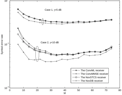
Fig. 1 examines the SERs of the receivers for different values ofM. One sees that the SERs
of the receivers decrease as M increases, up to a certain threshold. Then, the SERs of the
receivers increase asM increases. This is expected. WhenM increases, the receiver has a more
accurate channel estimate, but it also suffers from allocating more power to the pilot symbols.
At some point where the channel estimate is accurate enough, increasingM will mainly reduce
useful power without achieving worthwhile improvement in the channel estimation and, thus,
overall cause performance degradation. Comparing the NovSTCS receiver with the ConvML
and ConvMMSE receivers, one sees that the NovSTCS receiver is only slightly better than the
ConvML and ConvMMSE receivers. Also, one notes that the NovDB receiver has an obvious
performance gain over the ConvML and ConvMMSE receivers. This performance gain increases
4.75% of the total power for 16-QAM and 20% of the total power for QPSK.
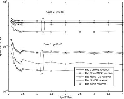
Fig. 2 shows the SERs of the receivers for different channel correlations. One sees that the
SER curves resemble the curve of a Bessel autocorrelation function. This is because a Bessel
correlation model is assumed and the receiver performs the best when the channel correlation is
the smallest. The SERs of the receivers vascillate slightly asdt/λordr/λincrease. Comparing
the NovSTCS receiver with the ConvML and ConvMMSE receivers, one sees that the NovSTCS
receiver is slightly better. Also, the NovDB receiver outperforms the ConvML and ConvMMSE
receivers as well as the NovSTCS receiver, which agrees with the previous observations from
Fig. 1. We will usedt/λ=dr/λ= 0.5next.
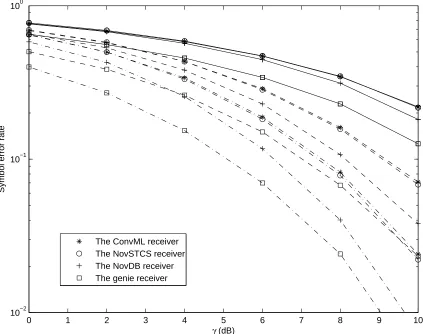
Fig. 3 compares the receiver performances in Case 1 for different values of r at different
SNRs. The performances of the receivers improve when r increases. In all the cases, the
NovSTCS receiver is slightly better than the ConvML receiver, and the NovDB receiver has
an obvious performance gain over the ConvML receiver and the NovSTCS receiver. The
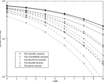
perfor-mance gain increases asr increases. Fig. 4 examines the receiver performances in Case 2 for
different values of r. In this case, the ConvML receiver performs the worst. The ConvMMSE
receiver outperforms the ConvML receiver, as it uses extra knowledge of the covariance matrix
and the mean channel matrix of the true channel gain. The NovSTCS receiver is slightly better
than the ConvMMSE receiver. The NovDB receiver performs the best among all the practical
receivers studied. Moreover, the performance gain increases when r increases or the SNR
in-creases. Comparing Fig. 3 with Fig. 4, one sees that the NovDB receiver in Case 2 performs
slightly better than that in Case 1, as expected, since Case 2 assumes more knowledge of the
channel statistics.
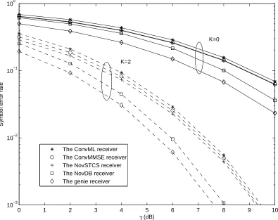
Figs. 5 and 6 show the SERs of the receivers in Case 1 and Case 2, respectively, for different
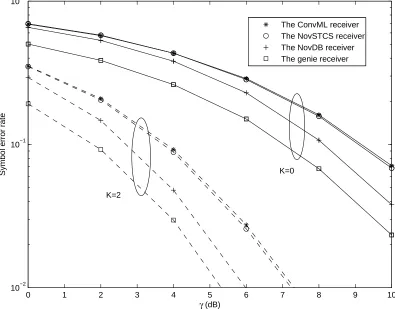
values of the Ricean K factor. From these figures, one sees that the receiver performances
improve when the value ofK increases. This is expected, as a larger value ofK corresponds
receivers. The performance gain increases when the value ofKincreases or the SNR increases.
This implies that the performance gains of the NovDB receiver over other receivers observed in
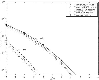
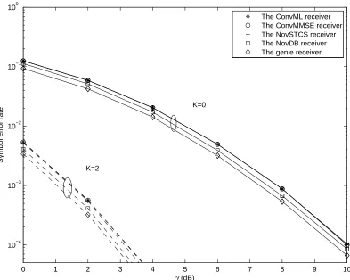
Figs. 1 to 4 are also achievable whenK > 0. Figs. 7 and 8 show the SERs of the receivers in
Case 2 for QPSK signaling. In general, the receivers using QPSK signaling perform better than
those using 16-QAM, under the same conditions. Also, one sees that the performance gains of
the NovDB receiver with QPSK are smaller than the corresponding gains with 16-QAM.
VI. CONCLUSIONS
Novel ML receivers for space-time coded MIMO systems with Gaussian channel estimation
errors have been derived. Numerical results have shown that the overall performance of the
system depends on several design parameters including the number of pilot symbols, the channel
correlation, the number of antennas, the Ricean K factor and the signaling scheme. Future work
includes an examination of new receivers for other MIMO systems with estimation errors.
REFERENCES
[1] S.N. Diggavi, N. Al-Dhahir, A. Stamoulis and A.R. Calderbank, ”Great expectations: the value of spatial diversity in
wireless networks,”P. IEEE, vol. 92, pp. 219-270, Feb. 2004.
[2] G. Foschini, ”Layered space-time architecture for wireless communication in a fading environment when using multiple
antenna elements,”Bell Labs Techn. J., vol. 1, pp. 41-59, Sept. 1996.
[3] S.M. Alamouti, ”A simple transmitter diversity scheme for wireless communications,”IEEE J. Select. Areas Commun.,
vol. 16, pp. 1451-1458, Oct. 1998.
[4] V. Tarokh, H. Jafarkhani and A.R. Calderbank, ”Space-time block codes from orthogonal designs,”IEEE Trans. Info.
Theo., vol. 45, pp. 1456-1467, July 1999.
[5] A. Lapidoth and S. Shamai, ”Fading channels: how perfect need ”perfect side information” be?,”IEEE Trans. Info. Theo.,
vol. 48, pp. 1118-1134, May 2002.
[6] M. Medard, ”The effect upon channel capacity in wireless communications of perfect and imperfect knowledge of the
channel,”IEEE Trans. Info. Theo., vol. 46, pp. 933-946, May 2000.
[7] D. Samardzija and N. Mandayam, ”Pilot-assisted estimation of MIMO fading channel response and achievable data rates,”
IEEE Trans. Signal Processing, vol. 51, pp. 2882-2890, Nov. 2003.
[8] T. Yoo and A. Goldsmith, ”Capacity and power allocation for fading MIMO channels with channel estimation error,”IEEE
[9] P. Kyritsi, R.V. Valenzuela and D.C. Cox, ”Channel and capacity estimation errors,”IEEE Commun. Lett., vol. 6, pp.
517-519, Dec. 2002.
[10] L.L. Chong and L.B. Milstein, ”The effects of channel estimation errors on a space-time spreading CDMA system with
dual transmit and dual receive diversity,”IEEE Trans. Commun., vol. 52, pp. 1145-1151, July 2004.
[11] R. Narasimhan, ”Error propagation analysis of V-BLAST with channel-estimation errors,”IEEE Trans. Commun., vol. 53,
pp. 27-31, Jan. 2005.
[12] T. Weber, A. Sklavos and M. Meurer, ”Imperfect channel-state information in MIMO transmission,”IEEE Trans.
Com-mun., vol. 54, pp. 543-552, Mar. 2006.
[13] P. Garg, R.K. Mallik and H.M. Gupta, ”Performance analysis of space-time coding with imperfect channel estimation,”
IEEE Trans. Wireless Commun., vol. 4, pp. 257-265, Jan. 2005.
[14] S.A. Zummo and W.E. Stark, ”Error probability of coded STBC systems in block fading environments,”IEEE Trans.
Wireless Commun., vol. 5, pp. 972-977, May 2006.
[15] E. Baccarelli and M. Biagi, ”Performance and optimized design of space-time codes for MIMO wireless systems with
imperfect channel estimates,”IEEE Trans. Signal Processing, vol. 52, pp. 2911-2923, Oct. 2004.
[16] D.V. Duong and G.E. Oien, ”Optimal pilot spacing and power in rate-adaptive MIMO diversity systems with imperfect
CSI,”IEEE Trans. Wireless Commun., vol. 6, pp. 845-851, Mar. 2007.
[17] E. Baccarelli, M. Biagi and C. Pelizzoni, ”On the information throughput and optimized power allocation for MIMO
wireless systems with imperfect channel estimation,”IEEE Trans. Signal Processing, vol. 53, pp. 2335-2347, July 2005.
[18] X. Wang and J. Wang, ”Effect of imperfect channel estimation on transmit diversity in CDMA systems,”IEEE Trans. Vehi.
Technol., vol. 53, pp. 1400-1412, Sept. 2004.
[19] V. Tarokh, A. Naguib, N. Seshadri and A.R. Calderbank, ”Space-time codes for high data rate wireless communication:
performance criteria in the presence of channel estimation errors, mobility, and multiple paths,”IEEE Trans. Commun.,
vol. 47, pp. 199-207, Feb. 1999.
[20] G. Taricco and E. Biglieri, ”Space-time decoding with imperfect channel estimation,”IEEE Trans. Wireless Commun.,
vol. 4, pp. 1874-1888, July 2005.
[21] Y. Chen and N.C. Beaulieu, ”Novel diversity receivers in the presence of Gaussian channel estimation errors,”IEEE Trans.
Wireless Commun., vol. 5, pp. 2022-2025, Aug. 2006.
[22] S. Kay,Fundamentals of Statistical Signal Processing: Estimation Theory. Upper Saddle River, NJ: Prentice-Hall, 1993.
[23] D.-S. Shiu, G.J. Foschini, M.J. Gans and J.M. Kahn, ”Fading correlation and its effect on the capacity of multelement
antenna systems,”IEEE Trans. Commun., vol. 48, pp. 502-513, Mar. 2000.
[24] T.-A. Chen, M.P. Fitz, M.P. Zoltowski, W.-Y. Kuo and J.H. Grimm, ”A space-time model for frequency nonselective
Rayleigh fading channels with applications to space-time modems,”IEEE J. Select. Areas Commun., vol. 18, pp.
0 10 20 30 40 50 60 70 80 10−2
10−1 100
M
Symbol errror rate
The ConvML receiver The ConvMMSE receiver The NovSTCS receiver The NovDB receiver Case 1, γ=5 dB
[image:23.595.113.516.228.540.2]Case 2, γ=10 dB
Fig. 1. Symbol error rates of receivers for different values ofM when r = 4, dt
λ =
dr
λ = 3,
0 0.5 1 1.5 2 2.5 3 3.5 4 10−2
10−1 100
d t/λ or dr/λ
Symbol error rate
The ConvML receiver The ConvMMSE receiver The NovSTCS receiver The NovDB receiver The genie receiver Case 2, γ=5 dB
[image:24.595.118.513.222.539.2]Case 1, γ=10 dB
Fig. 2. Symbol error rates of receivers for different values of dt
λ or
dr
λ whenr = 4,M = 20,
0 1 2 3 4 5 6 7 8 9 10
10−2
10−1
100
γ (dB)
Symbol error rate
[image:25.595.90.513.203.537.2]The ConvML receiver The NovSTCS receiver The NovDB receiver The genie receiver
Fig. 3. Symbol error rates of receivers in Case 1 forr = 2(solid line),r= 4(dashed line), and r= 6(dash-dotted line), when dt
λ =
dr
0 1 2 3 4 5 6 7 8 9 10
10−2
10−1
100
γ (dB)
Symbol error rate
[image:26.595.91.512.204.537.2]The ConvML receiver The ConvMMSE receiver The NovSTCS receiver The NovDB receiver The genie receiver
Fig. 4. Symbol error rates of receivers in Case 2 forr = 2(solid line),r= 4(dashed line), and r= 6(dash-dotted line), when dt
λ =
dr
0 1 2 3 4 5 6 7 8 9 10 10−2
10−1 100
γ (dB)
Symbol error rate
The ConvML receiver The NovSTCS receiver The NovDB receiver The genie receiver
K=0
[image:27.595.117.512.228.537.2]K=2
Fig. 5. Symbol error rates of receivers in Case 1 forK = 0(solid line) and K = 2 (dashed
line) whenr= 4, dt
λ =
dr
0 1 2 3 4 5 6 7 8 9 10 10−3
10−2 10−1 100
γ (dB)
Symbol error rate
The ConvML receiver The ConvMMSE receiver The NovSTCS receiver The NovDB receiver The genie receiver
K=0
[image:28.595.118.513.224.537.2]K=2
Fig. 6. Symbol error rates of receivers in Case 2 forK = 0(solid line) and K = 2 (dashed
line) whenr= 4, dt
λ =
dr
0 1 2 3 4 5 6 7 8 9 10 10−4
10−3 10−2 10−1 100
γ (dB)
Symbol error rate
The ConvML receiver The ConvMMSE receiver The NovSTCS receiver The NovDB receiver The genie receiver
r=2
r=4
Fig. 7. Symbol error rates of receivers in Case 2 forr = 2(solid line) andr= 4(dashed line),
when dt
λ =
dr
[image:29.595.121.510.221.535.2]0 1 2 3 4 5 6 7 8 9 10 10−4
10−3 10−2 10−1 100
γ (dB)
Symbol error rate
The ConvML receiver The ConvMMSE receiver The NovSTCS receiver The NovDB receiver The genie receiver
K=0
[image:30.595.119.512.221.535.2]K=2
Fig. 8. Symbol error rates of receivers in Case 2 forK = 0(solid line) and K = 2 (dashed
line), whenr = 4, dt
λ =
dr