Fast-starts are bursts of high-energy swimming starting either from rest or during periods of steady swimming (Domenici and Blake, 1997). They are used in interactions between predator and prey and are presumably important determinants of survival and feeding success. Fast-starts are largely powered by the recruitment of the fast myotomal muscle since the required strain rate exceeds that of the slower-contracting red muscle fibres (Rome et al. 1988; Altringham and Johnston, 1990). Red and white muscle fibres are anatomically distinct in fish myotomes (Alexander, 1969) and so fast-starts provide a good system on which to model muscle action for biologically important behaviours.
Muscle power output is the product of force and its shortening velocity. Estimates of power output were originally derived from steady-state force–velocity relationships measured during isotonic shortening experiments (e.g. Weis-Fogh and Alexander, 1977). The mean muscle-mass-specific power output during a complete contraction cycle was estimated in this way to be 80 W kg−1for insect synchronous flight muscle (Ellington, 1985). During the dynamic situation of muscle contraction found in most biological behaviours, however, quasi-steady predictions do not account for the whole muscle performance. The timing of muscle activity relative to
its movement plays a crucial role in determining muscle performance. Maximum power production during a cyclical movement requires the muscle to be fully active during shortening but fully relaxed during lengthening. However, neither activation nor deactivation occurs instantaneously. Muscle force is also modulated by shortening deactivation (Edman, 1980; Ekelund and Edman, 1982) and active prestretch (Edman et al. 1978a,b, 1982).
Muscle performance has been modelled for fish using data on activation times and ultrastructure coupled to steady force–velocity characteristics (van Leeuwen et al. 1990; van Leeuwen, 1992). These methods have been used to predict muscle function at different longitudinal positions, but not the absolute power output.
The effect of muscle movement can be incorporated into muscle force measurements by using work-loop techniques where isolated fibres are subjected to cyclical length changes whilst the force production is measured. This approach was developed by Machin and Pringle (1959) for asynchronous insect muscle, applied to synchronous insect muscle by Josephson (1985) and first used on fish by Altringham and Johnston (1990). Mean muscle-mass-specific power outputs during complete work loops have been measured at 130 W kg−1 Printed in Great Britain © The Company of Biologists Limited 1998
JEB1200
Fast-starts associated with escape responses were filmed at the median habitat temperatures of six teleost fish: Notothenia coriiceps and Notothenia rossii (Antarctica), Myoxocephalus scorpius (North Sea), Scorpaena notata and
Serranus cabrilla (Mediterranean) and Paracirrhites
forsteri (Indo-West-Pacific Ocean). Methods are presented for estimating the spine positions for silhouettes of swimming fish. These methods were used to validate techniques for calculating kinematics and muscle dynamics during fast-starts. The starts from all species show common patterns, with waves of body curvature travelling from head to tail and increasing in amplitude. Cross-validation with sonomicrometry studies allowed gearing ratios between the red and white muscle to be calculated. Gearing ratios must decrease towards the tail with a corresponding change in muscle geometry, resulting in similar white
muscle fibre strains in all the myotomes during the start. A work-loop technique was used to measure mean muscle power output at similar strain and shortening durations to those found in vivo. The fast Sc. notata myotomal fibres produced a mean muscle-mass-specific power of 142.7 W kg−1 at 20 °C. Velocity, acceleration and
hydrodynamic power output increased both with the travelling rate of the wave of body curvature and with the habitat temperature. At all temperatures, the predicted mean muscle-mass-specific power outputs, as calculated from swimming sequences, were similar to the muscle power outputs measured from work-loop experiments.
Key words: fast-start, skeletal muscle, muscle power output, fish, swimming.
Summary
Introduction
MUSCLE POWER OUTPUT LIMITS FAST-START PERFORMANCE IN FISH
JAMES M. WAKELING* ANDIAN A. JOHNSTON
Gatty Marine Laboratory, School of Environmental and Evolutionary Biology, University of St Andrews, St Andrews, Fife KY16 8LB, Scotland
*e-mail: [email protected]
at 40 °C for the hawkmoth Manduca sexta (Stevenson and Josephson, 1990) and 135 W kg−1 at 35 °C for the lizard
Dipsosaurus dorsalis (Swoap et al. 1993). Work-loop
experiments on fish have been refined further by taking direct measurements of the in vivo muscle length changes and activation patterns using sonomicrometry and electromyography techniques and then imposing these shortening regimes on isolated fibres in vitro (Franklin and Johnston, 1997). These techniques have resulted in fish mean muscle-mass-specific power outputs being measured between 18.1 W kg−1 at 0 °C for Notothenia coriiceps (Franklin and Johnston, 1997) and 75.7 W kg−1at 15 °C for Myoxocephalus
scorpius (G. Temple, personal communication).
Muscle power output can be estimated from the whole-body performance of an animal. During most locomotory activities, the power required for motion must be generated by the muscles. Estimates of the hydrodynamic power requirements for swimming can thus be used to predict a minimum value for fish muscle power output. Frith and Blake (1995) estimated a muscle-mass-specific power output of 300 W kg−1at 10 °C for fast-starts in pike Esox lucius using such an approach. This prediction is higher than any fish muscle power output measured to date.
The aim of the present study was to compare estimates of muscle power output from work-loop measurements on isolated fibres (both from this study and drawn from the
literature) with predictions made from whole-body swimming performance during fast-starts. The species used in this study were drawn from a range of habitat temperatures. It is known that increases in temperature correlate with increased muscle power output for a range of phyla (Stevenson and Josephson, 1990; Josephson, 1993). Greater muscle power availability should drive higher fast-start accelerations and thus higher velocities. We thus hypothesised that fast-start performance, in terms of velocity and acceleration, would be lower for colder species and that increases in fast-start performance would mirror increases in the muscle power available at higher temperatures. This study also set out to quantify the muscle kinetics for these starts to determine whether differences in fast-start performance were related to differences in muscle shortening.
Materials and methods
Fish
The marine fish Notothenia coriiceps (Nybelin), Notothenia
rossii (Richardson), Myoxocephalus scorpius (L.), Scorpaena notata (L.), Serranus cabrilla (L.) and Paracirrhites forsteri
[image:2.609.41.561.413.696.2](Bloch and Schneider) were used for this study. The Antarctic notothenioids were caught by the British Antarctic Survey around Signy Island, South Orkneys, in 1995; the short-horn sculpin M. scorpius were caught in St Andrews Bay, Scotland,
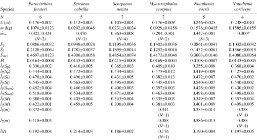
Table 1. Morphological body parameters of the fish used in this study
Paracirrhites Serranus Scorpaena Myoxocephalus Notothenia Notothenia
Species forsteri cabrilla notata scorpius rossii coriiceps
N 6 5 7 7 5 4
L (m) 0.176±0.007 0.112±0.005 0.105±0.004 0.176±0.009 0.246±0.025 0.238±0.010
m (kg) 0.1076±0.0123 0.0202±0.0048 0.0231±0.0024 0.0929±0.0158 0.1578±0.0415 0.1585±0.0155
mˆm 0.322, 0.424 0.470 0.363±0.008 0.294, 0.301 0.447±0.001 0.300*
(N=2) (N=1) (N=4) (N=2) (N=3)
Sˆp 0.0886±0.0032 0.0948±0.0028 0.1195±0.0036 0.1402±0.0036 0.0861±0.0041 0.1032±0.0032
Sˆl 0.2120±0.0064 0.1781±0.0037 0.1895±0.0014 0.1252±0.0016 0.1432±0.0061 0.1566±0.0015
Sˆwet 0.4697±0.0123 0.4306±0.0058 0.4854±0.0074 0.4173±0.0048 0.3603±0.0146 0.4080±0.0054
Mˆ 0.0164±0.0008 0.0143±0.0003 0.0215±0.0008 0.0169±0.0004 0.0108±0.0007 0.0143±0.0005
lˆ1(Sp) 0.390±0.002 0.410±0.005 0.365±0.003 0.409±0.010 0.355±0.008 0.368±0.004
lˆ2(Sp) 0.444±0.001 0.472±0.005 0.434±0.005 0.473±0.012 0.419±0.009 0.427±0.006
lˆ1(Sl) 0.478±0.004 0.496±0.007 0.431±0.005 0.382±0.013 0.472±0.007 0.470±0.002
lˆ2(Sl) 0.545±0.004 0.563±0.007 0.495±0.006 0.445±0.014 0.540±0.007 0.540±0.002
lˆ1(Swet) 0.452±0.004 0.466±0.005 0.406±0.003 0.397±0.003 0.428±0.005 0.430±0.002
lˆ2(Swet) 0.518±0.004 0.534±0.005 0.471±0.004 0.463±0.004 0.498±0.006 0.498±0.003
lˆ1(M) 0.380±0.001 0.405±0.004 0.343±0.004 0.335±0.003 0.349±0.007 0.357±0.004
lˆ2(M) 0.422±0.001 0.459±0.005 0.390±0.004 0.381±0.003 0.401±0.009 0.409±0.005
lˆ1(m) 0.372±0.004 0.344 0.335±0.014 0.338
(N=1) (N=1)
lˆ2(m) 0.418±0.004 0.388 0.386±0.013 0.388
(N=1) (N=1)
lˆ(I) 0.192±0.004 0.214±0.003 0.186±0.002 0.176 0.190±0.004 0.197±0.005
(N=1)
Values are mean ±S.E.M., where N is the number of values unless indicated otherwise. Where N=1 or 2, one or both values are given. See symbols list for definitions of parameters.
UK, in 1995; the Mediterranean scorpionfish Sc. notata and comber Se. cabrilla were caught and supplied by the Zoological Station, Naples, Italy, in 1997; the tropical black-sided hawkfish P. forsteri were imported from the Hawaiian Islands in 1996. In their natural habitats, these fish experience the following temperature ranges: Signy Island, Antarctica (60°43′S, 45°36′W), −2 to 1 °C; North Sea, 4–17 °C; Mediterranean Sea, 10–28 °C; Hawaiian Islands, 24–26 °C. Temperature-controlled aquaria in our laboratory maintained the fish at their respective median temperature, i.e. N. coriiceps and N. rossii at 0 °C, M. scorpius at 15 °C, Sc. notata and Se.
cabrilla at 20 °C and P. forsteri at 25 °C. The numbers and
sizes of the fish can be found in Table 1. Fish were held at these temperatures for at least 4 weeks prior to observations and were fed daily on krill, chopped squid or shrimp.
Kinematic parameters
Fast-starts were filmed in a static tank with dimensions 2.0 m×0.6 m×0.2 m (length × width × height). The water temperature was controlled at the acclimation temperature for the species being filmed. Starts were elicited by visual or tactile stimuli; for N. coriiceps and M. scorpius, starts were elicited by a tap to the caudal peduncle with a rod, whilst the other species were startled by the rod approaching from the front. The tank was lit from underneath by a bank of five 70 W fluorescent strip lights. Overhead images of the fish were filmed via a mirror positioned at 45 ° above the tank. Fish silhouettes were recorded on 16 mm Ilford HP5 film on a NAC Inc., Japan, E-10 high-speed ciné camera at 500 frames s−1 using a 29 mm lens. The light path between the fish and the film was 2.6 m, and the frame diagonal was typically four fish lengths long. Film sequences were digitized on a NAC 160F film motion image analyser. The standard error of digitizing a reference point on sequential frames corresponded to 0.001 body lengths. Timing for the sequences was calibrated by means of a light strobing at 100 Hz within the camera. All fast-start sequences that did not show tilting or rolling of the fish were analysed.
The x,y coordinates of 10 equidistant points running from snout to tail along the spine were digitized by eye for each ciné frame. The centre of mass for a straight stretched fish lies at a distance lˆ1(m) along the spine from the snout where lˆ1(m) is the non-dimensional radius of the first moment of mass (see equation A14, Appendix). Using the procedures described in the Appendix (equations A30–A32), the x,y coordinates of this point on the spine were calculated. This ‘quick’ method was validated against a more rigorous method involving computation of the spine position from the fish outlines (equations A18–A29). Similarly, a detailed method is given in the Appendix for quantifying fish morphology. Validation of the various techniques is described more fully in a later section.
Velocity and acceleration
Velocity V and acceleration A were determined from the displacement of the centre of mass of the fish during the first complete tailbeat of each start. Fast-starts involve both
unsteady velocities and accelerations, and their estimates are very sensitive to the manner in which the data are smoothed. This study fitted cubic regressions to subsequent sections of the position data in order to smooth the estimates of position. This method is analogous to fitting a moving average (Webb, 1978; Frith and Blake, 1995; Harper and Blake, 1989, 1990; Domenici and Blake, 1991; Kasapi et al. 1992; Beddow et al. 1995; Franklin and Johnston, 1997) with the difference that we took a cubic fit where traditionally a linear fit has been used.
The position data gave a series of N values where there were
N frames in the sequence. For each frame j, a ‘smooth’ estimate
of the position was given by the value h(j), where h(x) was the least-squares cubic regression for the x coordinates in frames
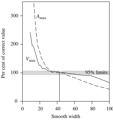
[image:3.609.340.539.394.605.2]j−n to j+n and the smooth width was 2n+1. The velocity and acceleration for each frame were given by the first and second differentials, respectively, of h(j) with respect to time. Smoothed results were not calculated for the first and last n frames in the sequence. The procedure was repeated for the data in the y direction. Where there was a maximum or minimum to the data, then the cubic fit would accurately match the peak values. The smooth width was still important; if it was too small, then peak values would contain digitizing uncertainty, and if it was too large then it would encompass several peaks and thus be unable to give a good fit to each one. The effect of the smooth width on the maximum velocity
Fig. 1. Increasing the width of sequential portions of the cubic fit to the position data results in a decrease in the estimated maximum velocity Vmax and acceleration Amax. The smooth width of 43 for this
sequence (vertical line) results in a fit where the digitizing errors have been smoothed, but the overall displacement data are preserved. The standard error of the smoothed positions from the raw data is 0.0015L (N=150), where L is total length for this smooth width. The standard error of the position of a reference point digitized from sequential frames is 0.00123L (N=80). The smooth width of 43 can thus be justified from the digitizing accuracy. The 95 % confidence limits of the velocity and acceleration data are shown by the shaded region.
0 100 200 300
0 20 40 60 80 100
Amax
Vmax
95% limits
Smooth width
Vmaxand acceleration Amaxestimates can be seen in Fig. 1. As the smooth width increases, there is a sharp initial drop as the digitizing errors are smoothed. Next occurs a relatively level portion with the peaks and troughs being accurately fitted. Finally, the values of maximum velocity and acceleration decrease and the increasing smooth width causes over-smoothing. Values for the smooth width which gave accurate fitting of the maxima coincided with those that resulted in the standard error of the smoothed position data from the raw position data matching the standard error of repeatedly digitizing a point from the film (Fig. 1). Thus, we have confidence that the velocity and acceleration estimates were based on the correct degree of smoothing.
The correct value for the smooth width depends on the digitizing accuracy. The correct smooth width also depends on the number of digitized frames per tailbeat or similar event which produces a fluctuation in acceleration. Smooth width was estimated independently for each species analysed here.
Velocity and acceleration were determined for both the x and
y directions, and the resultant was calculated as the total value.
The acceleration estimate thus included the centripetal acceleration and did not necessarily take the same direction as the velocity. The tangential acceleration, which is the component of acceleration in the velocity direction, was also calculated. Rotational velocity and acceleration were estimated from the change in yaw angle in an analogous manner to the translational values, where yaw is the angle between the velocity vector and the spine at the position of the centre of mass ψ (see equation A33).
Length-specific velocity Vˆ and acceleration Aˆ were calculated relative to the total body length L, where Vˆ=V/L and
Aˆ=A/L, respectively.
Power requirements during swimming
Fast-starts are rapid acceleration events, and during the start the useful power Puse expended to move in a tangential direction can be approximated by the inertial power Piner, where:
and m is the body mass, mais the added mass of water that must be accelerated with the body, V is the velocity, and A is the acceleration. The added mass of water that moves with a fish during fast-starts has been estimated as ma=0.2m (Webb, 1982).
The inertial power as described in equation 1 is that required for linear accelerations. The inertial power required for a rotational acceleration Piner,rot is given by a second relationship:
where I is the moment of inertia of the fish [I=r2(m+m
a)] about the centre of rotation, ω is the angular velocity, a is the angular acceleration, and r is the distance of the centre of mass of the fish from that centre of rotation. The tangential velocity V and
acceleration A are the following functions of the rotational values: ω=V/r and a=A/r, respectively. Substituting the values for I, ω and a into equation 2 reduces the expression for Piner,rot to the same as the translational inertial power Pineras given in equation 1. Inertial power was thus calculated from tangential velocity and acceleration regardless of whether the fish followed a linear or turning course.
Translational inertial power estimates consider the acceleration of the centre of mass of the fish in the tangential direction. The centre of mass does not necessarily occur at a position along the spine; as a fish bends into a C-shape, the centre of mass moves away from the spine to lie within the space enclosed by the ‘C’. Weihs (1973) showed the fish centre of mass in its actual position, moving away from the spine during bending. Later studies, however, take it to occur at the same point along the spine as in a straight-stretched fish. The position vector q describing the true centre of mass is estimated by the mean position of 10 segments of the fish when each segment is given a weighting of its mass (volume):
s(i) is the position vector for the centre of each segment (see equations A30–A32), vi is the volume for that segment as
calculated for the straight fish (equation A9), and M is the total volume of the fish (equation A10). The effect of taking the actual centre of mass for the fish as opposed to that occurring along the spine can be seen in Fig. 2. Much of the initial movement of the spine occurs because the fish bends and does not represent a net displacement of the centre of mass. The course of the centre of mass is much straighter than that shown by the centre as positioned on the fish spine.
Useful hydrodynamic power Puse (≈Piner) is expended to propel the fish in its direction of travel. However, as the body flexes, there is lateral motion; the total hydrodynamic power Ptis the total power expenditure during the movement both in the direction of travel and perpendicular to that direction. The hydrodynamic efficiency η is the ratio of the useful power to the total power:
Hydrodynamic efficiency has been estimated for a number of pike (Esox lucius) fast-starts by Frith and Blake (1995), who give values of η which relate Ptto useful hydrodynamic power and additionally give values of Piner calculated for the same sequence. The mean η for the pike fast-starts which related Pinerto Ptis 0.31, and this value was used for the starts in the present study. Specific differences in kinematics may lead to specific differences in η; however, this will only be resolved when detailed hydrodynamic analyses of fast-starts are applied to a range of species.
During swimming, the fish may rotate so that it does not face t
iner P P =
η . (4)
M v i i
i
∑
= =
10
1
) (
s
q . (3)
a I
Piner,rot =ω , (2)
VA m m P
its direction of travel. Yaw is taken as the angle between the velocity and the tangent to the spine at its centre of mass, lˆ1(m). Angular accelerations in yaw must be accompanied by turning torques, and the power for these can be calculated from equation 2, where I is the moment of inertia of the fish (equations A15–A17), and ω and a are the angular velocity and acceleration, respectively, of the yaw. The moment of inertia is taken from straight-stretched bodies and so will be an overestimate for that from C-shaped postures. Nonetheless, the mean power expended for the yaw in 10 fast-start sequences was a mere 0.001 % of the inertial power expended for those starts. The costs of yawing were thus ignored during this analysis.
Mean inertial power was integrated for the duration of the
first complete muscle shortening cycle (as seen in the curvature plot, see Fig. 7). In almost all cases, the inertial power was positive. Negative inertial power did occasionally occur, corresponding to fish decelerations. However, assuming that such decelerations are passive during fast-starts, the mean power requirements were calculated solely from the positive contributions.
Muscle strain
White muscle strain εwand activation was measured directly in N. rossii and P. forsteri during fast-starts using the sonomicrometry and electromyography (EMG) method described by Franklin and Johnston (1997). Pairs of sonomicrometry crystals implanted into the myotomal muscle measure the muscle length from the velocity of sound transmission between the crystals. Anaesthesia was initiated with a 1:5000 (m/v) solution of bicarbonate-buffered MS222 (ethyl m-aminobenzoate) and maintained by irrigation of the gills with a 1:3 dilution of this solution during surgery. Surgery was performed in a constant-temperature room set to the acclimation temperature of the respective species. Sonomicrometry and EMG measurements were taken from superficial rostral fibres at 0.35L, where L is the fish total length. For both species, previous dissections on dead specimens had confirmed that crystal positioning was in an alignment parallel to the surrounding fibres. Sonomicrometry data were also available for two other species recorded from our laboratory: N. coriiceps (Franklin and Johnston, 1997) and
M. scorpius (G. Temple, unpublished data).
Muscle strain was predicted additionally from the shape and curvature of the body. The strain at the edge of the planform fish silhouette corresponds to the strain at the lateral line of the fish. This is the region where the red, aerobic fibres occur. Where muscle fibres run parallel to the spine, then their strain
ε can be calculated using trigonometry as:
where bˆ (=b/L) is the length-specific distance from the spine to those fibres (half the width of the fish: see Appendix for methods of quantifying fish shape), and cˆ is the length-specific curvature of the spine at that location (equation A35). If the orientation of the red fibres is not parallel to the spine, then a correction should be made when calculating the strain (van Leeuwen et al. 1990) as oblique fibres undergo smaller strains than parallel fibres.
The white fibres run in a helical arrangement deeper within the fish than do the red fibres (Alexander, 1969). This helical arrangement results in the strain being similar for white fibres at different depths; however, this strain may be less than that for the adjacent red fibres. The gearing ratio is the ratio of the red fibre strain to the white fibre strain for a given curvature of the body and was predicted to take a value of approximately 4 (Alexander, 1969). In the present study, the gearing ratio λ was estimated as the ratio of the mean white fibre strain ε¯wfor a series of fast-starts (as measured using the sonomicrometry
ε =bc , (5)$$
Time (s)
0.05 0.10 0.15 0.20 50
0 0
100 150 2 4
A
(s
−
2)
V
(s
−
1) B
0 0.048
0.096 0.240
0.144
0.192 A
Fig. 2. (A) Spine positions for Myoxocephalus scorpius. Arrowheads indicate the snout, circles denote the position of the centre of mass as located on the spine, and numbers indicate the time (s) at which each image occurred. The solid blue line marks the displacement of the true centre of mass, the solid red line is the displacement of the centre of mass as located on the spine, and the dashed green line shows the displacement of the snout. (B) Non-dimensional velocity
Vˆ and acceleration Aˆ estimates for the start shown in A. The blue
[image:5.609.54.293.67.414.2]technique) to the corresponding mean red fibre strain ε¯red (as calculated by equation 5), where:
Deviations in red fibre orientation from parallel to the spine are ignored. This results in a slight overestimate in the gearing ratio. However, this error is not propagated into estimates for the white muscle strain.
Validation of the techniques
A set of six P. forsteri fast-starts was used to validate the quicker method of digitizing the spine position ‘by eye’ against the full method involving equations A18–A29 in the Appendix. If the calculated spine position is considered to be correct, then the position judged by eye resulted in mean errors of 1.8 % and 1.5 % increase in Vˆmax and lateral line strain, respectively, and of 0.3 % and 1.1 % decrease in Aˆmaxand P–iner, respectively. The errors in velocity and acceleration, and therefore power, are smaller than those introduced by the smoothing technique (see Fig. 1), and so digitizing the spine by eye does not increase the uncertainty of the results. The errors for the strain estimates that are introduced by digitizing the spine by eye are similarly very small. If the mean white muscle strain ε¯w is set by a mean gearing ratio from equation 6, then there will be no difference between ε¯w for the two methods of estimating spine position. If the white muscle strain is set by an arbitrary gearing ratio, as has been the case for some other studies, then the difference between the two methods will be smaller than any error involved with the choice of gearing ratio.
In vitro muscle mechanics
Muscle contractile properties were determined for live fast fibre preparations from Sc. notata using the protocols described by Johnston et al. (1995), but with the following modifications. Preparations were isolated from the anterior abdominal muscles at a rostal position 0.35L along the fish. Fibres were dissected in a Ringer’s solution with the following composition (in mmol l−1): NaCl, 143; sodiun pyruvate, 10; KCl, 2.6; MgCl2, 1.0; NaHCO3, 6.18; NaH2PO4.2H2O. 3.2; Hepes sodium salt, 3.2; Hepes, 0.97; pH 7.3 at 20 °C. Both dissections and measurements were carried out at 20 °C. The length of the preparation was set to give maximal twitch. Preparations were frozen in isopentane cooled to −159 °C with liquid nitrogen. Frozen sections, 10µm thick, were cut at several points along the preparation and stained for myosin ATPase activity (Johnston et al. 1974). Muscle mass was calculated from its volume (the product of length and cross-sectional area) assuming a density of 1060 kg m−3(Mendez and Keys, 1960). Maximum contraction velocity V0was determined using the slack test (Edman, 1979); fibres were given a step release during the plateau phase of an isometric tetanus sufficient to abolish force. V0is the slope of the linear regression of step length against the time taken to redevelop force (6–8 step changes). Work-loop experiments were performed using single
sine waves. Cycle periods were tested in a range around 92 ms, the mean cycle period for the initial tailbeat as measured from ciné film. Fibre-length-specific peak-to-peak strain amplitude was set to 0.07, corresponding to that used by M. scorpius of similar size; the justification for this assumption is that the kinematics of these two species are similar (see Fig. 6). Two to three stimuli were given at a frequency of 260 Hz, which was shown to yield maximum tetanic force in preliminary experiments. Stimuli started just before peak length, with a duty cycle of 71.5–139.5 °. The passive work done by unstimulated fibres was always less than 4 % of the total work and was subtracted from the total work in each case.
Statistics
Least-squares linear regression was performed on sets of data to test the dependence of each parameter on the predictor variable. The kinematic parameters describing velocity, acceleration and power were all heteroscedastic and so were only tested after logarithmic transformation. Reduced major axis (Model II) regression was performed where the predictor was a random variable (Rayner, 1985), i.e. the non-dimensional radius of the kth moment of volume lˆk(M) and
Piner.
A multivariate analysis of covariance tested the correlation between the kinematic parameters cˆ, εred, Uˆ and the fast-start performance parameters Vmax, Vˆmax, Amax, Aˆmax and Pinerwith the habitat temperature as a factor, where Uˆ is the length-specific velocity at which curvature travels along the body and
Vˆmax and Aˆmax are the length-specific maximum velocity and acceleration of the fish, respectively. The fast-start performance parameters and Uˆ were all log-transformed owing to their heteroscedastic nature.
Q10values were calculated from the slopes of least-squares linear regressions on log-transformed data for kinematic parameters and temperature. Q10values were calculated using the mean kinematic parameter for each and every species.
All statistical tests were considered significant at a 95 % confidence level.
Results
Body morphologies
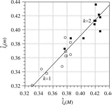
Length-specific fish chords are shown in Fig. 3. The various morphological parameters are given in Table 1 and shown in Figs 4 and 5 and provide a means to quantify differences between the shapes of the species. The non-dimensional radii of the moments of volume provide a good predictor of the dimensional radii of the moments of mass (Fig. 4). The non-dimensional radii of the moments of mass are predicted from the moments of volume by the following linear relationship:
where k takes a value of 1 or 2 for the first and second moments, respectively. The predicted radii of the moments of mass deviate from the relationship in equation 7 with a
033 . 0 ) ( ˆ 065 . 1 ) (
ˆ m = l M −
lk k , (7)
ε ε
w red
standard error of 0.0025 and with an error never more than 0.0207. Some of this variation is interspecific, with different species having different density distributions throughout their
body. Nonetheless, the centres of mass for straight-stretched fish can be estimated reliably from the centres of volume as measured using two orthogonal views of the fish alone.
The relationships between the non-dimensional radii of the moments of area and volume are shown in Fig. 5. They are analogous to series given for the shapes of insect wings (Ellington, 1984). Relationships between the parameters have not been explained and have been termed ‘laws of shape: rules that are obeyed even if the reasons for doing so are unknown’ (Ellington, 1984). These relationships do, however, provide a good way to quantify body shape, and discrete clusters of points highlight specific morphologies (Fig. 5).
The mean depth to slenderness of each species is given by the ratio Sˆl/Sˆp, where Sˆl and Sˆp are the non-dimensional longitudinal and planform areas, respectively (see equations A1–A4). In general, P. forsteri is a deep, slender fish, while M.
scorpius is the opposite extreme, wide and shallow. The
non-dimensional radii of the moments of longitudinal area, lˆ1(Sl) and
lˆ2(Sl), show distinct groups for each species. The two species ,
Sc. notata and M. scorpius, have the greatest proportion of
longitudinal area in their head region, with M. scorpius having the relatively deepest head. The length-specific estimate for the centre of mass lˆ1(M) is similarly most anterior for these two species. N. rossii also has a low value for lˆ1(M) because it has a having a relatively broad head, as shown by its low non-dimensional radii for the first and second moments of planform area lˆ1(Sp) and lˆ2(Sp).
Notothenia coriiceps Notothenia rossii
Myoxocephalus scorpius Scorpaena notata
Paracirrhites forsteri Serranus cabrilla
0 0.2 0.4 0.6 0.8 1
0.2 0 0.2
l
b
0 0.2 0.4 0.6 0.8 1
l 0.2
[image:7.609.79.536.69.380.2]0 0.2 0.2 0 0.2
Fig. 3. Length-specific body chord bˆ as a function of the non-dimensional length lˆ for the six species in this study.
Fig. 4. The non-dimensional radii of the first and second moments of mass lˆk(m) are predicted by the non-dimensional radii of the first and second moments of volume lˆk(M). Open circles, k=1; filled squares k=2. The line denotes the reduced major axis regression of lˆk(m) on lˆk(M) (see text for explanation), with r2=0.88, P=0.0003. The volume distribution of the fish body can thus be used as an estimate of the mass distribution.
0.32 0.34 0.36 0.38 0.40 0.42 0.44
0.32 0.34 0.36 0.38 0.40 0.42 0.44
lk
(m
)
lk(M) k=1
[image:7.609.76.267.477.657.2]There were no significant regressions between any of the mean morphological parameters and the habitat temperature, except one. The non-dimensional wetted area showed a significant positive regression with habitat temperature (r2=0.686, P=0.0418). However, wetted area affects viscous drag which, in turn, is a function of fish velocity. This study considers the initial moments of fast-starts where the velocity is low; therefore, the contribution of viscous drag is negligible and is ignored. For the purposes of this study, we will assume that habitat temperature has no significant effect on body morphology.
Fins are important for swimming, and their shape and area must be quantified for hydrodynamic analyses. However, such measurements are not required for the estimates of inertial power used in this study. Instead, this analysis concentrates on muscle action during swimming and so considers the shape of
the body which bounds the muscle. The non-dimensional muscle mass mˆmadditionally is given in Table 1.
Fast-start muscle dynamics
A characteristic body motion was used by all the species during their fast-starts. This body motion can be described by the mean maximum curvature and strain values for the range of body positions, and these are shown in Fig. 6. The fish initially undergo a strong bending, resulting in a ‘C’ or an ‘S’ body shape. There was a continuum of shapes between these two extremes. Often a rapid bending of the central body was accompanied by an inertial lag of the tail, resulting in a very slight ‘S’ shape at the tail. Consequently, starts were not pigeon-holed into categories during this analysis, and all forms are considered together.
The initial bending occurred as a wave of bending travelling
0.38 0.40 0.42 0.44 0.46 0.48 0.50 0.52
0.32 0.34 0.36 0.38 0.40 0.42 0.44 0.46
0.42 0.46 0.50 0.54 0.58 0.62
0.34 0.38 0.42 0.46 0.50 0.54
0.45 0.47 0.49 0.51 0.53 0.55
0.38 0.40 0.42 0.44 0.46 0.48
0.36 0.38 0.40 0.42 0.44 0.46 0.48
0.31 0.33 0.35 0.37 0.39 0.41 0.43
l1
(Sl
)
l1
(Sp
)
l2(Sp) l2(Sl)
l1
(Swet
)
l2(Swet)
l1
(M
)
[image:8.609.100.504.74.460.2]l2(M)
from head to tail (Fig. 7) with length-specific velocity Uˆ. Being a wave of bending, there are no discrete times when the fish is in a ‘C’ shape on either side. It is thus impossible to determine accurately the times for the classical stages of each start (Weihs, 1973). The cranium is a relatively rigid structure which does not bend significantly during the start. The tail, in contrast, is flexible and can bend considerably. The curvature thus increased along the fish to a position at approximately 0.6L, where it then remained relatively constant (Fig. 6). All body parameters are considered in the range 0.2–0.8L; however, in some species, such as M. scorpius, the stiff cranium extends beyond the 0.2L position and may influence the parameters at this location. In order to tidy subsequent plots (Fig. 7), the curvature and strain were set to decrease linearly
to zero between the extremes at 0L and 1L and the respective main body values at 0.2L and 0.8L.
[image:9.609.76.265.69.431.2]The strain εredis a function of both the local body chord and curvature. The chord decreases between 0.2L and 0.8L in all species, resulting in a general decrease in εred (Fig. 6). All species except N. rossii showed a reasonably constant strain between 0.3L and 0.5L, where the increase in curvature balances the decrease in chord; their strains then decrease towards the tail. N. rossii showed a linear decrease in εred from 0.3L to the tail. Despite M. scorpius having the greatest length-specific chord (Fig. 3), it did not show the highest εred because its body curvature was less than that of the notothenioids. Similarly, P. forsteri had the lowest mean εred despite it being one of the most slender fish (as shown by Sˆp; Table 1). Body curvature thus has a greater effect on εred than does body chord, and the strain at all positions along the fish increased with decreasing habitat temperature due to increasing curvature (Fig. 6).
Sonomicrometry data for fast-starts give mean white muscle peak-to-peak strains of 0.10, 0.20, 0.10 and 0.12 for N.
coriiceps (Franklin and Johnston, 1997), N. rossii (Fig. 8), P. forsteri (this study) and M. scorpius (G. Temple, personal
communication), respectively, at positions 0.35L, 0.36L, 0.40L and 0.35L, respectively. The gearing ratio λ is thus 4.09, 2.49, 2.07 and 2.39, respectively, for N. coriiceps, N. rossii, P.
forsteri and M. scorpius at these respective positions.
The predicted strain waves for each body position sometimes have broad peaks at maximum and minimum
1 3 5 7 9 11
0.1 0.2 0.3 0.4 0.5 0.6 0.7 0.8 0.9
0.05 0.15 0.25 0.35 0.45 0.55
0.1 0.2 0.3 0.4 0.5 0.6 0.7 0.8 0.9
l
c
εred
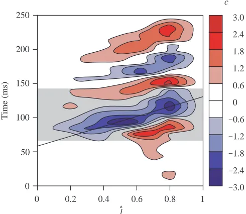
Fig. 6. The amplitude of the non-dimensional curvature cˆ increases with non-dimensional longitudinal body position lˆ during fast-starts. Peripheral strain εred, in contrast, decreases from its maximum in the mid-fish towards the tail owing to decreasing chord length. Mean values for all the starts for each species are plotted ±S.E.M. Symbols are as follows: open squares, Paracirrhites forsteri (N=14); open triangles, Serranus cabrilla (N=36); open circles, Scorpaena notata (N=38); filled circles, Myoxocephalus scorpius (N=15); filled triangles, Notothenia rossii (N=21); filled squares, Notothenia coriiceps (N=27).
0 50 100 150 200 250
2.4 1.8 1.2 0.6 0 0.6 1.2 1.8 2.4
c
0 0.2 0.4 0.6 0.8 1
l
Time (ms)
3.0
3.0
− −
−
−
[image:9.609.319.564.80.293.2]−
muscle length. Measuring contraction duration as the period from maximum to minimum length will thus contain uncertainty as to the exact start and end of the contraction. An artifically low, but more robust, estimate for the contraction duration is the muscle strain divided by the maximum strain rate, and these durations range from 63 ms for the Antarctic fish to 25 ms for the Hawaiian and Mediterranean fish. Sonomicrometry traces show that these values are typically 0.57 of the actual shortening period. Mean contraction durations are longer in the Antarctic than in the warmer-water species and have a Q10of 0.66. The mean contraction duration shows no significant regression with body position, i.e. contraction duration remains constant at all positions along the body. Caution should be used when comparing contraction durations between species because longer durations may reflect contraction over greater strains as well as contractions at slower rates.
In vitro muscle mechanics
The contractile properties for Sc. notata live fast fibres at 20 °C are summarised in Table 2. The maximum tetanic stress for Sc. notata of 239 kN m−2falls within the range of stress measured in other vertebrates i.e. from 241 kN m−2 for the dogfish Scyliorhinus canicula (Curtin and Woledge, 1988) to 151 kN m−2in the saithe Pollachius virens (Altringham et al. 1993).
The maximum fibre length-specific contraction velocity V0 as measured by the slack test is 13.2 s−1. Maximum length-specific contraction velocities as measured both by slack-test
methods and extrapolated from force–velocity relationships tend to increase with habitat temperature (Fig. 9) and V0for
Sc. notata falls within this range. The Q10 for maximum fish fast muscle length-specific contraction velocity is 2.2.
Fast-start performance
The different species showed characteristic styles of start.
M. scorpius and Se. cabrilla typically swam off in a direction
close to their original orientation, whereas the other species turned to a larger extent. During turning, there is a centripetal
0.05 0.10
0.05
0.10
w
200 400 600
[image:10.609.48.292.77.301.2]Time (ms)
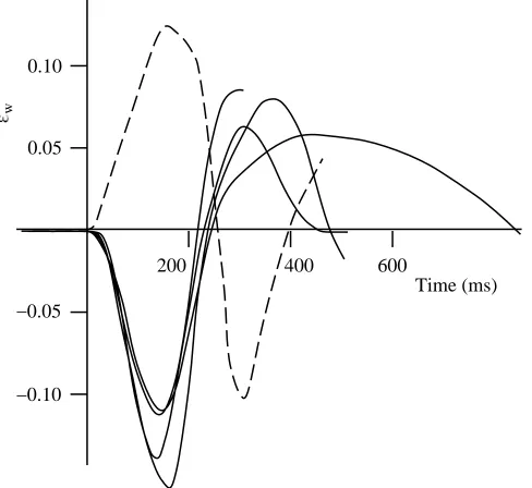
[image:10.609.314.561.97.291.2]Fig. 8. Strains εw in the rostral fast muscle fibres of one N. rossii individual for a series of fast-starts. Dashed and solid lines correspond to recordings from opposite sides of the body. Sonomicrometry crystals were positioned at a longitudinal position 0.36L from the snout, where L is the total length.
Table 2. Contractile properties for Scorpaena notata live
rostral fast fibre preparations at 20 °C
Contraction
type Parameter
Twitch Maximum stress (kN m−2) 163.62±17.67
Time to half-maximum force 9.32±0.73
(ms)
Time from maximum force to 10.05±0.36
half-relaxation (ms)
Tetanus Maximum stress (kN m−2) 239.18±16.72
Time to half-maximum force 13.43±0.66
(ms)
Time from maximum force to 30.49±1.81
half-relaxation (ms)
Slack test Maximum length-specific 13.17±3.47
contraction velocity, V0(s−1) (N=4)
Work loop Mean power output (W kg−1) 142.73±12.30
Mean ±S.E.M. (N=6 unless indicated otherwise).
Fig. 9. Fish fast muscle length-specific contraction velocity V0 as measured by both slack test and force–velocity methods versus habitat temperature. The open square is for Scorpaena notata from this study. Filled circles denote data for Notothenia coriiceps (1, 2) (Franklin and Johnston, 1997; and Johnson and Johnston, 1991, respectively); Trematomus lepidorhinus (3), Callionymus lyra (4, 5) and Thalassoma duperreyi (7) (Johnson and Johnston, 1991); Myoxocephalus scorpius (6) (Langfield et al. 1989). Symbols denote mean values; error bars where shown are ±S.E.M., N=4.
0 5 10 15 20
0 5 10 15 20 25
Temperature (°C) 1
2
3
4
5 6
7
[image:10.609.319.550.474.636.2]component of acceleration in addition to the tangential acceleration. The mean degree of turning can be quantified by the ratio of the maximum resultant acceleration to the maximum tangential acceleration and takes values of 1.05, 1.06, 1.14, 1.16, 1.18 and 1.20 for Se. cabrilla, M. scorpius,
N. coriiceps, Sc. notata, N. rossii and P. forsteri, respectively.
The different starting behaviours did not reflect the difference in methods for eliciting the starts. Comparisons of the fast-start performance between the species must be considered in the light of their different starting behaviours.
Values for the maximum length-specific velocity, acceleration and mean inertial power outputs achieved during the starts are given in Table 3. There are significant positive regressions between the habitat temperature and the maximum velocity, maximum acceleration and mean power output achieved during the fast-start. Maximum velocity and acceleration show a Q10of 1.3 and 1.6, respectively (1.7 and 2.0 for the length-specific values). The mean estimated muscle-mass-specific power requirement shows a Q10 of 2.5. This value is less than the Q10of 3.1 from the work-loop studies shown in Fig. 11; however, a t-test showed no significant difference between these values. Inertial power output is the product of velocity and acceleration; the recorded values of
Vmaxand Amaxare maxima, but they provide a good indication as to the mean velocity and accelerations during the first tailbeat. Maximum fast-start velocity and acceleration should therefore be related to the square root of the power available from the muscles, thus explaining their smaller change with temperature than for Piner. Inertial power output is, in turn, related to the maximum contraction velocity of the muscle fibres.
Control of fast-starts
Fish swam with a range of fast-start performances, as measured by their velocity, accelerations and power outputs (Table 3). A multivariate analysis of covariance (MANCOVA)
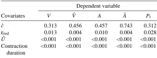
on the pooled data showed that temperature had a significant effect on the variation in the fast-start parameters. Table 4 shows the significance levels for a series of univariate F-tests from the MANCOVA: Uˆ and contraction duration show the strongest correlations with fast-start parameters, and muscle strain εred is also important; however, the body curvature cˆ does not show any significant correlations with the fast-start parameters.
It is interesting to note that the phase of the contraction waves between muscle fibres along the body is a more reliable predictor of fast-start performance than the strain or strain rate used by any one particular fibre. Correlations between an individual muscle’s contractile properties and whole-animal swimming performance should thus be used with caution.
Discussion
Fast-start kinematics
[image:11.609.51.567.85.267.2]Fish fast-starts involve a wave of curvature that travels posteriorly along the spine. This wave is analogous to the wave of curvature during steady swimming (Gray, 1933). As the Table 3. Kinematic parameters describing the first tail-beat of the fast-start
Paracirrhites Serranus Scorpaena Myoxocephalus Notothenia Notothenia
forsteri cabrilla notata scorpius rossii coriiceps
Species (N=23, n=3) (N=37, n=4) (N=40, n=5) (N=15, n=7) (N=25, n=4) (N=31, n=3)
Fast-start temperature 25 20 20 15 1 0
(°C)
Uˆ (s−1) 13.57±1.96 24.45±1.21 17.73±0.91 11.42±1.03 5.17±0.43 4.17±0.23
Vˆmax(s−1) 7.47±0.72 13.15±0.95 10.22±0.55 6.55±0.64 3.16±0.29 2.72±0.13
Aˆmax(s−2) 143.72±14.79 273.81±17.05 223.72±10.96 97.53±6.35 45.91±4.69 39.49±1.82
Aˆmax,tan(s−2) 120.81±14.23 259.75±16.89 193.18±10.86 91.79±6.37 38.81±3.94 34.77±1.95
Piner(W kg−1fish) 13.08±2.95 24.36±2.65 11.78±1.14 5.83±0.82 2.69±0.44 1.51±0.17
L (m) 0.16±0.00 0.12±0.00 0.11±0.00 0.13±0.01 0.25±0.01 0.22±0.00
Vmax(m s−1) 1.18±0.11 1.29±0.14 1.12±0.06 0.83±0.09 0.74±0.05 0.58±0.03
Amax(m s−2) 22.75±2.33 30.74±2.18 24.57±1.20 12.65±0.99 10.62±0.74 8.47±0.40
Amax,tan(m s−2) 19.11±2.24 30.03±2.01 21.13±1.15 11.93±0.94 8.97±0.61 7.46±0.42
Pt(W kg−1muscle) 124.26±29.53 167.18±18.16 104.69±10.14 62.69±8.82 19.44±3.15 16.19±1.82
Mean ±S.E.M. N = number of sequences analysed, n=number of individuals. See symbols list for a full description of the parameters.
Table 4. Univariate F-tests with d.f.=4,114 from the
multivariate analysis of covariance
Dependent variable
Covariates V Vˆ A Aˆ Pt
cˆ 0.313 0.456 0.457 0.743 0.312
εred 0.013 0.004 0.010 0.004 0.028
Uˆ <0.001 <0.001 <0.001 <0.001 <0.001
Contraction <0.001 <0.001 <0.001 <0.001 <0.001 duration
[image:11.609.315.567.615.709.2]body does not flex simultaneously at all positions, it is difficult to categorise a start into discrete stages. Weihs (1973) described fast-starts as consisting of three discrete stages, and Webb (1978) categorised starts into forming initial ‘C’ or ‘S’ shapes. However, body flexion varies with both longitudinal position and time, and so there are no discrete moments when the fish is bent evenly into any particular shape; the starts in the present study achieved a range of body shapes between the classical ‘C’ and ‘S’ shapes. A further problem may be encountered when measuring the tailbeat amplitude for a starting fish which swims on a curved trajectory. Tailbeat amplitude has traditionally been measured as the lateral displacement of the tail from the direction of travel (e.g. Bainbridge, 1958; Videler and Hess, 1984), but swimming on unsteady courses raises uncertainty as to the reference direction. Additionally, yaw of the fish body away from its instantaneous direction will add further discrepancies between a measured tailbeat amplitude and the actual body shape. Quantifying fast-starts by the degree of curvature achieved at the various longitudinal positions has made it possible to compare all starts regardless of the body shapes involved and the course swam.
Fast-start performance is linked strongly to the velocity Uˆ at which the curvature wave travels along the spine (Table 4). The ratio Vˆmax/Uˆ is similar to the slippage ratio Vˆ/Uˆ for steady swimming, which has been used as an indicator of hydrodynamic efficiency (Videler and Hess, 1984). The mean
Vˆmax/Uˆ takes values from 0.54 for P. forsteri to 0.68 for N.
coriiceps. Indeed, there is a significant negative regression
between the slippage ratio Vˆmax/Uˆ and habitat temperature (r2=0.822, P=0.0126), with higher slippage ratios occurring at lower temperatures. Slippage ratios for steady swimming are the ratio of Uˆ to the mean swimming velocity and so would tend to take values greater than this ratio of Vˆmax/Uˆ. Data reviewed by Videler (1993; his Table 6.1) show a slippage ratio of 0.733±0.013 (mean ±S.E.M.) for the steady swimming of 14 species. The slippage ratios during the fast-starts in this study are thus comparable to that in steady swimming, showing an impressive effectiveness of the motion even during the initial moments of the start.
Each fish is able to modulate its fast-start performance by varying Uˆ, as shown for Se. cabrilla in Fig. 10. There has been some debate as to whether fast-starts are controlled by simultaneous muscle activation to all myotomes or by a wave of muscle activation. Jayne and Lauder (1993) measured the onset of EMG activity to be synchronous at different longitudinal positions for the bluegill sunfish Lepomis
macrochirus; however, they measured a posterior propagation
of EMG activity during burst-and-glide swimming in the largemouth bass Micropterus salmoides (Jayne and Lauder, 1995b). If fast-starts were initiated by simultaneous EMG activity in all myotomes, then modulation of Uˆ would not be possible by a change of timing of the activation between myotomes. The slowest mean Uˆ is 4.17 s−1 for N. coriiceps, resulting in a 120 ms delay for the maximum curvature to travel between 0.3L and 0.8L; it is inconceivable that such a delay
can occur as a result of modulatable differences in muscle kinetics along the fish. Indeed, for burst-and-glide swimming, Jayne and Lauder (1995b) found that as the velocity increased the rate of posterior propagation of EMG activity in the deep myomeric muscle also increased. We conclude that the wave of muscle contraction, and hence body curvature, along the fish occurs in part as the result of a posteriorly travelling wave of EMG activity during fast-starts.
Muscle geometry and mechanics
The link between white fibre strain and the adjacent red fibre strain has been treated differently every time it has been considered. Rome et al. (1988) estimated the white fibre strain in carp Cyprinus carpio by using a gearing ratio of 4 (following the reasoning of Alexander, 1969) and estimating red fibre strain using a form of equation 5. Rome and Sosnicki (1991) measured the sarcomere lengths of frozen carp that had gone into rigor. They found that the red fibre strain varied as a function of both the curvature of the spine and the distance of the fibres from the spine. Their white fibre strain varied only as a function of spine curvature. However, these fibres did show significant changes in length between the rigor and post-rigor state. The gearing ratio was found to be 4.25, 2.76 and 1.62 for anterior, middle and posterior regions of the carp, respectively. van Leeuwen et al. (1990) estimated red muscle strain in carp using corrections for fibre orientation. They then calculated white fibre strain by using a gearing ratio of 2. These carp data (van Leeuwen et al.
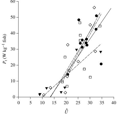
0 5 10 15 20 25 30 35 40
0 10 20 30 40 50 60
U^
Pt
(W kg
[image:12.609.320.549.75.298.2]−1 fish)
1990) were later reanalysed taking a new gearing ratio of 4 (van Leeuwen, 1992).
Fibre orientation changes from a helical geometry in the bulk of the body (Alexander, 1969) to being more parallel to the spine at the caudal peduncle. This change should cause a corresponding change in gearing ratio. In the extreme case, the mean gearing ratio across the fish should approach 2 in the caudal peduncle, and this has been measured in carp (Rome and Sosnicki, 1991). If the gearing ratio does drop to its minimum value of 2 in the caudal myotomes, then the varying muscle geometry along the fish coupled to the specific curvatures employed by these fast-starts would result in the strains and strain rates being similar between the different myotomes (see Fig. 6). Indeed, sonomicrometry measurements have shown the white fibre strain amplitude during fast-starts to be similar at rostral (0.35L) and caudal (0.65L) sites for N. coriiceps (Franklin and Johnston, 1997); similarly, estimates of red muscle strain in carp have shown that, during steady swimming, the change in fish width can exactly compensate for an increasing body curvature to result in similar strains at all positions (van Leeuwen, 1992). If, however, the gearing ratio does not drop to its minimum value of 2, then the strain and strain rate would show a decrease towards the caudal myotomes, resulting in a lower mass-specific power output in this region and a potential for greater force production. The accuracy of the white fibre strain estimates is almost certainly limited by the choice of the gearing ratio. Understanding the functions of different muscles during fast-starts clearly requires information on both muscle structures and geometries along the length of the body as well as detailed kinematic measurements of the body motions.
The fast-starts analysed may not have been at maximum performance and, by definition, they will never have exceeded the maximum possible performance. Therefore, estimates of the mean fast-start power output will necessarily be underestimates of the maximum mechanical power possible from the muscles. Indeed, the estimated muscle-mass-specific total power output of 104.7 W kg−1 for Sc. notata at 20 °C (Table 3) is lower than its measured maximum power available of 142.7 W kg−1(Table 2). This measured muscle power output for Sc. notata is the highest yet measured for a vertebrate muscle and even exceeds the 135 W kg−1measured at 35 °C for the lizard Dipsosaurus dorsalis (Swoap et al. 1993) and the 107.2 W kg−1for the mouse also at 35 °C (James et al. 1995).
Temperature effect on fast-starts
Comparisons of maximum length-specific swimming velocities among the species studied are complicated by differences in body length (Tables 1, 3). Unfortunately, the scaling exponents of Vˆmax are not known for the majority of the species studied. Data in the literature suggest that scaling exponents for Vˆmax vary between species and with the thermal acclimation state of the individual (Temple and Johnston, 1998). It is therefore not advisable to correct Vˆmax to a standard body length using generalised scaling exponents. Nonetheless,
a general trend across all species is that absolute velocities increase whereas length-specific values decrease with increasing fish length (Domenici and Blake, 1997). Despite these opposing scaling relationships between V and Vˆ with L, the data from the present study show an increase in both V and
Vˆ with increasing temperature. There is thus an increase in
fast-start performance due to temperature irrespective of any scaling effects.
Differences in Vˆmax may be expected between distantly related species (Garland and Adolph, 1994). Phylogenetically based comparisons of individuals of identical length would be required to ascertain evolutionary adjustments in Vˆmax between species living at different habitat temperatures (Huey, 1987; Harvey and Pagel, 1991). An interesting observation in the present study was that the Antarctic species N. rossii and N.
coriiceps flexed their bodies with greater curvature than did the
temperate and tropical fish. Comparisons among Notothenidae from Antarctica and from the coast of South America would provide an insight into whether such differences in swimming behaviour were associated with some specific adaptation to low temperatures.
Studies with single skinned muscle fibres (Johnston, 1990) and bundles of live muscle fibres (Johnson and Johnston, 1991) from 20 fish species representing 13 different families show the following patterns: maximum unloaded shortening velocity is positively correlated with mean habitat temperature (see also Fig. 9), whereas maximum force generation falls in the range 160–250 kN m−2. Rates of muscle relaxation are also significantly faster for tropical than for cold-water species at their normal body temperature (Johnson and Johnston, 1991). Power output from a muscle, which is the product of force and shortening velocity, should therefore be correlated with body temperature, a conclusion that holds for work-loop studies in a range of invertebrate and vertebrate species (Stevenson and Josephson, 1990). The relationship between muscle power output and habitat temperature, both measured from work loops and predicted from swimming, for the fast-starts in the present study also fits into this general pattern (Fig. 11). Although quantitative conclusions must await phylogenetically based studies, it would seem that muscle power output decreases at lower temperatures and this in turn limits the fast-start performance of cold-water species.
Conclusions
Fast-starts occur as waves of curvature travelling along the fish body in a manner analogous to steady swimming. Curvature increases in amplitude towards the tail.
The gearing ratio between the red and white muscle strains varies between species for the rostral myotomes.
Increases in median habitat temperature correlate with an increase in the velocity of the wave of curvature along the fish and a decrease in body curvature, peripheral strain and the contraction duration.
the curvature or muscle kinetic properties at any one site along the body. Whole-body performance is thus determined by the concerted action of all the myotomes within the body.
Muscle power output increases with increasing median habitat temperature for the species studied. The initial hydrodynamic power output during the start is proportional to the product of the velocity and acceleration. Therefore, neither velocity nor acceleration is directly proportional to the muscle power output, and thus to the strain rate, during the initial stages of the start. Rather, velocity and acceleration are proportional to the square root of the power. This can be seen from the Q10values for velocity (1.3), acceleration (1.6) and power (2.5).
Fast-start performance is limited by the power available from the muscles; this, in turn, is limited by muscle performance at different temperatures. Antarctic fish muscle delivers lower power output than does temperate and tropical fish muscle, and this results in their having the lowest fast-start performance.
Appendix
Kinematic analyses of fish swimming face the problem of resolving two classes of motion: changes in body shape and changes in body position. Shape changes are caused by the action of the axial muscles stretching and contracting on opposite sides of the body. Information on body shape can thus be used to estimate muscle strain along the body. Changes in
the position of the centre of mass can be used to estimate swimming velocities and accelerations.
When viewed from above, the centre of mass of a straight-stretched fish lies on the spine. During fast-starts, fish can undergo substantial bending, and in such cases the centre of mass moves away from the spine. If the centre of mass is assumed to lie on the spine, then the velocity and acceleration estimates will include a component, due to the bending of the fish, that is not a reflection of the forward motion of the fish.
This Appendix outlines a method that resolves fish motion into its components of changing body shape and body position. The method requires information on the mass distribution along the fish, which is dealt with in the first four sections.
Morphology measurements
Parameters describing fish mass can be determined from a pair of orthogonal images of the fish. Such images are not invasive, are quick to capture and can be taken either from live fish or from those needed fresh and intact for other experiments. For cases where density is homogeneous throughout the body, the distribution of volume mimics the distribution of mass. Thus, the moments of mass and the radii describing these moments are approximated by the moments and radii of the volume distribution.
Longitudinal and planform images only give information about the depth and width of the fish; they will not describe the shape of each transverse section. In this analysis, the fish is assumed to have an elliptical profile in transverse section. As shown by the results, the predicted volume distribution gives a close match to the mass distribution, and this assumption is therefore justified for the species examined here.
Shape parameters
Planform and longitudinal images of freshly killed fish bodies were captured using a JVC TK-1281 video camera, printed with a Sony UP-3000P video printer and then scanned into a Power Macintosh computer. The total length L of the fish was measured using a reference object also captured by the camera. NIH Image version 1.24 software was used to superimpose a grid of 51 equally spaced parallel lines onto the fish outlines with the lines perpendicular to the longitudinal axis of the fish. The coordinates of the intersections of the grid with the fish outlines were digitized and represent the corners of 50 adjacent parallelograms that fit within each image.
0 50 100 150 200
P
(W kg
1 muscle)
0 5 10 15 20 25
Temperature (°C) 1
2 3
4 5
6 7
[image:14.609.54.286.76.267.2]8
Fig. 11. Fish muscle-mass-specific power output as a function of habitat temperature. Open squares are the values of Ptpredicted from the fast-starts in this study. The mean values from all the starts for each species are plotted ± S.E.M. The filled circles are data from work-loop experiments: Notothenia coriiceps (1) (Franklin and Johnston, 1997); Gadhus morhua (2, 4) (Moon et al. 1991; Anderson and Johnston, 1992), respectively; Myoxocephalus scorpius (3, 6, 7) (Altringham and Johnston, 1990; James and Johnston, 1998; G. Temple, personal communication, respectively); Pollachius virens (5) (Altringham et al. 1993); Scorpaena notata (8) (this study).
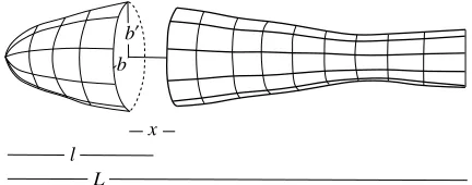
Fig. 12. Each fish segment has width 2b, depth 2b′, thickness x, and has its centre l/L body lengths from the snout.
b
b
x l
[image:14.609.327.543.626.711.2]The body outlines were taken to include the open tail but with the other median and appendicular fins flat on the body; this is all that is required to calculate the mass distribution along the fish. For more detailed hydrodynamic analyses, where the added mass of the fish at all longitudinal positions is required, then the median fins should be extended.
The fish has width 2b and depth 2b′, and each segment (parallelogram) has a length x in the longitudinal direction (Fig. 12). The area sifor each segment is thus approximated
by:
The total area S for the fish is thus:
The longitudinal distance of the centre of each segment from the snout is liand the kth moment of area about the snout is:
For comparative purposes, length and areas can be non-dimensionalised by the fish length L to give:
The non-dimensional radius of the kth moment of area about the snout is thus:
Volume parameters
The volume of each segment vi, as measured from the fish
outlines, is:
and thus the total volume M of the fish is:
The kth moment of the volume about the snout is:
and non-dimensional values for volume and the radius of the
kth moment of area from the snout are:
respectively.
Mass parameters
The body mass m of freshly killed fish was measured on a Mettler PE3000 balance. Fish were frozen, partially thawed and then placed on a square grid with their longitudinal axis parallel to one of the axes of the grid. Approximately 10 transverse sections were cut along the fish; the length of each section was measured with Vernier calipers and the mass mi
measured to the nearest 0.1 g. White myotomal muscle, as judged by its colour, was dissected from each section and weighed separately; i.e. the minor portion of lateral red muscle was excluded from this measurement. The non-dimensional muscle mass mˆmis the proportion of white myotomal muscle to total body mass. A mass loss of 2.0±0.3 % (mean ±S.E.M.) occurred during the cutting procedure. The mass of each section was thus increased by the factor m/∑mito compensate
for this loss. The centre of mass for each section was assumed to lie half-way along the section and was at a distance lifrom
the snout.
The kth moment of mass mkis:
where n is the number of sections cut.
The non-dimensional radius of mkfrom the snout is:
The centre of mass for a straight-stretched fish lies at a radius of lˆ1(m) from the snout. Where mass measurements of the fish segments were not available, they were estimated from the volume distribution. This approximation makes the simplifying assumptions that the densities of the various segments are equal and also that fish bodies are elliptical in cross section. Nonetheless, the linear regression coefficient for
lˆk(m) against lˆk(M) was r2=0.88 (Fig. 4), and so 88 % of the
fish mass distribution can be explained by these simple approximations.
The moment of inertia I about the centre of mass of the fish was determined using a compound pendulum technique. A long hypodermic needle was placed transversely through the midline of a frozen fish, near its tail. The needle, and thus the fish, was balanced on two parallel metal edges, and the fish swung like a pendulum. The moment of inertia for the needle is negligible compared with that of the fish. The fish moment of inertia I is thus given by:
t 2
4π
I = , (A15)
2 rmg
$( )
l m m
mL
k kk
k =
1/
. (A14)
mk m li i n ik = =
∑
1, (A13)
L3
ˆ M
M = and
k k k k ML M M l 1/ ) ( ˆ
= , (A12)
k i i
i
k vl
M
∑
= =50
1
, (A11)
∑
= = 50 1 i i vM . (A10)
x b b
vi= πi i′ , (A9)
$( )
l S S SL
k kk
k =
1/
. (A8)
2 l l ˆ L S S = ,
2 p p ˆ L S S = ,
2 wet wet ˆ L S
S = . (A7)
L l
lˆi = i , (A6)
Sk s li i ik = =
∑
1 50. (A5)
S si i = =
∑
1 50. (A4) planform area , sp,i =2bix, (A1)
longitudinal area , sl,i =2bi′x, (A2)