Online Full Text

(1)

Shengju Sang

FF Abstract—This paper analyzes the buyback contract of a

supply chain including one retailer, one distributor and one supplier in a fuzzy decision making environment. The market demand is characterized as a fuzzy variable. To defuzzify the fuzzy number into a crisp one, the weighted possibilistic mean value method is applied, and the risk attitudes of the supply chain members are also considered. The centralized decision-making model and the buyback contract are proposed, and their optimal solutions are also derived. Finally, the impacts of the retail price, risk basic coefficient, and values of the contract parameters are analyzed for illustrating the results of the proposed fuzzy supply chain models with the help of numerical experiments.

Index Terms—supply chain, risk preference, buyback contract, fuzzy demand

I. 0BINTRODUCTION

OWADAYS, buyback contract has been widely used in practice such as Christmas decorations, seasonal products and in the personal computers industry. In this contract, all firms, which are took part in supply chain, tend to set their order quantities to optimize their total profits of the supply chain system.

In the past ten years, studying the buyback contract with random demand has been investigated by many scholars. For instance, Choi et al. [1] studied the roles of the return policies on the e-marketplace in a two level supply chain. Ding and Chen [2] analyzed a three level supply chain in which the buyback contract was employed to coordinate the chain with one manufacturer, one distributor and one retailer. Chen [3] analyzed the impact of the sharing customer returns information on the buyback contract. Chen and Bell [4] proposed the customer returns policies to coordinate the dual-channel supply chain. Zhao et al. [5] invested the effect of demand uncertainty on the order quantity and wholesale price of the buyback contract, and compared it with the conditions of no buyback policies. Xu et al. [6] proposed a buyback contract for determining the pricing policy, ordering policy and return deadline in a newsboy setting. Some researches also studied the buyback contract in a price-dependent stochastic demand setting, where the demand is a function of retail price in the

Manuscript received April 10, 2016; revised August 15, 2016. This work was supported by the Shandong Provincial Natural Science Foundation, China (No. ZR2015GQ001), and the Project of Shandong Provincial Higher Educational Humanity and Social Science Research Program (No. J15WB04).

Shengju Sang is with the Department of Economics and Management, Heze University, Heze, 274015, China (phone: +86 15853063720; e-mail: [email protected]).

additive or multiplicative model. For instance, Yao et al. [7] analyzed the effects of price-sensitivity factors on the optimal solutions of the buyback contract and the Stackelberg game was employed to solve the models. Gurnani et al. [8] studied the use of the return policies including partial returns, no returns and full returns. Chen and Bell [9] proposed a return policy for coordinating a decentralized supply chain in this setting. Arcelus et al. [10] also studied the buyback policies in this setting, and they mainly concentrated on the risks of demand uncertain. In addition, Ai et al. [11] proposed a full buyback policy when two supply chains competed with each other in an uncertain demand setting. Wu [12] also used a buyback contract to coordinate the competing supply chains, where the vertical integration model and manufacturer’s Stackelberg game were provided to solve the problems. Huang et al. [13] invested a buyback contract for coordinating a chain with one supplier and many competing retailers with a secondary market.

The risk attitudes of the actors were also considered in the buyback contract with random demand. Choi et al. [14] discussed the profit and risk sharing problem by using the mean-variance method under a returns policy. Hsieh and Lu [15] proposed a buyback contract for coordinating a supply chain with one manufacturer and two risk-averse retailers in a random demand environment. Yoo [16] also discussed the risk preference problem in a buyback contract, where they considered the supplier’s two different risk attitudes including risk averse and risk neutral.

Recently, fuzzy set theory has been applied to solve the supply chain coordination mechanism problems, where the demands are defined as fuzzy variables. Yu and Jin [17] adopt signed distance method to study the buyback contract, where they considered the demand and the retail price as the triangular fuzzy numbers. Yu et al. [18] also studied the fuzzy newsboy model with return policies in a price-dependent demand environment. Chang and Yeh [19] analyzed the buyback policies of the decentralized and centralized supply chains with fuzzy demand. Sang [20] studied the buyback contract with multiple competing retailers in a fuzzy demand environment. Zhang et al. [21] used the crisp possibilistic mean method to study a two level return contract in a fuzzy random demand environment. Yano et al. [22] proposed the multi-objective fuzzy random linear programming problems based on coefficients of variation. Sang [23] studied a revenue sharing contract with fuzzy demand in a three-echelon supply chain. Yang et al. [24] developed a fuzzy three-echelon inventory model with defective products and rework under credit period.

The works mentioned above studied the fuzzy buyback

Buyback Contract with Fuzzy Demand and Risk

Preference in a Three Level Supply Chain

N

IAENG International Journal of Applied Mathematics, 46:4, IJAM_46_4_16

(2)

contract in a two level supply chain and considered the actors as risk neutral. In this paper, we extend their works to a three level supply chain, and the risk attitudes of the actors are also considered. Furthermore, we analyze the impact of the retail price, the risk basic coefficient, and the values of contract parameters on the buyback policies.

The paper is organized as follows. In Section II, we briefly described the problem and the notations that will be used in the following sections. In Sections III, we developed the centralized decision-making system and the buyback contract. In Section IV, three numerical examples are given to illustrate the solutions for proposed models. Section V summarizes the work.

II. 1BPROBLEM DESCRIPTIONS

In this paper, we consider a three level supply chain which consists of a supplier, a distributor and a retailer (see Figure I).

The following notations are used in the models: p: unit fixed retail price of the market;

1

w: unit wholesale price offered by the supplier;

2

w : unit wholesale price offered by the distributor;

1

b : unit return price of unsold product offered by the supplier;

2

b : unit return price of unsold product offered by the distributor;

s: unit salvage value of unsold product;

1

c: unit cost incurred to the supplier;

2

c : unit cost incurred to the distributor;

3

c : unit cost incurred to the retailer; q: The order quantity.

Letc= + +c1 c2 c3be the unit cost incurred to the supply

chain system.

For some high-tech products such as PC, it is difficult to predict their accurate demands duce to lack of historical data. In this situation, the demand is usually estimated by the decision maker. In this paper, we considered the demand estimated by the decision maker as a positive trapezoidal fuzzy number withD% =

(

d d d d₁, ₂, ₃, ₄

)

. It means that most possible value of the demand is betweend₂andd₃, the lower bound and upper bound of the demand ared1andd4,

respectively. The membership function of the fuzzy demandμ_D_%

( )

x is stated as

( )

1 2

2 3

3 4

, ,

1, ,

, ,

0, .

D

L x d x d

d x d

x

R x d x d

otherwise

μ

≤ < ⎧

⎪

≤ ≤ ⎪

= ⎨

< ≤ ⎪

⎪ ⎩

% (1)

Where, the left membership function

( )

1 2 1

x d L x

d d

− =

− is

increasing with d1≤ <x d2 , and the right membership

function

( )

4 4 3

d x

R x

d d

− =

− is decreasing withd3≤ <x d4.

To convert the fuzzy number into a crisp one, Carlsson and Prade [25] proposed a ranking method, namely the weighted possibilistic mean value method as

(

) ( )

( )

(

)

1

1 1

0 1 d

M D⎡ ⎤ =_{⎣ ⎦}%

∫

−T L− λ +TR− λ λ (2) where_⎣⎡L−1

( )

λ ,R−1

( )

λ ⎤_⎦ is theλ level set of the fuzzy numberD% , and T

(

0< <T 1

)

reflects the risk attitude of the decision maker. When 1

2

T = , the attitude of the decision maker is risk neutral, When 1

2

T < , the attitude of the decision maker is pessimistic, the lower the value ofT, the more risk adverse of the decision maker, and when 1

2

T > , the attitude of the decision maker is optimistic, the higher the value ofT, the more risk preference of the decision maker.

To avoid trivial cases, the following assumptions should be met:

2 1

s+b <b,w1+c2 <w2, ands+ <bi wi,i=1, 2.

III. 2BMODELS AND SOLUTION APPROACHES

In this section, we consider a centralized decision-making system and a buyback contract of the supplier, the distributor and the retailer in a fuzzy demand environment. A. Centralized decision-making system

In a centralized decision-making system, the supplier, the distributor and the retailer cooperate with each other, and their total fuzzy profit can be described as

{ }

{

}

min , max , 0

SC p q D s q D cq

Π =% % + − % − (3)

The problem of the supply chain system is to seek the optimal order quantity to maximum the weighted possibilistic mean value of the supply chain’s fuzzy profit

( )

SC

M Π% , which is given by

( )

(

{ }

{

}

)

Max_qM Π%_SC =M pmin q D, % +smax q D− %,0 −cq s.t .d1≤ ≤q d4 (4)

Since the demandD% =

(

d d d d1, 2, 3, 4

)

is a fuzzy variable,

then it shows that the optimal order quantity has three conditions, namelyq∈

[

d d1, 2

)

,q∈

[

d d2, 3

]

andq∈

(

d d3, 4

]

.

Condition 1: q∈

[

d d₁, ₂

)

In this condition, the α cut set of min

{ }

q D, % and

{

}

max q−D%, 0 are

{ }

(

)

[ ]

1

( )

, , 0 ,

min ,

, , 1.

L q L q

q D

q q L q

α

α α

α −

⎧⎡ ⎤ < ≤

⎪⎣ ⎦

= ⎨

< < ⎪⎩

%

{

}

(

)

[ ]

1

( )

, , 0 ,

max , 0

, , 1.

q L q L q

q D

q q L q

α

λ α

α −

⎧⎡ − ⎤ < ≤

⎪⎣ ⎦

− _{= ⎨}

< < ⎪⎩

%

Then, theλlevel set of Π%SCis w2

w1

b1 b2

p

FIGURE I

BUYBACK CONTRACT IN A THREE LEVEL SUPPLY CHAIN Distributo

r

Retailer Customer Supplier

IAENG International Journal of Applied Mathematics, 46:4, IJAM_46_4_16

(3)

( )

(

( )

)

( )

[

]

( )

1 1

, ,

0 ,

, , 1.

SC

pL s q L cq pq cq

L q

pq cq pq cq L q

λ

λ λ

− −

⎧⎡_⎣ + − − − ⎤_⎦ ⎪⎪

Π =_⎨ < ≤ ⎪ ₋ ₋ _{< <} ⎪⎩

%

Using (2), the weighted possibilistic mean value of the supply chain’s fuzzy profitM

( )

Π%SC is

( )

(

)

(

1

( )

(

1

( )

)

0 1

L q

SC

M Π% =

∫

−T pL− λ +s q L− − λ −cq +T pq

(

−cq

)

dλ

(

)(

)

(

)

(

)

( )

1

1 d

L q T pq cq T pq cq λ

+

∫

− − + −

(

)(

)

( )

(

( )

)

1 0

1 L q d

pq T p s q L− λ λ cq

= − − −

∫

− − (5)

The first order condition is

( )

(

)(

) ( )

d

1 d

SC

M

p T p s L q c

q

Π

= − − − −

%

The second order condition is

( )

(

)(

) ( )

2

' 2

d

1 d

SC

M

T p s L q q

Π

= − − −

%

Since p>s, 0< <T 1, and L q

( )

is increasing with

( )

'

0

L q > , therefore, M

( )

Π%SC is concave with respect

toq. Hence, the first order conditiond

( )

0 d

SC

M

q

Π =

%

gives

( )

*

(

)(

)

1

p c L q

T p s

− =

− − (6)

If

(

1

)(

)

1

p c T p s

− _<

− − , namely,T p

(

− < −s

)

c s, then

(

)(

)

* 1

1

p c

q L

T p s

− ⎛ − ⎞

= ⎜_⎜ ₋ ₋ ⎟_⎟

⎝ ⎠ (7)

The optimal weighted possibilistic mean value of the supply chain’s fuzzy profitM

( )

Π%_SC *in this condition is

( )

(

)(

)

( )*

( )

* ₁

0

1 L q d

SC

M Π% = −T p−s

∫

L− λ λ (8) Condition 2: q∈

[

d d2, 3

]

{ }

q D, % and

{

}

max q−D%, 0 are

{ }

(

)

1

( )

min q D, L ,q

α α

−

⎡ ⎤ = ⎣ ⎦

%

{

}

(

_max _q _D_{, 0}

)

_q _L1

( )

_,_q

α α

−

⎡ ⎤

− % =_⎣ − _⎦

Then, theλlevel set of Π%SCis

( )

1

( )

(

1

( )

)

_, SC _λ pL λ s q L λ cq pq cq

− −

⎡ ⎤

Π% =_⎣ + − − − _⎦

( )

Π%SC is

( )

1

(

)

(

( )

(

( )

)

1 1

0 1

SC

M Π% =

∫

−T pL− λ +s q−L− λ −cq

(

)

d

T pq cq λ

+ −

(

)

(

T p s s q

)

cq

= − + −

(

)(

)

1 ₁

( )

0

1 T p s L− λ λd

+ − −

∫

(9) The first order condition is

( )

(

)

d

SC

M

T p s s c q

Π

= − + −

%

When T p s

(

− > −

)

c s , M

( )

Π%_SC is increasing with respect toq , and gets its optimal value atd3, when

(

)

T p− < −s c s, M

( )

Π%SC is decreasing with respect toq,

and gets its optimal value atd2, and when T p s

(

− = −

)

c s,

( )

SC

M Π% obtains its optimal value for any *

[

]

2, 3

q ∈ d d . In this condition, we can conclude that

{ }

(

)

(

)

{ }

(

)

2 *

2 3 3

, ,

[ , ], ,

, .

d T p s c s

q d d T p s c s

d T p s c s

− < − ⎧

⎪

∈⎨ − = − ⎪ _{− > −} ⎩

(10)

Condition 3: q∈

(

d d₃, ₄

]

{ }

q D, % and

{

}

max q−D%, 0 are

{ }

(

)

11

( )

1

( )

, , 0 ,

min ,

, , 1.

L q R q

q D

L R R q

α

α α

α α α

−

− −

⎧⎡ ⎤ < ≤ ⎪⎣ ⎦

= ⎨

⎡ ⎤ < <

⎪⎣ ⎦

⎩

%

{

}

(

)

11

( )

1

( )

, , 0 ,

max ,0

, , 1.

q L q R q

q D

q L q R R q

α

α α

α α α

−

− −

⎧⎡ − ⎤ < ≤

⎪⎣ ⎦

− _{= ⎨}

⎡ − − ⎤ < <

⎪⎣ ⎦

⎩

%

Then, theλlevel set of Π%SCis

( )

(

( )

)

( )

(

( )

)

( )

(

( )

)

( )

1 1

, , 0 ,

,

, 1.

SC

pL s q L cq pq cq R q

pL s q L cq

pR s q R cq R q

λ

λ λ λ

λ λ

λ λ λ

− −

⎧⎡_⎣ + − − − ⎤_⎦ < ≤ ⎪

⎪⎡

Π =_⎨⎣ + − −

⎪

⎤

⎪ + − − _⎦ < <

⎩

%

( )

Π%SC is

( )

(

)

(

1

( )

(

1

( )

)

0 1

R q SC

M Π% =

∫

−T pL− λ +s q−L− λ −cq

(

)

d

T pq cq λ

+ −

(

)

(

( )

(

( )

)

(

( )

1 ₁ ₁

1

R q T pL λ s q L λ cq

− −

+

∫

− + − −

( )

(

( )

)

(

1 1

)

_d

T pR− λ s q R− λ cq λ

+ + − −

(

)

(

1 ₁

( )

)

( ) d

R q

T p s R− λ λ qR q sq cq

= −

∫

+ + −

(

)(

)

1

( )

1 0

1 T p s L− λ λd

+ − −

∫

( )

(

) ( )

d

SC

M

T p s R q s c q

Π

= − + −

%

IAENG International Journal of Applied Mathematics, 46:4, IJAM_46_4_16

(4)

( )

(

) ( )

2

' 2

d

SC

M

T p s R q q

Π

= −

%

Since p>s , T >0 , and R q

( )

is decreasing with

( )

'

0

R q < , therefore, in this condition M

( )

Π%SC is

concave with respect toq. Hence, the first order condition

( )

d

0 d

SC

M

q

Π =

%

gives

( )

*

(

c s

)

R q

T p s

− =

− (12)

If

(

c s

)

1 T p s

− <

− , namely,T p s

(

− > −

)

c s, then

(

)

* 1 c s

q R

T p s

− ⎛ − ⎞

= ⎜_⎜ ⎟_⎟ −

⎝ ⎠ (13)

Therefore, in this condition,M

( )

Π%SC *is

( )

(

)

(

*

( )

(

)

( )

)

1 1

* ₁ ₁

( ) d 1 0 d

SC _{R q}

M Π% = p s T−

∫

R− λ λ+ −T

∫

L− λ λ (14)

Combining the three conditions, whenT p s

(

− < −

)

c s, we haveM

(

Π%SC

( )

q*

)

≥M

(

Π%SC

( )

d2

)

, and whenT p s

(

− > −

)

c s,

we have

(

( )

)

(

( )

*

)

3

SC SC

M Π% d ≤M Π% q .

From the above discussions, we can have the following theorem.

Theorem 1. The optimalorder quantity *

q is

(

)(

)

(

)

(

)

(

)

(

)

1 *

2 3 1

, ,

1

[ , ], ,

, .

p c

L T p s c s

T p s

q d d T p s c s

c s

R T p s c s

T p s

−

⎧ ⎛ − ⎞

− < − ⎪ ⎜_⎜ ₋ ₋ ⎟_⎟

⎪ ⎝ ⎠ ⎪

=_⎨ − = −

⎪ _⎛ _⎞ −

⎪ _⎜ _⎟ _{− > −} ⎪ ⎜ ₋ ⎟

⎝ ⎠ ⎩

(15)

Remark 1. Ifd2=d3, then the fuzzy demand degenerates

to a triangular fuzzy number, and the result in Theorem 1 degenerates to

(

)(

)

(

)

(

)

(

)

1 *

1

, ,

1

, .

p c

L T p s c s

T p s q

c s

R T p s c s

T p s

−

⎧ ⎛ − ⎞

− < − ⎪ ⎜_⎜ ⎟_⎟

− − ⎪ ⎝ ⎠ = ⎨

⎛ ₋ ⎞

⎪ _{− > −} ⎜ ⎟

⎪ ⎜ ₋ ⎟ ⎝ ⎠ ⎩

(16)

The optimal weighted possibilistic mean value of the supply chain’s fuzzy profit M

( )

Π%SC *is

( )

(

)(

)

( )( )

( )

(

)

(

)(

)

( )

(

)

(

)

( )

(

)

( )

(

)

1 1 0 1

1

* 0

1 ₁ 1 ₁

0

1 d , ,

d 1 d ,

.

p c T p s

SC

c s T p s

T p s L T p s c s

M

p s T R T L

T p s c s

λ λ

λ λ λ λ

− − − −

−

− −

⎧

− − − < − ⎪

⎪

⎪ − − − = − ⎪

Π _{= ⎨}

⎛ ⎞

⎪ − ⎜ + − ⎟

⎪ _⎜ _⎟

⎝ ⎠

⎪

⎪ _{− > −}

⎩

∫

%

B. Buyback contract

With a buyback contract, the supplier offers return policy to the distributor, and the distributor offers return policy to the retailer for the unsold products at the end of a single selling season. Therefore, the fuzzy profit for the retailer is

{ }

2

{

}

(

2 3

)

min , max , 0

R p q D b q D w c q

Π =% % + − % − + (17)

The fuzzy profit for the distributor is

(

2 1 2

)

1max

{

,0

}

2max

{

,0

}

D w w c q b q D b q D

Π =% − − + −% − −% (18)

The fuzzy profit for the supplier is

(

1 1

)

max

{

, 0

}

1max

{

, 0

}

S w c q s q D b q D

Π =% − + − % − − % (19)

The problems of the retailer and the distributor are to seek their optimal order quantities to maximum their weighted possibilistic mean value of the fuzzy profit

( )

R

M Π% andM

( )

Π%_D , respectively

( )

(

{ }

2

{

}

Max_qM Π =%_R M pmin q D, % +b max q−D%, 0

(

w2 c q3

)

− +

1 4

s.t .d ≤ ≤q d (20) and

( )

(

2 1 2

)

1

{

}

Max_qM Π =%_D M w − −w c q b+ max q D− %,0

{

}

)

2max ,0

b q D

− − %

1 4

s.t .d ≤ ≤q d (21) Theorem 2. The optimal strategies

(

* *

)

2 , 2

b w and

(

* *

)

1, 1

b w

in the buyback contract satisfy the following equations

(

1 2

) (

3

)

* *

2 2

p c c p c s

p s

b w

p c p c

+ − − −

= −

− − (22)

(

)

1 2 3

* *

1 1

pc p c c s p s

b w

p c p c

− − − −

= −

− − (23)

Proof: Three conditions are considered as follows. Condition 1: q∈

[

d d₁, ₂

)

Like previous conditions, the weighted possibilistic mean value of the retailer’s fuzzy profitM

( )

Π%_R is

( )

(

)(

)

( )

(

₁

( )

)

2 ₀

1 L q d

R

M Π =% pq− −T p b−

∫

q−L− λ λ

−

(

w2+c q3

)

(24)

The first order condition is

( )

(

)(

) ( )

2 2 3

d

1 d

R

M

p T p b L q w c

q

Π

= − − − − −

%

( )

(

)(

) ( )

2

' 2 2

d

1 d

R

M

T p b L q q

Π

= − − −

%

Since p>b₂ ,0< <T 1 , and L q

( )

is increasing with

( )

' ₀

L q > , therefore, in this condition, M

( )

Π%_R is concave with respect to q . Hence, the first order condition

IAENG International Journal of Applied Mathematics, 46:4, IJAM_46_4_16

(5)

( )

d

0 d

R

M

q

Π =

%

gives

( )

**

(

)(

2 3

)

2

1

p w c

L q

T p b

− − =

− − (25)

In order to obtain coordination of this supply chain,

** *

q =q must be hold. That is

(

1

)(

2 32

) (

1

)(

)

p w c p c

T p b T p s

− − ₌ −

− − − − (26)

Solving (26), we have

(

1 2

) (

3

)

* *

2 2

p c c p c s

p s

b w

p c p c

+ − − −

= −

− −

The weighted possibilistic mean value of the distributor’s fuzzy profitM

( )

Π%D in this condition is

( )

(

) (

)(

)

( )

(

₁

( )

)

2 1 2 1 2 1 ₀ d

L q D

M Π =% w − −w c q− −T b −b

∫

q L− − λ λ(27) The first order condition is

( )

(

)(

) ( )

2 1 2 2 1

d

1 d

D

M

w w c T b b L q

q

Π

= − − − − −

%

( )

(

)(

) ( )

2

' 2 1 2

d

1 d

D

M

T b b L q q

Π

= − − −

%

Sinceb₂ >b₁, 0< <T 1, and L q

( )

is increasing with

( )

'

0

L q > , therefore, in this condition, M

( )

Π%_D is concave with respect to q . Hence, the first order condition

( )

d

0 d

D

M

q

Π =

%

gives

( )

**

(

2

)(

1 2

)

2 1

1

w w c

L q

T b b

− − =

− − (28)

* **

(

1

)(

) (

1 2

)(

12 21

) (

1

)(

2 32

)

p w c

w w c

p c

T p s T b b T p b

− −

− ₌ ₌

− − − − − −

(

1 1

)(

2 1

)

3

p w c c

T p b

− − −

=

− − (29)

(

)

1 2 3

* *

1 1

pc p c c s p s

b w

p c p c

− − − −

= −

− −

Condition 2: q∈

[

d d2, 3

]

( )

Π%_R is

( )

(

)

(

)(

)

1 ₁

( )

2 2 1 2 ₀ d

R

M Π =% T p b− +b q+ −T p b−

∫

L− λ λ

(

w2 c q3

)

− + (30) The first order condition is

( )

(

)

2 2 2 3

d

R

M

T p b b w c

q

Π

= − + − −

%

WhenT p b

(

− ₂

)

>w₂+ −c₃ b₂, M

( )

Π%_R is increasing with respect to q , and gets its optimal value at d₃ , whenT p b

(

− 2

)

<w2+ −c3 b2, M

( )

Π%R is decreasing with

respect to q , and gets its optimal value at d2 , and

whenT p b

(

− 2

)

=w2+ −c3 b2, M

( )

Π%R obtains its optimal

value for any **

[

]

2, 3

q ∈ d d .

In order to obtain coordination of this supply chain,q**=q*must be hold.

That is

(

)

(

)

2 3 2 2

w c b c s

T p b T p s

+ − −

=

− − (31)

(

1 2

) (

3

)

* *

2 2

p c c p c s

p s

b w

p c p c

+ − − −

= −

− −

( )

D

(

2 1 2

) (

1

)(

2 1

)

M Π =% w −w −c q− −T b −b q

(

)(

)

1

( )

1 2 1 ₀

1 T b b L− λ λd

+ − −

∫

( )

(

)

2 1 2 1 2 1 2

d

D

M

T b b w w c b b

q

Π

= − + − − + −

%

WhenT b b

(

₂− > − + + −₁

)

w w c₁ ₂ ₂ b₂ b₁, M

( )

Π%_D is increasing with respect to q , and gets its optimal value atd₃, when T b

(

2−b1

)

<w1−w2+ + −c2 b2 b1 , M

( )

Π%D is

decreasing with respect toq, and gets its optimal value atd₂, and whenT b

(

2−b1

)

= − + + −w1 w2 c2 b2 b1, M

( )

Π%D obtains its

optimal value for any **

[

]

2, 3

q ∈ d d .

* **

(

)

1 2

(

22 1

)

2 1 2

(

3 2

)

2

w c b

w w c b b

c s

T p s T b b T p b

+ − − + + −

−

= =

− − −

(

)

1 1 2 3 1

w b c c

T p b

− + + =

− (33)

(

)

1 2 3

* *

1 1

pc p c c s p s

b w

p c p c

− − − −

= −

− −

Condition 3: q∈

(

d d3, 4

]

( )

Π%R is

IAENG International Journal of Applied Mathematics, 46:4, IJAM_46_4_16

(6)

( )

(

)

(

1 ₁

( )

)

(

)

2 _{( )} d 2 2 3

R _{R q}

M Π =% T p b−

∫

R− λ λ+qR q +b q− w +c q

(

)(

)

1

( )

1 2

0

1 T p b L− λ λd

+ − −

∫

( )

(

) ( )

1 2 2 3

d

R

M

T p b R q b w c q

Π

= − + − −

%

( )

(

) ( )

2

' 2 2

d

R

M

T p b R q q

Π

= −

%

Since p>b2 , T >0 and R q

( )

is decreasing with

( )

'

0

R q < , therefore, in this condition,M

( )

Π%R is concave

with respect to q . Hence, the first order condition

( )

d

0 d

R

M

q

Π =

%

gives

( )

** 2

(

3

)

2 1

w c b

R q

T p b

+ − =

−

In order to obtain coordination of this supply chain,q**=q*must be hold.

That is

(

)

(

)

2 3 2 1

w c b c s

T p b T p s

+ − ₌ −

− − (35)

(

1 2

) (

3

)

* *

2 2

p c c p c s

p s

b w

p c p c

+ − − −

= −

− −

( )

D

(

2 1 2

) (

2 1

)

(

2 1

)

( )

M Π% = w −w −c q− b −b q T b+ −b qR q

(

)

1

( )

1 2 1 _{R q}_{( )} d

T b b R− λ λ

+ −

∫

(

)(

)

1

( )

1 2 1 ₀

1 T b b L− λ λd

+ − −

∫

( )

(

) ( )

2 1 2 1 2 2 1

d

D

M

T b b R q w w c b b

q

Π

= − + − − − +

%

( )

(

) ( )

2

' 2 1 2

d

D

M

T b b R q q

Π

= −

%

Since b₂>b₁ ,T >0 , and R q

( )

is decreasing with

( )

'

0

R q < , therefore, in this condition,M

( )

Π%_D is concave with respect to q . Hence, the first order condition

( )

d

0 d

D

M

q

Π =

%

gives

( )

** 1 2

(

2

)

2 1 2 1

w w c b b

R q

T b b

− + + − =

−

* **

(

)

1 2

(

22 1

)

2 1 2

(

3 1

)

2 1

(

2 32

)

1

w c b w c c b

w w c b b

c s

T p s T b b T p b T p b

+ − + + −

− + + −

− ₌ ₌ ₌

− − − − (37)

(

)

1 2 3

* *

1 1

pc p c c s p s

b w

p c p c

− − − −

= −

− −

The proof of Theorem 2 is completed. Theorem 3. For0<λ₁<1and 3

2 1

s c c s λ

+

< <

− , the set of

buyback contract strategies

(

* *

)

2 , 2

b w and

(

* *

)

1, 1

b w satisfy

(

)

*

2 2

b = −p λ p−s (38)

(

)

*

2 3 2

w = − −p c λ p c− (39)

(

)(

)

*

1 1 1 1 2

b = + −s λ −λ p−s (40)

(

)(

)

*

1 1 1 1 1 2

w = + −c λ −λ p c− (41) Proof: Substituting *

2

w in (39) into (22), we have

(

)

*

2 2

b = −p λ p−s Sinceb₂+ <s w₂, we have 3

2

s c c s

λ > + − .

Substituting * 1

w in (41) into (23), we have

(

)(

)

*

1 1 1 1 2

b = + −s λ −λ p−s Forλ₁>0, b₁+ <s w₁ands+b₂<b₁. The proof of Theorem 3 is completed. Theorem 4. For0<λ1<1and

3

2 1

s c c s λ

+

< <

− , the supply

chain actors obtain their optimal weighted possibilistic mean value of fuzzy profits at

(

* *

)

2 , 2

b w and

(

* *

)

1, 1

b w as follows

( )

*

( )

*

2

R SC

M Π% =λ M Π% (42)

( )

*

(

)

( )

*

1 1 2

D SC

M Π% =λ −λ M Π% (43)

( )

*

(

)(

)

( )

*

1 2

1 1

S SC

M Π% = −λ −λ M Π% (44) Proof: Condition 1:

Substituting * 2

b , * 2

w and _{L q}

( )

* _{in (6) into (24), we can}

get the optimal weighted possibilistic mean value of the retailer’s fuzzy profitM

( )

Π%_R *as

( )

*

(

)(

)

( )( ) ₁

( )

1

2 1 ₀ d

p c T p s R

M λ T p s L λ λ

− − − −

Π% = − −

∫

( )

* 2M SC

λ

= Π% Substituting *

2

b , * 2

w , * 1

b , * 1

w and_{L q}

( )

*

into (27), we can get the optimal weighted possibilistic mean value of the distributor’s fuzzy profit M

( )

Π%_D *as

( )

*

(

)(

)

( )( ) ₁

( )

1

1 1 2 1 ₀ d

p c T p s D

M λ λ T p s L λ λ

− − − −

Π% = − − −

∫

(

)

( )

*

1 1 2 M SC

λ λ

= − Π%

Then, the optimal weighted possibilistic mean value of the supplier’s fuzzy profitM

( )

Π%S *is given as

IAENG International Journal of Applied Mathematics, 46:4, IJAM_46_4_16

(7)

( )

*

( )

*

( )

*

( )

*

S SC R D

M Π% =M Π% −M Π% −M Π%

(

)(

)

( )

*

1 2

1 λ 1 λ M _SC

= − − Π% Condition 2:

Substituting * 2

b , * 2

w and T p s

(

− = −

)

c sinto (30), we can get the optimal weighted possibilistic mean value of the retailer’s fuzzy profitM

( )

Π%R *as

( )

*

(

)(

)

1 ₁

( )

2 1 ₀ d

R

M Π% =λ −T p−s

∫

L− λ λ =λ₂M

( )

Π%_SC * Substituting *

2

b , * 2

w , * 1

b , * 1

w andT p s

(

− = −

)

c s into (32), we can get the optimal weighted possibilistic mean value of the distributor’s fuzzy profitM

( )

Π%_D *as

( )

*

(

)(

)

1 ₁

( )

1 1 2 1 ₀ d

D

M Π% =λ −λ −T p−s

∫

L− λ λ

(

)

( )

*

1 1 2 M SC

λ λ

= − Π%

( )

Π%_S * in this condition is given as

( )

*

( )

*

( )

*

( )

*

S SC R D

M Π% =M Π% −M Π% −M Π%

(

)(

)

( )

*

1 2

1 λ 1 λ M _SC

= − − Π% Condition 3:

Substituting * 2

b , * 2

w and_{R q}

( )

* _{in (12) into (34), we can}

get the optimal weighted possibilistic mean value of the retailer’s fuzzy profitM

( )

Π%R *as

( )

(

)

( )

(

)

( )

1 1

* ₁ ₁

2 c s d 1 ₀ d

R

T p s

M λ p s T − R− λ λ T L− λ λ

−

⎛ ⎞

Π = − ⎜_⎜ + − ⎟_⎟

⎝

∫

⎠

%

=λ₂M

( )

Π%_SC * Substituting *

2

b , * 2

w , * 1

b , * 1

w and_{R q}

( )

*

into (36), we can get the optimal weighted possibilistic mean value of the distributor’s fuzzy profit M

( )

Π%_D *as

( )

(

)(

)

( )

(

)

( )

1 1

* ₁ ₁

11 2 c s d 1 ₀ d

D

T p s

M λ λ p s T − R− λ λ T L− λ λ

−

⎛ ⎞

Π = − − ⎜_⎜ + − ⎟_⎟

⎝

∫

⎠

%

=λ1

(

1−λ2

)

M

( )

Π%SC *

( )

Π%_S * in this condition is given as

( )

*

( )

*

( )

*

( )

*

S SC R D

M Π% =M Π% −M Π% −M Π%

(

)(

)

( )

*

1 2

1 λ 1 λ M _SC

= − − Π% The proof of Theorem 4 is completed.

IV. 3BNUMERICAL EXAMPLES

In this section, we provide three numerical examples to show the effects of retail price p , the risk basic coefficientT, and the values of parametersλ1andλ2on the

optimal policies. Letc1=50,c2=15,c3=10and s=15. We

further assume that the most possible value of the market demand is between 200 and 300, the demand is no less than 100 and no more than 400, that isD% =

(

100, 200, 300, 400

)

.

From Theorem 4, we have0.42<λ₂ <1. Discussion A

In this subsection, we discuss the effect of retail pricepon the optimal policies in the buyback contract. Let

1 0.40

[image:7.595.304.551.208.484.2]

λ = and λ₂ =0.50 . The optimal solutions in the buyback contract are given in Tables I and II.

TABLE I

THE OPTIMAL PRICES IN BUYBACK CONTRACT WITH DIFFERENT p

T p *

q b1*

* 1

w *

2

b *

2 w

0.40 155 195 57.0 74.0 85.0 105.0

160 198 58.5 75.5 87.5 107.5

165 [200,300] 60.0 77.0 90.0 110.0

170 303 61.5 78.5 92.5 112.5

175 306 63.0 80.0 95.0 115.0

0.50 125 191 48.0 65.0 70.0 90.0

130 196 49.5 66.5 72.5 92.5

135 [200,300] 51.0 68.0 75.0 95.0

140 304 52.5 69.5 77.5 97.5

145 308 54.0 71.0 80.0 100.0

0.60 105 183 42.0 59.0 60.0 80.0

110 192 43.5 60.5 62.5 83.5

115 [200,300] 45.0 62.0 65.0 85.0

120 305 46.5 63.5 67.5 87.5

125 309 48.0 65.0 70.0 90.0

TABLE II

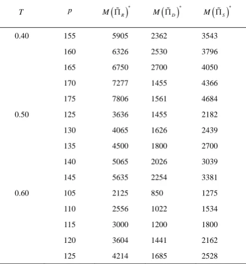
THE OPTIMAL PROFITS OF THE MEMBERS WITH DIFFERENT p

T p M

( )

Π%R *

( )

*

D

M Π% M

( )

Π%S *

0.40 155 5905 2362 3543

160 6326 2530 3796

165 6750 2700 4050

170 7277 1455 4366

175 7806 1561 4684

0.50 125 3636 1455 2182

130 4065 1626 2439

135 4500 1800 2700

140 5065 2026 3039

145 5635 2254 3381

0.60 105 2125 850 1275

110 2556 1022 1534

115 3000 1200 1800

120 3604 1441 2162

125 4214 1685 2528

IAENG International Journal of Applied Mathematics, 46:4, IJAM_46_4_16

[image:7.595.306.551.508.770.2]

(8)

From Tables I and II, we can see that: (1) The optimal order quantity_q*

increases as the retail price pincreases. Especially, in this numerical example, when

( ) (

T p, = 0.40,165

)

,

( ) (

T p, =0.50,135

)

and

( ) (

T p, =0.40,115

)

, the optimal order quantityq*can be any values between 200 and 300.

(2) Increasing retail price

p

will increase the wholesale prices *

1

w and * 2

w , the return prices * 1

b and * 2

b , and the optimal weighted possibilistic mean value of the supply chain actor’s fuzzy profit. It indicates that an increase in retail price results in an increase in order quantity. This results in an increase in the supply chain actor’s profit.

DiscussionB

In this subsection, we discuss the effect of the risk basic coefficientTon the optimal policies in the buyback contract. Letp=135,λ₁=0.40 andλ₂ =0.50. We can have *

1 51

b = ,

* 1 68

w = , * 2 75

b = and * 2 95

w = . The other optimal solutions in the buyback contract are given in Table III.

TABLE III

THE OPTIMAL SOLUTIONS IN BUYBACK CONTRACT WITH DIFFERENT T

T *

q M

( )

Π%R *

( )

*

D

M Π% M

( )

Π%S *

0.30 171 4071 1629 2443

0.35 177 4154 1662 2492

0.40 183 4250 1700 2550

0.45 191 4364 1745 2618

0.50 [200,300] 4500 1800 2700

0.55 309 4964 1985 2978

0.60 317 5450 2180 3270

0.65 323 5954 2382 3572

0.70 329 6471 2589 3883

We can see that:

(3) The optimal order quantity *

q increases as the risk basic coefficientTincreases, and can be any values between 200 and 300, whenT=0.50in this case.

(4) The change of the risk basic coefficientTwill not impact on the wholesale prices *

1

w and * 2

w , and the return prices *

1

b and * 2

b .

(5) When the risk basic coefficientT increases, the optimal weighted possibilistic mean values of the fuzzy profits for all actors will increase. This is because the risk basic coefficientTreflects the risk attitude of the supply chain actors. The more responsibility of risk the more weighted possibilistic mean values of the fuzzy profits they can obtain.

Discussion C

In this subsection, we discuss the effects of the values of parametersλ1andλ2on the optimal policies in the buyback

[image:8.595.304.548.172.418.2]

contract. Letp=135and T=0.40. The optimal solutions in the buyback contract are given in Tables IV and V.

TABLE IV

THE OPTIMAL PRICES IN BUYBACK CONTRACT WITH DIFFERENTλ1ANDλ2

(λ λ1, 2)

*

q b1*

* 1

w *

2

b *

2 w

(0.40, 0.45) 183 54.6 69.8 81.0 98.0

(0.40, 0.50) 183 51.0 68.0 75.0 95.0

(0.40, 0.55) 183 47.4 66.2 69.0 92.0

(0.40, 0.60) 183 43.8 64.4 63.0 89.0

(0.50, 0.50) 183 45.0 65.0 75.0 95.0

(0.60, 0.50) 183 39.0 62.0 75.0 95.0

(0.70, 0.50) 183 33.0 59.0 75.0 95.0

(0.80, 0.50) 183 27.0 56.0 75.0 95.0

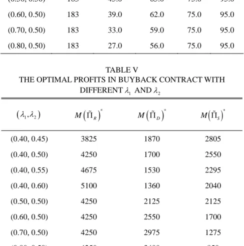
TABLE V

THE OPTIMAL PROFITS IN BUYBACK CONTRACT WITH DIFFERENTλ1 ANDλ2

(λ λ1, 2)

( )

*

R

M Π% M

( )

Π%D *

( )

*

S

M Π%

(0.40, 0.45) 3825 1870 2805

(0.40, 0.50) 4250 1700 2550

(0.40, 0.55) 4675 1530 2295

(0.40, 0.60) 5100 1360 2040

(0.50, 0.50) 4250 2125 2125

(0.60, 0.50) 4250 2550 1700

(0.70, 0.50) 4250 2975 1275

(0.80, 0.50) 4250 3400 850

From Tables IV and V, we can see that:

(6) The change of the values of parametersλ₁andλ₂will not impact on the optimal order quantity_q*

. (7) The wholesale prices *

1

w and * 2

w , and the return prices *

1

b and * 2

b will decrease with the increasing of the value of parameterλ₂, whenλ₁is fixed. With the increasing ofλ1, the wholesale price

* 1

w and the return price * 1

b will decrease, and the wholesale price *

2

w and the return price *

2

b will not vary, whenλ2is fixed.

(8) With the increasing ofλ₂, the optimal weighted possibilistic mean value of the fuzzy profit for the retailer will increase, and the optimal weighted possibilistic mean values of the fuzzy profits for the distributor and the supplier will decrease, whenλ1is fixed. Therefore, for the

retailer, he should seek as high value of parameterλ₂ as possible. Conversely, for the distributor or the supplier, he should seek as low value of parameterλ₂as possible. With the increasing ofλ1, the optimal weighted possibilistic mean

value of the fuzzy profit for the retailer will not vary, whenλ2is fixed. The optimal weighted possibilistic mean

value of the fuzzy profit for the distributor will increase as

1

λ increases. Therefore, for the distributor, he should seek as high value of parameterλ₁as possible. The optimal weighted possibilistic mean value of the fuzzy profit for the supplier will decrease as λ1increases. Therefore, for the supplier, he

IAENG International Journal of Applied Mathematics, 46:4, IJAM_46_4_16

[image:8.595.44.291.331.512.2]

(9)

should seek as low value of parameterλ1as possible.

V. 4BCONCLUSIONS

This article deals with the buyback contract with fuzzy demand in a three level supply chain, where the risk attitudes of the actors are considered. For examining the performance of supply chain members in the models, the weighted possibilistic mean value method is used to solve fuzzy models. We find that the change of the risk basic coefficient does not impact on the wholesale prices and return prices. The optimal weighted possibilistic mean value of the fuzzy profit for the supply chain actors vary with the changing of the risk basic coefficient and the values of contract parameters. One limitation of this article is that we only consider one supplier, one distributor and one retailer. Therefore, one possible extension work is to study the buyback contract with multiple competing retailers, distributors or suppliers in a fuzzy decision making environment. The other limitation is that the market demand of the supply chain models is considered as a trapezoidal fuzzy number. In fact, the membership function of the fuzzy number can be nonlinear, one can consider the case the demand is a fuzzy random variable.

REFERENCES

[1] T.M. Choi, D. Li and H. Yan, “Optimal returns policy for supply chain with e-marketplace”, International Journal of Production Economics, vol. 88, no.2, pp. 205–229, 2004.

[2] D. Ding and J. Chen, “Coordinating a three level supply chain with flexible return policies”, Omega,vol. 36, no.5, pp. 865–876, 2008. [3] J. Chen, “The impact of sharing customer returns information in a

supply chain with and without a buyback policy”, European Journal of Operational Research, vol. 213, no.3, pp. 478–488, 2011. [4] J. Chen and P.C. Bell, “Implementing market segmentation using

full-refund and no-refund customer returns policies in a dual-channel supply chain structure”, International Journal of Production Economics,vol. 136, no.1, pp. 56–66, 2012.

[5] Y. Zhao, T.M. Choi, T.C.E. Cheng, S.P. Sethi and S. Wang, “Buyback contracts with price-dependent demands: Effects of demand uncertainty”, European Journal of Operational Research, vol. 239, no.3, pp. 663–673, 2014.

[6] L. Xu, Y. Li, K. Govindan and X. Xu, “Consumer returns policies with endogenous deadline and supply chain coordination”, European Journal of Operational Research, vol. 242, no.1, pp. 88–99, 2015. [7] Z. Yao, S.C.H. Leung and K.K. Lai, “Analysis of the impact of

price-sensitivity factors on the returns policy in coordinating supply chain”, European Journal of Operational Research, vol. 187, no.1, pp. 275–282, 2008.

[8] H. Gurnani, A. Sharma and D. Grewal, “Optimal returns policy under demand uncertainty”, Journal of Retailing, vol. 86, no.2, pp. 137–147, 2010.

[9] J. Chen and P. C. Bell, “Coordinating a decentralized supply chain with customer returns and price-dependent stochastic demand using a buyback policy”, European Journal of Operational Research, vol. 212, no.2, pp. 296–300, 2011.

[10] F. J. Arcelus, S. Kumar and G. Srinivasan, “Channel coordination with manufacturer’s return policies within a newsvendor framework”,

4OR, vol. 9, no.3, pp. 279–297, 2011.

[11] X. Ai, J. Chen, H. Zhao and X. Tang, “Competition among supply chains: Implications of full returns policy”, International Journal of Production Economics, vol. 139, no.1, pp. 257–265, 2012.

[12] D. Wu, “Coordination of competing supply chains with news-vendor and buyback contract”, International Journal of Production Economics, vol. 144, no.1, pp. 1–13, 2013.

[13] X. Huang, J.W. Gu, W.K. Ching and T.K. Siu, “Impact of secondary market on consumer return policies and supply chain coordination”,

Omega, vol. 45, no.5, pp. 57–70, 2014.

[14] T.M. Choi, D. Li and H. Yan, “Mean–variance analysis of a single supplier and retailer supply chain under a returns policy”, European

Journal of Operational Research, vol. 184, no.1, pp. 356–376, 2008. [15] C.C. Hsieh and Y.T. Lu, “Manufacturer’s return policy in a two-stage

supply chain with two risk-averse retailers and random demand”,

European Journal of Operational Research, vol. 207, no.1, pp. 514–523, 2010.

[16] S.H. Yoo, “Product quality and return policy in a supply chain under risk aversion of a supplier”, International Journal of Production Economics, vol. 154, pp. 146–155, 2014.

[17] Y. Yu and T. Jin, “The return policy model with fuzzy demands and asymmetric information”, Applied Soft Computing, vol. 11, no.2, pp. 1669–1678, 2011.

[18] Y. Yu, J. Zhu and C. Wang, “A newsvendor model with fuzzy price-dependent demand”, Applied Mathematical Modelling, vol. 37, no.5, pp. 2644–2661, 2013.

[19] S.Y. Chang and T.Y. Yeh, “A two-echelon supply chain of a returnable product with fuzzy demand”, Applied Mathematical Modelling, vol. 37, no.6, pp. 4305–4315, 2013.

[20] S. Sang, “Supply chain contracts with multiple retailers in a fuzzy demand environment”, Mathematical Problems in Engineering, vol. 2013, pp. 1–12, 2013.

[21] B. Zhang, S. Lu, D. Zhang and K. Wen, “Supply chain coordination based on a buyback contract under fuzzy random variable demand”,

Fuzzy Sets and Systems, vol. 255, no.16, pp. 1-16, 2014.

[22] H. Yano, K. Matsui and M. Furuhashi, “Multi-objective fuzzy random linear programming problems based on coefficients of variation,” IAENG International Journal of Applied Mathematics, vol.44, no 3, pp. 137-143, 2014.

[23] S. Sang, “Coordinating a three stage supply chain with fuzzy demand” Engineering Letters, vol.22, no 3, pp. 109-117, 2014.

[24] M.F. Yang, M.C. Lo and W.H. Chen, “Optimal strategy for the three-echelon inventory system with defective product, rework and fuzzy demand under credit period” Engineering Letters, vol.23, no4, pp. 312–317, 2015.

[25] C. Carlsson and R. Fuller, On possibilistic mean value and variance of fuzzy numbers, Fuzzy Sets and Systems, vol. 122, no.2, pp. 315-326, 2001.

Shengju Sang is an associate professor at Department of Economics and Management, Heze University, Heze, China. He received his Ph.D. degree in 2011 at the School of Management and Economics, Beijing Institute of Technology, China. His research interest includes supply chain management, fuzzy decisions and its applications. He is an author of several publications in these fields such as Fuzzy Optimization and Decision Making, Journal of Intelligent & Fuzzy Systems, Springer Plus, Mathematical Problems in Engineering and other journals.