Abstract—Two fifth-order explicit hybrid methods are developed. Based on these methods, phase fitted and amplification fitted methods are constructed by vanishing both the phase-lag and the dissipation error. For the phase fitted and amplification fitted methods, computation of the output stage is dependent on the frequency of the problem being solved, thus the methods can only be applied when the frequency is known in advance. Numerical comparisons that have been carried out show the advantage of the new methods for solving several second-order ordinary differential equations with oscillating solutions.
Index Terms—hybrid methods, second-order ordinary differential equations, zero dissipation error, zero phase-lag
I. INTRODUCTION
N this paper, we are interested in the research on numerical methods for solving second order ordinary differential equations of the form
x f
x,y
x
,yx0 y0,y
x0 y0y
where the first derivative does not appear explicitly. These problems often arise in engineering and applied sciences such as celestial mechanics, quantum mechanics, elastodynamics, theoretical physics, chemistry and electronics and can be solved by using Runge Kutta Nystrom methods (see for example Senu [1]) and multistep methods. Several authors such as Fatunla, et. al. [2], Chawla [3], Tsitouras [4] and Simos [5] proposed hybrid methods which are obtained from the idea underlying both the Runge Kutta and linear multistep methods.
In the developments of hybrid methods, it is important to increase the order of the methods to achieve higher accuracy. In addition, if the second order ordinary differential equations have oscillating solutions, then it is also essential to consider the phase-lag and the dissipation error that result from comparing the numerical solution with
Manuscript received April 22, 2013; revised June 20, 2013. This work was supported by Ministry of Higher Education Malaysia under Research Acculturation and Collaboration Effort (RACE) grant scheme.
F. Samat is a lecturer at the Mathematics Department, Faculty of Science and Mathematics, Universiti Pendidikan Sultan Idris, 35900 Tanjong Malim, Perak, Malaysia (e-mail: faieza77@ yahoo.com or [email protected]).
F. Ismail is a lecturer at the Mathematics Department, Faculty of Science, Universiti Putra Malaysia, 43400 Serdang, Selangor, Malaysia (e-mail: [email protected]).
M. Suleiman is a fellow researcher at the Institute for Mathematical Research, Universiti Putra Malaysia, 43400 Serdang, Selangor, Malaysia (e-mail: [email protected]).
the analytical solution. These are actually two types of truncation errors. The first is the angle between the analytical solution and the numerical solution while the second is the distance from a standard cyclic solution. The study of phase-lag has been initiated by Brusa and Nigro [6]. The research of hybrid methods has been carried out by many authors paying attention to obtain methods with minimal phase-lag or with zero dissipation error (see [7] to [11]).
Consider the class of hybrid methods:
s j
j j n j n
n
n y y h b f x c h g
y
1 2 1
1 2 , (1)
with
s
j
j j n ij n
i n i
i c y cy h a f x c h g
g
1 2
1 ,
1
This class of methods has been discussed in many papers (for example see [4,12,13]). By assuming c1 = 1 and c2 = 0,
Tsitouras [4] derived an eight-order implicit hybrid method. Meanwhile, Franco [13] proposed a class of explicit hybrid methods by assuming c1 = 1 and c2 = 0. In [14], Fang et. al.
derived one- frequency and two-frequency explicit hybrid methods based on the fifth-order hybrid method in [13]. The coefficients of the new methods in [14] are obtained by vanishing both the phase-lag and the dissipation error.
Here, inspired by Runge Kutta methods, we choose c1 =
0 and c2 = 1. The class of explicit hybrid methods with c1 =
0 and c2 = 1 can be represented by the Butcher tableau:
s
c c
3
1 0
0 0 0
0 0
0
0 0
0 0
1 , 2
1 32 31 21
s s s
s a a
a a a a
= c A
b1 b2 bs1 bs
The leading term associated with the local truncation error of a p-th order hybrid method is given as
1
1
, , !2 2
2
1 t t T
p t t
e i i
T p i
i
p
b
ti p2 where T2, (ti) and
ti are as defined in[12]. The quantity
2
1 2
1
p n
i
i p t e E
where np+2 is the number of trees of order p + 2, is called the
error constant for the p-th order method. Based on this class of methods, we derive fifth order explicit hybrid methods
Phase fitted and Amplification fitted Hybrid
Methods for Solving Second-order Ordinary
Differential Equations
F. Samat, F. Ismail and M. Suleiman
I
bT
IAENG International Journal of Applied Mathematics, 43:3, IJAM_43_3_02
with four stages (s = 4). Then, based on these methods, we derive phase fitted and amplification fitted explicit hybrid methods. The phase fitted and amplification fitted methods are obtained by vanishing the phase-lag and the dissipation error. The implementation of the methods is investigated by comparing the accuracy of the methods with that of the base and other existing methods.
II. PHASE-LAG ANALYSIS
Let Hh and e
1 1 1
T. Applying the hybrid methods defined in (1) to equationy2y, 0 yields the recursion
2
2 1 01
n n
n S H y PH y
y (2) where
H2 2H2b
IH2A
1
ec
S T
andP
H2 1H2bT
IH2A
1c.The characteristic equation associated with (2) is
2
2 02
H P H
S
(3) According to Houwen and Sommeijer [15], phase-lag is
defined as the difference
H Ht
where H is the phase (or argument) of the exact solution of y
y2
and
H is the phase of the principal root of (3). In case for explicit methods, the matrix A is nilpotent of degree s (that is As = O). Therefore,
2
1 2 4 2 6 3 2s2 s1A H A H A H A H I A H
I .
For the hybrid methods corresponding to the characteristic equation (3), the quantity
2 2 2 arccos H P H S H H is called phase-lag (or dispersion error) while the quantity
21 PH H
d
is called dissipation (or amplification) error. A hybrid method corresponding to (3) is said to have the phase-lag of order n if
n1
H O H
. If
H 0 then the method is said to be phase fitted or zerodispersive. If P
H2 1 then
H 0d and the method having this property is said to be
amplification fitted or zero dissipative. If P
H2 1 then
H O
Hm1
d and the method with this property is said to be dissipative of order m.
The interval
0,Hp
is called the interval of periodicity of the method if
H2 1P and S
H2 2 for all H
0,Hp
whereas the method is called P-stable if
H2 1P and S
H2 2 for all H
0, . The interval
0,Ha
is called the interval of absolutestability if
H2 1P and
2
21 PH H
S for all H
0,Ha
.III. CONSTRUCTION OF HYBRID METHODS
A. Construction of Fifth-order Methods
In this section, fifth-order explicit hybrid methods are constructed. The following are order conditions that have to be satisfied (see [12]).
1 1
s i i b 0 1
s i i ic b 6 1 1 2
s i i ic b
s i s j ij ia b1 1 12
1
s i i ic b 1 3 0
s i s j ij i icab
1 1 12
1
s i s j j ij ia cb 1 1 0 15 1 1 4
s i i ic b 30 1 1 1 2
s i s j ij i ic ab
s i s j j ij i ica cb
1 1 60
1
120 7
1 1 1
s i s j s k ik ij ia ab 180 1 1 1 2
s i s j j ij ia cb
s i s j s k jk ij ia ab
1 1 1 360
1
Substituting s4,c10,c2 1,aij 0
ji
into theabove order conditions and solving the resulting equations using Maple software, we obtain
, 2 5 6 3 7 25 3 3 3 2 3 1 c c c c b
, 1 5 2 5 3 3 4 c cc
,1 10 7 6 2 5 3 3 2 3 2 c c c b
1
10 2 5
, 2 1 2 3 3 3 3 3 c c c c b
, 5 2 10 2 5 10 7 6 1 125 2 3 3 3 3 4 3 4 c c c c c b a21 1,
, 2 1 6 1 3 2 2 3 3 3 3
31 c c c
a
1
1
, 61
3 3 3
32 c c c a
1
,3750 14 240 570 325 2 5 4 3 3 3 2 3 3 3 3 41 c c c c c c a
1
1
,3750 10 10 17 10 7 2 5 3 4 3 3 2 3 3 3 42 c c c c c c a
IAENG International Journal of Applied Mathematics, 43:3, IJAM_43_3_02
1
1
.3750
5 2 10 2 5 10 7
3 4 3 3
2 3 3
3 3 43
c c
c
c c
c c a
For the first method, the free parameter c3 is chosen so that
the error constant E, is as small as possible giving us
2 3 , 1.85 10
100
69
E
c
The new method will be denoted by EHM5I. Coefficients of EHM5I method are displayed in Table I.
The phase-lag order and the dissipation order for this method are six and five respectively with the following quantities
,1512000
71 7 9
H O H
H
.216000
31 6 12
H O H H
d
The interval of absolute stability is (0, 3.36).
For the second method, the free parameter c3 is chosen so
that the phase-lag order is eight. This gives us the values
2 3 , 7.09 10
28
25
E
c
The new method is denoted by EHM5II. Coefficients of EHM5II method are shown in Table II.
This method has phase-lag of order eight and is dissipative of order five with the following quantities
9
117257600 17
H O H
H
6
1220160 1
H O H H
d
The interval of absolute stability is (0, 3.94).
B. Construction of Phase Fitted and Amplification Fitted Methods
Here, phase fitted and amplification fitted hybrid methods denoted by EHM5IPA and EHM5IIPA will be derived. The derivations of EHM5IPA and EHM5IIPA are being based on EHM5I and EHM5II methods respectively. Table III shows coefficients of EHM5IPA method.
It is noted that some of the values are taken from Table I. The coefficients b1 and b2 are obtained by vanishing the
phase-lag and the dissipation error. The quantity S
H2 has to be equal to 2cos
H P
H2 in order to vanish the phase-lag. Solving the resulting equation, we get
157170 205470000
. 547560000
547560000 cos
1040520 0
2434816800
0 2434816800 37311313
3494413 0
1217408400
5582790000 0
1305162000 0
1217408400 1
2 1 2 6
2 2
2 2 6
8 2
4
4 2
2 1
H H
H b H
H H
b H H
H H
b H
H H
H b
For the dissipation error to vanish, we set
2 1H
P and
then solve the resulting equation giving
2028 761 108000
31 4
2 H
b .
For small H, the coefficient b1 is subject to heavy cancellations. Therefore, it is convenient to use the Taylor series expansion:
. 0
4358914560 1 239500800
1
1814400 1 20160
1 108000
31 1334
905
12 10
8 6
4 1
H H
H H
H b
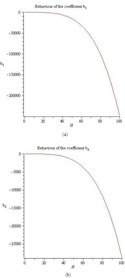
Behaviour of the coefficients is given in Fig. 1. TABLEI
COEFFICIENTS OF EHM5I
31 29 100
69 1 0
0 3 3230753514
292262000 468225147
6193240 191168847
173865730
0 0
2000000 120497 2000000
3343971 0 0 0
0 0
0 0
1753572 923521 58759779
10000000 2028
761 1334
905
TABLEII COEFFICIENTS OF EHM5II
5 2328
25 1 0
0 828125 13866608 33125
16744 15625
454986
0 0
43904 1325 43904
34251 0 0 0
0 0
0 0
636732 125 3056775
307328 1908
173 3450
2791
TABLEIII COEFFICIENTS OF EHM5IPA
31 29100
69 1 0
0 3 3230753514
292262000 468225147
6193240 191168847
173865730
0 0
2000000 120497 2000000
3343971 0 0 0
0 0
0 0
1753572 923521 58759779
10000000
2 1 b b
IAENG International Journal of Applied Mathematics, 43:3, IJAM_43_3_02
Fig. 1. Behaviour of the coefficients b1 and b2 of the new proposed method;
EHM5IPA for several values of H = h.
Let us consider coefficients of EHM5IIPA given by Table IV.
Some of the values in Table IV are taken from Table II. Using the similar procedure, by vanishing the phase-lag, we obtain
12
2 62 2
2 2
6 8
2 4
4 2
2 1
179712400 196630
1982030400
1982030400 cos
2760 122875200
122875200 176755
6095 61437600
450800 594272
61437600 1
H H
b H
H b
H
H H
b H
H H
H b
whereas by vanishing the dissipation error,
whereas by vanishing the dissipation error, . 1908
173 10080
1 4
2 H b
The Taylor series expansion for b1 is given by
12 10
8 6
4 1
0 4358914560
1 239500800
1
1814400 1 20160
1 10080
1 3450 2791
H H
H H
H b
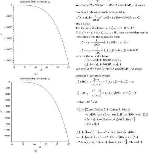
The behaviour of the coefficients is given in Fig. 2.
IV. NUMERICAL RESULTS
All new codes have been applied to some second-order problems to provide numerical comparisons with other competitive codes in the scientific literature. Codes that have been used for numerical comparisons are denoted by: EHM5I : The first fifth-order explicit hybrid method with four stages derived in this paper. This method has phase-lag of order six and is dissipative of order five. The interval of absolute stability is (0, 3.36).
EHM5II : The second fifth-order explicit hybrid method with four stages derived in this paper. This method has phase-lag of order eight and is dissipative of order five. The interval of absolute stability is (0, 3.94)
EHM5IPA : The phase fitted and amplification fitted explicit hybrid method which is derived based on EHM5I in this paper.
EHM5IIPA : The phase fitted and amplification fitted explicit hybrid method which is derived based on EHM5II in this paper.
FETSH : The fifth-order explicit hybrid method with three stages derived by Franco [13]. This method has phase-lag of order eight and is dissipative of order five. The interval of absolute stability is (0, 2.84) whereas the formula for this method is given by
3 3
4
4 4
3
2 1 1 2 1 1
3 3 43
42 1 41 2 1 4 4 4
32 1 31 2 1 3 3 3
2 1 1
, ,
2
,
1 1
,
Y h c x f b Y h c x f b
f b f b h y y y
Y h c x f a
f a f a h y c y c Y
f a f a h y c y c Y
y Y y Y
n n
n n
n n n
n
n n
n n
n n
n n
n n
The coefficients of the method can be found in [13].
TSI7: The seventh-order explicit hybrid method with four stages derived in [16]. This method has the form
n n
n f x y f , , TABLEIV
COEFFICIENTS OF EHM5IIPA
5 23
28 25 1 0
0 828125 13866608 33125
16744 15625
454986
0 0
43904 1325 43904
3425
0 0
0 1
0 0
0 0
636732 125 3056775
307328
2
1 b
b
IAENG International Journal of Applied Mathematics, 43:3, IJAM_43_3_02
n
n n
n
a c y c y h d f d f
y 2 11 1 12
1 1
1 1
,
fa f
xn c1h,ya
,
, 1 21 22 1 21 2 2 1 2 a n n n n b f g f d f d h y c y c y
n 2 , b
, b f x c h yf
, 1 32 31 32 1 31 2 3 1 3 b a n n n n c f g f g f d f d h y c y c y
n 3 , c
, c f x c h yf
. 2 3 2 1 2 1 1 2 1 1 c b a n n n n n f b f b f b f w f w h y y y [image:5.595.51.571.266.786.2]The coefficients can be found in [16]. According to Tsitouras [16], the coefficients of this method have been selected so that the local truncation error is minimized.
Fig. 2. Behaviour of the coefficients b1 and b2 of the new proposed method;
EHM5IIPA for several values of H = h.
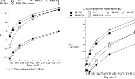
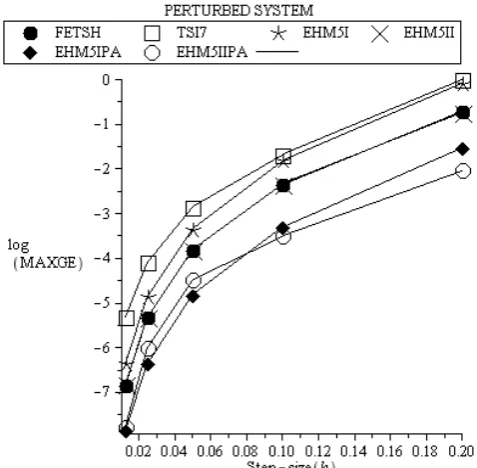
Criterion used as a measure for accuracy is the maximum global error given by the formula
MAXGE = max y
xn ynwhere y(xn) is the exact solution and yn is the computed solution. The numerical results are given in Fig. 3 to 6. Test problems that have been used are as follows.
Problem 1 (non-homogeneous problem)
, 0 1,
0 11, 0 100sin 99
100
y x y y x
y
Solution: y
x cos
10x sin
10x sin
x .We choose H = 10h for EHM5IPA and EHM5IIPA codes. Problem 2 (homogeneous problem)
0 0,
0 1, 0 100 ,2500
y y y x
y
Solution: y
x sin
50x 501
.
We choose H = 50h for EHM5IPA and EHM5IIPA codes. Problem 3 (almost periodic orbit problem)
. 100 0 , , 9995 . 0 0 , 1 0 , 1000 1 x z i z z e x z xz ix C
The theoretical solution is z
x 10.0005ix
eix.If z
x y1
x iy2
x,y1,y2R, then the problem can be transformed into the equivalent form
, 0 0,
0 0.9995 sin 1000 1 0 0 , 1 0 , cos 1000 1 2 2 2 2 1 1 1 1 y y x y y y y x y ywith the theoretical solution:
. cos 0005 . 0 sin , sin 0005 . 0 cos 2 1 x x x x y x x x x y We choose H = h for EHM5IPA and EHM5IIPA codes. Problem 4 (perturbed system)
100 2 2 1 , 1 0 1, 10
2 2 1 2 1 1
1 f x y y
y y y y y y
, 0 ,
0 525 2 2 2
2 2 2 1 2 2 2 1 2
2
f x y y
y y y y y y
with103and
, sin 99 5 sin cos 10 cos sin 2 5 sin 10 cos / 2 sin cos 10 cos sin 5 sin 2 5 sin 10 cos 2 2 2 2 2 1 x x x x x x x x x x x x x x x f
sin cos10 cos sin5
24 cos
. 2 5 sin 10 cos / 2 cos 5 sin cos 10 cos sin 2 5 sin 10 cos 2 2 2 2 2 2 2 x x x x x x x x x x x x x x x f IAENG International Journal of Applied Mathematics, 43:3, IJAM_43_3_02
Solution:
. 10 0
, cos 5
sin ,
sin 10
cos 2
1
x
x x
x y x x
x
y
For EHM5IPA and EHM5IIPA codes, we choose H = 10h
for the first component and H = 5h for the second component.
[image:6.595.308.545.54.289.2]From the numerical results, it is observed that EHM5I is almost as accurate as FETSH method. In addition, the maximum global error for EHM5II is of the same order as that for FETSH method with advantage for EHM5II as EHM5II is more stable for solving Problem 2. For Problem 3, EHM5IPA is the most accurate followed by TSI7. TSI7 is unstable when it was used to solve Problem 2 and Problem 4 for big step-size. Of all methods, EHM5IPA and EHM5IIPA are the most accurate for solving most problems considered. This is because EHM5IPA and EHM5IIPA are being phase fitted and amplification fitted compared to other methods.
[image:6.595.51.306.294.527.2]Fig. 3. Numerical results for Problem 1
Fig. 4. Numerical results for Problem 2
Fig. 5. Numerical results for Problem 3
IAENG International Journal of Applied Mathematics, 43:3, IJAM_43_3_02
[image:6.595.83.537.305.571.2]Fig. 6. Numerical results for Problem 4
V. CONCLUSION
In this paper, we investigate the implementation of phase fitted and amplification fitted explicit hybrid methods for solving second order ordinary differential equations. From numerical observations, we conclude that the phase fitted and amplification fitted explicit hybrid methods are very accurate for solving second-order ordinary differential equations having oscillating solutions. The results also indicate that phase fitting and amplification fitting gives us methods with better accuracy compared to the base methods. Moreover, all of the new methods are capable to solve any physical problems whose solutions are in the oscillatory form. All codes are designed using Microsoft Visual C++ version 6.0 software in HP computer with
specification Intel(R)Core(TM)2DuoCPU [email protected].
REFERENCES
[1] N. Senu, M. Suleiman, F. Ismail and M. Othman, “A singly diagonally implicit Runge Kutta Nystrom method for solving oscillatory problems,” IAENG International Journal of Applied Mathematics, vol. 41, no. 2, pp. 155-161, May 2011. Available: http://www.iaeng.org/IJAM/issues_v41/issue_2/IJAM_41_2_11.pdf [2] S. O. Fatunla, M. N. O. Ikhile and F. O. Otunta, “A class of P-stable
linear multistep numerical methods,” International Journal of Computer Mathematics, vol. 72, pp. 1-13, 1999.
[3] M. M. Chawla, “Numerov made explicit has better stability,” BIT24, pp. 117-118, 1984.
[4] Ch. Tsitouras, “Stage reduction on P-stable Numerov type methods of eighth order,” Journal of Computational Applied Mathematics, vol. 191, pp. 297-305, 2006.
[5] T. E. Simos, “Optimizing a hybrid two-step method for the numerical solution of the Schrodinger equation and related problems with respect to phase-lag,” Journal of Applied Mathematics, Article ID 420387. 17 pages, 2012. Available:
http://www.hindawi.com/journals/jam/2012/420387/ref/
[6] L. Brusa, and L. Nigro, “A one-step method for direct integration of structural dynamic equations,” International Journal for Numerical Methods in Engineering, vol. 15, pp. 685-699, 1980.
[7] J. M. Franco, “An explicit hybrid method of Numerov type for second order periodic initial-value problems,” Journal of Computational and Applied Mathematics, vol. 59, pp. 79-90, 1995.
[8] T. E. Simos, “Explicit two-step methods with minimal phase-lag for the numerical integration of special second-order initial-value problems and their application to the one-dimensional Schrödinger equation,” Journal of Computational and Applied Mathematics, vol. 39, pp. 89-94, 1992.
[9] T. E. Simos, I. T. Famelis and Ch. Tsitouras, “Zero dissipative, explicit Numerov-type methods for second order IVPs with oscillating solutions,” Numerical Algorithms, vol. 34, pp. 27-40, 2003.
[10] M. M. Chawla and P. S. Rao, “An explicit sixth-order method with phase-lag of order eight for y”=f(x,y),” Journal of Computational and Applied Mathematics, vol. 17, pp. 365-368, 1987.
[11] T. E. Simos and A. D. Raptis, “Numerov-type methods with minimal phase-lag for the numerical integration of the one-dimensional Schrödinger equation,” Computing, vol. 45, pp. 175-181, 1990. [12] J. P. Coleman, “Order conditions for a class of two-step methods for
y”=f(x,y),” IMAJournal of Numerical Analysis, vol. 23, pp. 197-220, 2003.
[13] J. M. Franco, “A class of explicit two-step hybrid methods for second-order IVPs,” Journal of Computational and Applied Mathematics, vol. 187, pp. 41-57, 2006.
[14] Y. Fang, X. You, Z. Chen, “New phase fitted and amplification fitted Numerov-type methods for periodic IVPs with two frequencies,”
Abstract and Applied Analysis, Article ID 742585. 15 pages, 2012. Available: http://www.hindawi.com/journals/aaa/2012/742585/ref/ [15] P. J. van der Houwen and B. P. Sommeijer, “Explicit Runge-Kutta
(-Nystrom) methods with reduced phase errors for computing oscillating solutions,” SIAM Journal of Numerical Analysis, vol. 24, pp. 595-617, 1987.
[16] Ch. Tsitouras, “Explicit two-step methods for second-order linear IVPs,” Computers and Mathematics with Applications, vol. 43, pp. 943-949, 2002.