First Order Fuzzy Transform for Images Compression

(1)

http://www.scirp.org/journal/jsip ISSN Online: 2159-4481

ISSN Print: 2159-4465

First Order Fuzzy Transform for

Images Compression

Ferdinando Di Martino

1

, Salvatore Sessa

2

, Irina Perfilieva

3

1_{Università degli Studi di Napoli Federico II, Dipartimento di Architettura, Napoli, Italy}

2_{Università degli Studi di Napoli Federico II, Centro Interdipartimentale di Ricerca Calza Bini, Napoli, Italy} 3_{University of Ostrava, Institute for Research and Applications of Fuzzy Modeling, Ostrava, Czech Republic}

Abstract

In this paper, we present a new image compression method based on the di-rect and inverse F1_{-transform, a generalization of the concept of fuzzy}

trans-form. Under weak compression rates, this method improves the quality of the images with respect to the classical method based on the fuzzy transform.

Keywords

Fuzzy Transform, Generalized Fuzzy Partition, Basic Function, Hilbert Space, Image Compression, PSNR

1. Introduction

We present a new image compression method based on the discrete direct and inverse F1_{-transform which is a generalization of the classical fuzzy transform}_[1]

[2] identified as F0_{-transform (for brevity, F-transform).}

The F-transform compression technique [3] is a lossy compression method used in image and video analysis [4]-[18] and in data analysis [19]-[25] as well. In [26], the concept of the F-transform was extended to the cases with various types of fuzzy partitions. In [1] [27], the Fs_{-transform (}_s_{≥ 1), a generalization of}

the F-transform, was presented: in other terms, the constant components of the F-transform were replaced by polynomials in order to capture more information of the original function. In particular, the F1_{-transform was used for the edge}

detection problem [1] [2]. The aim of this paper is to improve the quality of the decoded images after their compression via the F1_{-transform-based method.}

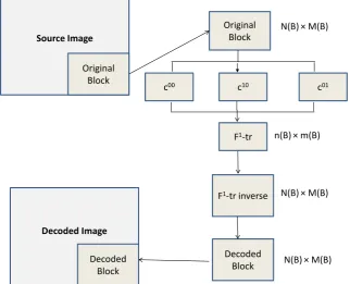
Strictly speaking, we divide images of sizes N × M into smaller images (called blocks) of sizes N(B) × M(B) and then we code each block into another one of sizes n(B) × m(B), where n(B) < N(B) and m(B) < M(B). The compression is How to cite this paper: Di Martino, F.,

Sessa, S. and Perfilieva, I. (2017) First Order Fuzzy Transform for Images Compression. Journal of Signal and Information Processing, 8, 178-194.

https://doi.org/10.4236/jsip.2017.83012

Received: May 16, 2017 Accepted: August 22, 2017 Published: August 25, 2017

(2)

performed by calculating the direct F1_{-transform components with first degree}

polynomials. Afterwards, we calculate the inverse F1_{-transform and obtain the}

corresponding decoded blocks, recomposed to obtain the final reconstructed image. In Figure 1, we describe this process in detail.

The compression rate is given by ρ=

(

n B

( )

×m B

( )

)

(

N B

( )

×M B

( )

)

. The

quality of a decoded image is measured by the Peak Signal to Noise Ratio (PSNR) index.

In Section 2, we recall the definition of h-uniform generalized fuzzy partition and the concept of F1_{-transform. In Section 3, a F}1_{-transform-based compression}

method is presented and it is applied to images considered as fuzzy relations: there every image is partitioned into smaller blocks and the direct and inverse F1_{-transforms are calculated for each block. Then the decoded blocks are}

re-composed and the PSNR index is calculated. In Section 4, tests are applied to grey image datasets and the results are compared with similar results obtained by using the classical F-transform compression method. Section 5 contains the conclusions.

2. Generalized Fuzzy Partition and F

1

_-Transform

We recall the main concepts [2] that will be used in the sequel. We consider a set of points (called nodes) x x x0, 1, 2,,x xn, n+1,n≥2 of

[ ]

a b, such that

0 1 2 n n1

a=x ≤x <x <<x ≤x+ =b. We say that the fuzzy sets

[ ] [ ]

1, , n: , 0,1

A  A a b → form a generalized fuzzy partition of

[ ]

a b, , if for each

1, 2, ,

k=  n, there exist h hk′ ′′ ≥, k 0 such that hk′+hk′′>0,

[image:2.595.213.536.451.712.2]

[

xk−h xk′, k+hk′′

] [ ]

⊆ a b, and the following constraints hold:

Figure 1. The F1_{-transform image compression method.} Original

Block

c00 _c10 _c01

Source Image

Original Block

Decoded Image

F1_{-tr inverse}

Decoded Block

F1_-tr

Decoded Block

N(B) × M(B)

n(B) × m(B)

N(B) × M(B)

(3)

1) (locality) A xk

( )

>0 if x∈

[

xk−h xk′, k+hk′′

]

and A xk

( )

=0 if

[

k k, k k

]

x∉ x −h x′ +h′′ ,

2) (continuity) Ak is continuous in

[

xk −h xk′, k+hk′′

]

,

3) (covering) for each x∈

[ ]

a b, ,

( )

1

0

n

k k

A x

=

>

∑

.

The fuzzy sets

{

A1,,An

}

are called basic functions. If the nodes 0, 1, , n, n1

x x  x x+ are equidistant, i.e. xk+1−xk =h for k=0,1, 2,,n, where

(

) (

1

)

h= b a− n+ , if h′ >h 2 and the following additional properties hold:

4) h1′=hn′′=0, h1′′=h2′==hn′′−1=hn′=h′and A xk

(

k−x

)

= A xk

(

k+x

)

for

each x∈

[ ]

0,h′ and k=2,,n,

5) A xk

( )

=Ak−1

(

x h−

)

and Ak+1

( )

x =A x hk

(

−

)

for every x∈

[

x xk, k+1

]

and k=2,,n, then

{

A1,,An

}

is called an

(

h h, ′

)

-uniform generalized

fuzzy partition. In this case we can find a function A0:

[ ] [ ]

−1,1 → 0,1, called

ge-nerating function, which is assumed to be even, continuous and positive every-where except on the boundaries, every-where it vanishes, in such a way we have that for k=1, 2,,n:

( )

0

[

,

]

0 otherwise.

k

k k

k

x x

A x x h x h

A x h

  −  _∈ ₋ ₊

  

=   

 

(1)

If h=h′, then the

(

h h, ′

)

-uniform generalized fuzzy partition is said

h-uniform generalized fuzzy partition. We can extend the notion of h-uniform generalized fuzzy partition from an interval to the rectangle

[ ] [ ]

a b, × c d, , so

that we have the family of basic functions

{

Ak×B kl, =1,, ,n l=1,, ; ,m n m≥2

}

,

where Ak×Bl is the product of the corresponding functions from the h1-uniform

generalized fuzzy partition

{

A1,,An

}

of

[ ]

a b, and from the h2-uniform

ge-neralized fuzzy partition

{

B1,,Bm

}

of

[ ]

c d, . Then we can say that

{

Ak×B kl, =1,, ,n l=1,, ; ,m n m≥2

}

is an h-uniform generalized fuzzy

parti-tion of

[ ] [ ]

a b, × c d, , where h= ⋅h h₁ ₂. In the sequel we consider only such

h-uniform generalized fuzzy partitions.

Let A xk

( )

be a basic function of

[ ]

a b, and L2

( )

Ak be the Hilbert space

of square integrable functions f :

[

xk−1,xk+1

]

→R (reals) with weighted inner

product:

( ) ( ) ( )

1

, d

k

x

k k

x

f g f x g x A x x

+

−

=

_∫

Likewise, we define the Hilbert space L2

(

Ak×Bl

)

of square integrable in two

variables functions f :

[

xk−1,xk+1

] [

× yl−1,yl+1

]

→R with weighted inner

prod-uct:

( ) ( ) ( ) ( )

1 1

, d d

k l

x y

k l

kl x y

f g f x g x A x B y x y

+ +

− −

=

_{∫ ∫}

₍₂₎

Two function f g, ∈L2

(

Ak×Bl

)

are orthogonal if f g, kl =0. Let 2

( )

p

k L A

and 2

( )

r

l

L B , p r, ≥0 be two linear subspaces of L2

( )

Ak and L2

( )

Bl with

orthogonal basis given by polynomials

{

i

( )

}

_0, _,

k _i _p

P x

=  and

{

( )

}

0, , j

k _j _r

Q y

(4)

re-spectively.

We consider an integer s≥0 and all pairs of integers (i, j) such that

0≤ + ≤i j s. We introduce a linear subspace 2

(

)

s

k l

L A ×B of L₂

(

A_k×B_l

)

having as orthogonal basis the following:

( )

( ) ( )

{

,

}

0, , ; 0, , :

ij i j

kl k l _i _{p j} _{r i j s} S x y P x Q y

= = + ≤

=

  (3)

where s is the maximum degree of polynomials

( ) ( )

l

i j

k

P x Q y . For s = 1, the

or-thogonal basis of the linear space 1

(

)

2 k l

L A ×B is the following:

( )

( ) ( )

( )

( ) ( )

( )

( ) ( )

{

00 0 0 10 1 0 01 0 1

}

l l l

, , , , ,

kl k kl k kl k

S x y =P x Q y S x y =P x Q y S x y =P x Q y (4)

Let L2

(

[ ] [ ]

a b, × c d,

)

be a set of functions f :

[ ] [ ]

a b, × c d, →R such that

for k=1,,n, l=1,,m, f |

[

xk−1,xk+1

] [

× yk−1,yk+1

]

∈L2

( )

Ak ×L B2

( )

l ,

where the function f |

[

xk−1,xk+1

] [

× yk−1,yk+1

]

is the restriction of f on

[

xk−1,xk+1

] [

× yk−1,yk+1

]

. Then the following theorem holds:

Theorem 1. ([2], lemma 5). Let f ∈L2

(

[ ] [ ]

a b, × c d,

)

. Then the orthogonal

projection of f on 2

(

)

s

k l

L A ×B , s≥0, is the polynomial of degree s given by

( )

0

, ,

s ij ij

kl kl kl

i j s

F x y c S x y

≤ + ≤

=

∑

(5)

for every

( )

x y, ∈

[ ] [ ]

a b, × c d, , where the coefficients ij kl

c are given by

( ) ( ) ( ) ( )

( )

(

)

( ) ( )

1 1 1 1 1 1 1 1 2

, , d d

, d d

l k l k l k l k y x ij

kl k l

y x ij

kl y x ij

kl k l

y x

f x y S x y A x B y x y

c

S x y A x B y x y

+ + − − + + − − =

∫ ∫

(6)

Following [2], let

{

Ak×B kl, =1,, ,n l=1,, , ,m n m≥2

}

be an h-uniform

generalized fuzzy partition of

[ ] [ ]

a b, × c d, and f∈L₂

(

A_k×B_l

)

. For s = 1, the

orthogonal basis of the linear subspace 1

(

)

2 k l

L A ×B is given by the

polyno-mials:

( )

( ) ( )

( )

( ) ( )

( )

( ) ( )

00 0 0

10 1 0

01 0 1

, 1

,

kl k l

kl k l k

kl k l l

S x y P x Q y

S x y P x Q y x x

S x y P x Q y y y

= =

= = −

(7)

Let 1 kl

F be the orthogonal projection of f |

[

xk−1,xk+1

] [

× yk−1,yk+1

]

on

(

)

1

2 k l

L A ×B given point wise as

( )

(

)

(

)

1 00 10 01

0 1

, ij ij ,

kl kl kl kl kl k kl l

i j

F x y c S x y c c x x c y y

≤ + ≤

=

∑

= + − + − (8)

for every

( )

x y, ∈

[ ] [ ]

a b, × c d, , where the three coefficients c_kl00,c_kl10,c_kl01 are

de-fined by Theorem 1:

( ) ( ) ( )

( )

1 1 1 1 1 1 1 1 00

, d d

d d l k l k k l k l y x k l y x

kl x y

k l

x y

f x y A x B y x y

c

A x x B y y

(5)

( )(

) ( ) ( )

( )(

)

( )

1 1 1 1 1 1 1 1 10 2

, d d

d d l k l k k l k l y x

k k l y x

kl x y

k k l

x y

f x y x x A x B y x y

c

A x x x x B y y

+ + − − + + − − − = −

∫ ∫

∫

(10)

( )(

) ( ) ( )

( )

( )(

)

1 1 1 1 1 1 1 1 01 2

, d d

d d l k l k k l k l y x

l k l y x

kl x y

k l l

x y

f x y y y A x B y x y

c

A x x B y y y y

+ + − − + + − − − = −

∫ ∫

∫

(11)

Then the matrix 1

[ ]

(

1 1

)

11, ,

nm f = F Fnm

F  , defined from (8), is called

F1_{-transform of the function}

(

)

2 k l

f ∈L A ×B with respect to the h-uniform

generalized fuzzy partition

{

Ak×B kl, =1,, ,n l=1,, ; ,m n m≥2

}

. We define

the inverse F1_{-transform of the function}

(

)

2 k l

f ∈L A ×B to be a function

[ ] [ ]

1

ˆ _: _, _,

nm

f a b × c d →R as

(

)

(

) ( ) ( )

( ) ( )

1

1 1 1

1 1

,

ˆ _,

n m

nm k l

k l

nm n m

k l

F x y A x B y

f x y

A x B y

= =

=

∑∑

(12)

For sake of completeness, we point out the utility of the concept of inverse F1_{-transform which stands in the approximation of the function}

(

)

2 k l

f∈L A ×B under certain suitable assumptions. For example, we have the

following result:

Theorem 2. ([2], theorem 14). Let

( ) ( )

(

)

{

Ak x B y, l ,k=1,, ,n l=1,, , ,m n m≥2

}

be an h-uniform generalized

fuzzy partition of

[ ] [ ]

a b, × c d, and _ˆ1 nm

f be the inverse F1-transform of f

with respect to this fuzzy partition. Moreover let f be four times continuously

differentiable on

[ ] [ ]

a b, × c d, and A_k (resp., B_l) be four times continuously

differentiable on

[ ]

a b, (resp.,

[ ]

c d, ). Then the following holds for every

( )

x y, ∈

[ ] [ ]

a b, × c d, :

(

_,

)

_ˆ1

(

_,

)

( )

2 nm

f x y −f x y =O h (13)

In other words, the Equality (13) says that we can approximate a function in two variables, four times continuously differentiable on

[ ] [ ]

a b, × c d, , with the

inverse F1_{-transform (12) unless to O (h}2_).

3. F

1

_{-Transform Image Compression Method}

We are interested to the case discrete, i.e. we consider functions in two variables which assume a finite number of values in

[ ]

0,1 like finite fuzzy relations.

In-deed, let R be a grey image of sizes N×M ,

( ) {

} {

}

[ ]

: , 1, , 1, , 0,1

R i j ∈  N ×  M → , R i j

( )

, =Rij being the normalized

value of the pixel P i j

( )

, , that is R i j

( )

, =P i j

( )

, Nlev if Nlev is the length of

the grey scale. Let

{

A1,,An

}

and

{

B1,,Bm

}

be two h-uniform generalized

(6)

b=N, xk =k k, =1, 2,, ,n nN, c=1, d =M, yl =l l, =1, 2,, ,m mM.

Slightly modifying (8), then we can define the (discrete) F1_-transform

1 1

nm kl _{n m}

R R

×

 

=   of R the matrix whose entries are defined as

1 00 10 01

kl kl kl kl

R =c +c ⋅ − +i k c j l− (14)

where 00 kl c , c10kl,

01 kl

c are given as (by rewriting the Equations (9), (10), (11) in

the following form, slightly modified):

( ) ( )

1 1 00 1 1 M N

ij k l j i

kl M N

k l j i

R A i B j c

A i B j

= =

=

∑∑

(15)

( ) ( )

( )(

)

( )

1 1 10 2 1 1 M N

ij k l

j i

kl N M

k l

i j

R i k A i B j c

A i i k B j

= = = = − = −

∑∑

∑

(16)

( ) ( )

( )

( )(

)

1 1 01 2 1 1 M N

ij k l

j i

kl N N

k l

i j

R j l A i B j c

A i B j j l

= = = = − = −

∑∑

∑

(17)

The Formula (14) is considered as a compressed image of the original image R.

1 nm

R can be decoded by using the following inverse (discrete) F1-transform

1 1

NM ij _{N M}

R R

×

 

=   defined for every

( ) {

i j, 1,∈ ,N

} {

× 1,,M

}

as

( ) ( )

1

1 1 1

1 1

n m

kl k l k l

ij n m

k l

R A i B j

R

A i B j

= =

=

∑∑

(18)

We divide the image R of sizes N×M in sub-matrices RB of sizes N B

( )

×M B

( )

,

called blocks ([26] [28]), each compressed to a block 1B _{( ) ( )} kl _{n B} _{m B}

R

×

 

  of sizes

( ) ( )

n B ×m B

(

3≤n B

( )

<N B

( )

, 3≤m B

( )

<M B

( )

)

, k=1,,n B

( )

,

( )

1, ,

l=  m B , via the discrete F1-transform, as Formula (14), of components

1B kl

R given by

1B 00B 10B 01B

kl kl kl kl

R =c +c i k− +c j l− (19)

We rewrite (15), (16), (17) as

( ) ( )

( ) ( ) 1 1 00 1 1 M B N B

B ij k l j i

B

kl M B N B

k l j i

R A i B j c

A i B j

= =

=

∑ ∑

(20)

( ) ( )

( )(

)

( )

( ) 1 1 10 2 1 1

M B N B B

ij k l

j i B

kl N B M B

k l

i j

R i k A i B j c

A i i k B j

= = = = − = −

∑ ∑

(7)

( ) ( )

( )

( )(

)

( ) 1 1 01 2 1 1

M B N B B

ij k l

j i B

kl _{N B} _{M B}

k l

i j

R j l A i B j c

A i B j j l

= = = = − = −

∑ ∑

∑

(22)

The basic functions

{

A1,,An B( )

}

and

{

B1,,Bm B( )

}

form an h-uniform

generalized uniform fuzzy partition of _1,N B

( )

_ and _1,M B

( )

_, respectively.

They are generated by the basic functions A0

( )

x =0.5 1 cos +

( )

πx  and

( )

0 0.5 1 cos π

B y = _ + y _, respectively. Then we have that

( )

(

)

[

]

( )

(

)

[

]

1 1 2

1 1

-1 1 1

π

0.5 1 cos if ,

0 otherwise π

0.5 1 cos if ,

0 otherwise

k k k

k

x x x x x

A x h

x x x x x

A x h +

   + − ∈    =         + − ∈    =    

( )

(

)

[

1

]

1 π

0.5 1 cos if ,

0 otherwise

n n n

n

x x x x x

A x h −

    + − ∈    =      (23)

where n=n B

( )

, h₁=

(

N B

( )

−1

)

(

n−1

)

, xk = +1 h k1

(

−1 ,

)

k=2,,n−1 and

( )

(

)

[

]

( )

(

)

[

]

1 1 2

1 2

-1 1 2

π

0.5 1 cos if ,

0 otherwise π

0.5 1 cos if ,

0

t t t

l

y y y y y

B y h

y y y y y

B y h +

   + − ∈    =        + − ∈   = _ _

( )

(

)

[

1

]

2

otherwise π

0.5 1 cos if ,

0 otherwise

m m m

m

y y y y y

B y h −

        + − ∈    =      (24)

where m=m B

( )

, h₂ =

(

M B

( )

−1

)

(

m−1

)

, yl = + ⋅ −1 h2

( )

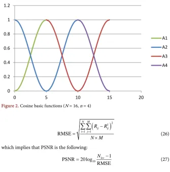
l 1 , l=2,,m−1.

In Figure 2, we show the basic functions (23) for N = 16 and n = 4. The compressed block 1B _{( ) ( )}

kl _{n B} _{m B}

R

×

 

  is decoded to a block ( ) ( )

1B

ij _{N B} _{M B}

R

×

 

 

of sizes N B

( )

×M B

( )

by using the inverse F1-transform defined for every

( ) {

i j, 1,∈ ,N_B

} {

× 1,,M_B

}

as

( ) ( )

( ) ( ) 1

1 1 1

1 1

n B m B B kl k l B k l

ij n B m B

k l

R A i B j

R

A i B j

= =

=

∑ ∑

(25)

which approximates the original block RB_{. Making the union of all the decoded}

blocks R1B_{, we obtain a fuzzy relation (denoted with)}_R1_{of sizes} _N_×_M _{. Then}

(8)

[image:8.595.204.540.66.405.2]

Figure 2. Cosine basic functions (N = 16, n = 4)

(

)

2

1

1 1 RMSE

N M

ij ij i j

R R

N M

= =

− =

×

∑∑

(26) which implies that PSNR is the following:

10 1

PSNR 20 log

RMSE lev N −

= ₍₂₇₎

4. Test Results

We compare our method with the classical F-transform compression method, but here no comparison is made with the one inspired to the Canny method used in [2].

For our tests we have considered the CVG-UGR image database extracting grey images of sizes 256 × 256 (cfr., http://decsai.ugr.es/cvg/dbimagenes/). For brevity, we only give the results for three images as Lena, Einstein and Leopard whose sources are given in Figures 3(a)-(c), respectively.

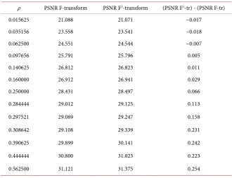
In Table 1, we show the PSNR of the F-transform and F1_{-transform methods}

for some values of the compression rate in the image Lena. We make the following remarks on Table 1:

− for weak compression rates the quality of the decoded image under the F1_{-transform method is better than the one obtained with the F-transform}

method;

− for strong compression rates the quality of the images decoded in the two methods is similar;

− the difference between the two PSNR’s in the two methods overcomes 0.1 for

ρ > 0.25.

In Figure 4, we show the trend of the PSNR for the two methods.

In Figures 5(a)-(d) (resp., Figures 6(a)-(d)), we show the decoded images of Lena obtained by using the F-transform (resp., F1_{-transform) for}_ρ_{= 0.0.0625,}

0.16, 0.284444 and 0.444444, respectively.

0 0.2 0.4 0.6 0.8 1 1.2

0 5 10 15 20

(9)

(a) (b) (c)

[image:9.595.213.534.67.186.2]

Figure 3. (a) Lena; (b) Einstein; (c) Leopard.

Figure 4. PSNR trend for the source image Lena.

Table 1. PSNR of the F-transform and F1_{-transform methods for some values of the}

compression rate in the image Lena.

ρ PSNR F-transform PSNR F1_-transform _{(PSNR F}1_{-tr) - (PSNR F-tr)} 0.015625 21.088 21.071 −0.017

0.035156 23.558 23.541 −0.018 0.062500 24.551 24.544 −0.007 0.097656 25.791 25.796 0.005 0.140625 26.812 26.823 0.011 0.160000 26.912 26.941 0.029 0.250000 28.431 28.497 0.066 0.284444 29.012 29.125 0.113 0.297521 29.089 29.247 0.158 0.308642 29.108 29.339 0.231 0.390625 29.899 30.141 0.242 0.444444 30.800 31.023 0.223 0.562500 31.121 31.375 0.254

20

22

24

26

28

30

32

0

0.2

0.4

0.6 PSN

R

ρ

[image:9.595.209.537.149.422.2] [image:9.595.208.539.484.737.2]

(10)

(a) (b)

(c) (d)

Figure 5. (a) F-tr under ρ = 0.0.0625; (b) F-tr under ρ = 0.16; (c) F-tr decoded (ρ = 0.284444); (d) F-tr decoded (ρ = 0.444444).

(a) (b)

(c) (d)

Figure 6. (a) F1_{-tr decoded (}_ρ_{= 0.0.0625); (b) F}1_{-tr decoded (}_ρ_{= 0.16); (c) F}1_{-tr decoded}

[image:10.595.239.509.66.359.2] [image:10.595.236.512.402.699.2]

(11)

In Table 2 and Figure 7, we show the PSNR obtained using the F-transform and F1_{-transform methods for some values of the compression rate in the image}

Einstein: this table confirms the same results obtained for the image Lena in Ta-ble 1.

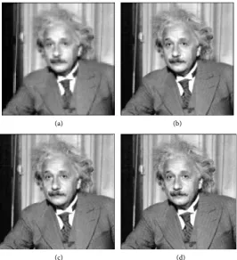
In Figures 8(a)-(d) (resp., Figures 9(a)-(d)) we show the decoded images of Einstein obtained using the F-transform (resp., F1_{-transform) method for}_ρ₌

0.0.0625, 0.16, 0.284444 and 0.444444, respectively.

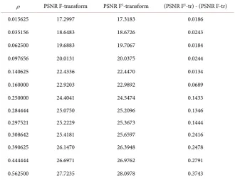
In Table 3 we show the PSNR values obtained using the F-transform and F1_{-transform methods for some values of the compression rate in the image}

[image:11.595.212.537.236.446.2] [image:11.595.208.538.496.739.2]

Leopard.

Figure 7. PSNR trend for the source image Einstein.

Table 2. PSNR results obtained for the source image Einstein.

ρ PSNR F-transform PSNR F1_-transform _{(PSNR F}1_{-tr) - (PSNR F-tr)} 0.015625 22.2701 22.2679 −0.0022 0.035156 23.4968 23.4952 −0.0016 0.062500 24.3781 24.3764 −0.0017 0.097656 25.6269 25.6265 −0.0004 0.140625 26.9260 26.9320 0.0006 0.160000 28.0048 28.0186 0.0138 0.250000 29.3003 29.4154 0.1151 0.284444 30.0018 30.1252 0.1234 0.297521 30.4054 30.5377 0.1323 0.308642 30.5415 30.7242 0.1827 0.390625 31.0126 31.1888 0.1762 0.444444 32.3841 32.6976 0.3135 0.562500 33.2661 33.5678 0.3017

20 22 24 26 28 30 32 34 36

0 0.1 0.2 0.3 0.4 0.5 0.6

PSN

R

ρ

(12)

(a) (b)

(c) (d)

Figure 8. (a) F-tr decoded (ρ = 0.0.0625); (b) F-tr decoded (ρ = 0.16); (c) F-tr decoded (ρ

= 0.284444); (d) F-tr decoded (ρ = 0.444444).

(a) (b)

(c) (d)

[image:12.595.241.506.67.360.2] [image:12.595.241.508.404.697.2]

(13)

Table 3 confirms the results obtained for the images Lena and Einstein: the quality of the decoded image obtained by using the F1_{-transform is better than}

the one obtained using the F-transform for weak compression rates. In Figure 10, we show the trend of the PSNR index obtained by using the two methods.

In Figures 11(a)-(d) (resp., Figures 12(a)-(d)), we show the decoded images of Leopard obtained by using the F-transform (resp., F1_{-transform) method for}_ρ

= 0.0.0625, 0.16, 0.284444, 0.444444, respectively.

[image:13.595.210.534.218.430.2] [image:13.595.209.540.482.735.2]

In Figure 13, we show the trend of the difference of PSNR by varying the compression rate for all the images in the dataset above considered.

Figure 10. PSNR trend for the source image Leopard.

Table 3. PSNR results obtained for the source image Leopard.

ρ PSNR F-transform PSNR F1_-transform _{(PSNR F}1_{-tr) - (PSNR F-tr)} 0.015625 17.2997 17.3183 0.0186

0.035156 18.6483 18.6726 0.0243 0.062500 19.6883 19.7067 0.0184 0.097656 20.0131 20.0375 0.0244 0.140625 22.4336 22.4470 0.0134 0.160000 22.9203 22.9892 0.0689 0.250000 24.4041 24.5474 0.1433 0.284444 25.0750 25.2096 0.1346 0.297521 25.2229 25.3673 0.1444 0.308642 25.4181 25.6597 0.2416 0.390625 26.1470 26.3948 0.2478 0.444444 26.6971 26.9762 0.2791 0.562500 27.7235 28.0978 0.3743

20 21 22 23 24 25 26 27 28 29

0 0.1 0.2 0.3 0.4 0.5 0.6

PSN

R

ρ

(14)

(a) (b)

Figure 11. (a) F-tr decoded (ρ = 0.0.0625); (b) F-tr decoded (ρ = 0.16); (c) F-tr decoded (ρ=0.284444); (d) F-tr decoded (ρ=0.444444).

(a) (b)

[image:14.595.237.510.69.364.2] [image:14.595.238.511.407.698.2]

(15)

[image:15.595.210.540.73.269.2]

Figure 13. PSNR trend for all the images in the dataset considered.

Summarizing, we can say that the presence of the coefficients of the F1_-transform

is negated by noise introduced during the strong compressions, while this effect increases considerably using weak compressions rates.

5. Conclusion

We give an image compression method based on the direct and inverse F1_-transform.

The results show that the PSNR of the reconstructed images with the F1_{-transform-based compression method is better than the one obtained with}

the F-transform-based compression. In the tested dataset of images, we find that the difference between the two corresponding PSNR values is greater than 0.1 (resp., 0.25) for ρ = 0.25 (resp., ρ ≈ 0.5). In the next papers, we shall use the F1_{-transform in data analysis problems.}

Acknowledgements

We also accomplish this research under the auspices of the INDAM-GCNS, Italy. The last author acknowledges a partial support from the European Regional De-velopment Fund in the IT4Innovations Centre of Excellence project (CZ.1.05/ 1.1.00/02.0070).

References

[1] Perfilieva, I. and Hodáková, P. (2013) F1_{-Transform of Functions of Two Variables.} Proceedings of EUSFLAT 2013, Advances in Intelligent Systems Research, Milano, 32, 547-553.

[2] Perfilieva, I., Hodáková, P. and Hurtik, P. (2014) Differentiation by the F-Transform and Application for Edge Detection. Fuzzy Sets and Systems, 288, 96-114.

https://doi.org/10.1016/j.fss.2014.12.013

[3] Perfilieva, I. (2006) Fuzzy Transform: Theory and Application. Fuzzy Sets and Sys-tems, 157, 993-1023.https://doi.org/10.1016/j.fss.2005.11.012

[4] Di Martino, F., Loia, V. and Sessa, S. (2003) A Method in the Compres--0.05

0 0.05 0.1 0.15 0.2 0.25 0.3 0.35

0 0.1 0.2 0.3 0.4 0.5 0.6

F

1 −

F

ρ

(16)

sion/Decompression of Images Using Fuzzy Equations and Fuzzy Similarities. Pro-ceedings of the 10th IFSA World Congress, Istanbul, 30 June-2 July 2003, 524-527. [5] Di Martino, F., Loia, V., Perfilieva, I. and Sessa, S. (2008) An Image

Cod-ing/Decoding Method Based on Direct and Inverse Fuzzy Transforms. International Journal of Approximate Systems, 48, 110-131.

https://doi.org/10.1016/j.ijar.2007.06.008

[6] Di Martino, F. and Sessa, S. (2007) Compression and Decompression of Images with Discrete Fuzzy Transforms. Information Sciences, 177, 2349-2362.

https://doi.org/10.1016/j.ins.2006.12.027

[7] Di Martino, F., Loia, V. and Sessa, S. (2010) A Segmentation Method for Images Compressed by Fuzzy Transforms. Fuzzy Sets and Systems, 161, 56-74.

[8] Di Martino, F., Loia, V. and Sessa, S. (2010) Fuzzy Transforms for Compression and Decompression of Colour Videos. Information Sciences, 180, 3914-3931.

[9] Di Martino, F., Hurlik, P., Perfilieva, I. and Sessa, S. (2014) A Color Image Reduc-tion Based on Fuzzy Transforms. Information Sciences, 266, 101-111.

[10] Di Martino, F. and Sessa, S. (2013) Coding B-Frames on Color Videos with Fuzzy Transforms. Advances on Fuzzy Systems, 2013, Article ID: 652429.

https://doi.org/10.1155/2013/652429

[11] Di Martino, F., Loia, V. and Sessa, S. (2012) Fragile Watermarking Tamper Detec-tion with Images Compressed by Fuzzy Transform. Information Sciences, 195, 62-90. https://doi.org/10.1016/j.ins.2012.01.014

[12] Di Martino, F., Loia, V. and Sessa, S. (2013) Image Matching by Using Fuzzy Transform. Advances on Fuzzy Systems, 2013, Article ID: 760705, 10 p.

[13] Loia, V. and Sessa, S. (2005) Fuzzy Relation Equations for Coding/Decoding Processes of Images and Videos. Information Sciences, 171, 145-172.

[14] Nobuhara, H., Pedrycz, W. and Hirota, K. (2000) Fast Solving Method of Fuzzy Re-lational Equation and Its Application to Lossy Image Compression. IEEE Transac-tions on Fuzzy Systems, 8, 325-334. https://doi.org/10.1109/91.855920

[15] Nobuhara, H., Pedrycz, W. and Hirota, K. (2005) Relational Image Compression: Optimizations through the Design of Fuzzy Coders and YUV Color Space. Soft Computing, 9, 471-479. https://doi.org/10.1007/s00500-004-0366-7

[16] Nobuhara, H., Hirota, K., Di Martino, F., Pedrycz, W. and Sessa, S. (2005) Fuzzy Relation Equations for Compression/Decompression Processes of Colour Images in the RGB and YUV Colour Spaces. Fuzzy Optimization and Decision Making, 4, 235-246. https://doi.org/10.1007/s10700-005-1892-1

[17] Perfilieva, I. and De Baets, B. (2010) Fuzzy Transforms of Monotone Functions with Application to Image Compression. Information Sciences, 180, 3304-3315.

[18] Vajgl, M., Perfilieva, I. and Hodáková, P. (2012) Advanced F-Transform Based Im-age Fusion. Advances in Fuzzy Systems, 2012, Article ID: 125086, 9 p.

https://doi.org/10.1155/2012/125086

[19] Di Martino, F., Loia, V. and Sessa, S. (2010) Fuzzy Transforms Method and Attribute Dependency in Data Analysis. Information Sciences, 180, 493-505.

(17)

[20] Di Martino, F., Loia, V. and Sessa, S. (2011) Fuzzy Transforms Method in Predic-tion Data Analysis. Fuzzy Sets and Systems, 180, 146-163.

[21] Holcapek, M. (2011) A Smoothing Filter Based on Fuzzy Transform. Fuzzy Sets and Systems, 180, 69-97. https://doi.org/10.1016/j.fss.2011.05.028

[22] Perfilieva, I., Novak, V. and Dvorak, A. (2008) Fuzzy Transforms in the Analysis of Data. International Journal of Approximate Reasoning, 40, 26-46.

https://doi.org/10.1016/j.ijar.2007.06.003

[23] Štěpnička, M. and Polakovič, O. (2009) A Neural Network Approach to the Fuzzy Transform. Fuzzy Sets and Systems, 160, 1037-1047.

[24] Štěpnička, M., Dvořák, A., Pavliska, V. and Vavříčková, L. (2011) A Linguistic Ap-proach to Time Series Modeling with the Help of F-Transform. Fuzzy Sets and Sys-tems, 180, 164-184. https://doi.org/10.1016/j.fss.2011.02.017

[25] Troiano, L. and Ktriptani, P. (2011) Supporting Trading Strategies by Inverse Fuzzy Transform. Fuzzy Sets and Systems, 180, 121-145.

[26] Bede, B. and Rudas, I.J. (2011) Approximation Properties of Fuzzy Transforms.

Fuzzy Sets and Systems, 180, 20-40. https://doi.org/10.1016/j.fss.2011.03.001

[27] Perfilieva, I., Dankova, M. and Bede, B. (2011) Towards a Higher Degree F-Transform.

Fuzzy Sets Systems, 180, 3-19.

[28] Di Martino, F., Loia, V. and Sessa, S. (2003) A Method for Coding/Decoding Images by Using Fuzzy Relation Equations. In: Bilgic, T., De Baets, B. and Kaynak, O., Eds.,

Fuzzy Sets and Systems—IFSA 2003, Lecture Notes in Artificial Intelligence, Vol. 2715, Springer, Berlin, 436-441. https://doi.org/10.1007/3-540-44967-1_52

Submit or recommend next manuscript to SCIRP and we will provide best service for you:

Accepting pre-submission inquiries through Email, Facebook, LinkedIn, Twitter, etc. A wide selection of journals (inclusive of 9 subjects, more than 200 journals)

Providing 24-hour high-quality service User-friendly online submission system Fair and swift peer-review system

Efficient typesetting and proofreading procedure

Display of the result of downloads and visits, as well as the number of cited articles Maximum dissemination of your research work

Submit your manuscript at: http://papersubmission.scirp.org/