Self-disclosure topic model for Twitter conversations
JinYeong Bak
Department of Computer Science KAIST
Daejeon, South Korea
Chin-Yew Lin Microsoft Research Asia Beijing 100080, P.R. China
Alice Oh
Department of Computer Science KAIST
Daejeon, South Korea
Abstract
Self-disclosure, the act of revealing one-self to others, is an important social be-havior that contributes positively to inti-macy and social support from others. It is a natural behavior, and social scien-tists have carried out numerous quantita-tive analyses of it through manual tagging and survey questionnaires. Recently, the flood of data from online social networks (OSN) offers a practical way to observe and analyze self-disclosure behavior at an unprecedented scale. The challenge with such analysis is that OSN data come with no annotations, and it would be impos-sible to manually annotate the data for a quantitative analysis of self-disclosure. As a solution, we propose a semi-supervised machine learning approach, using a vari-ant of latent Dirichlet allocation for au-tomatically classifying self-disclosure in a massive dataset of Twitter conversations. For measuring the accuracy of our model, we manually annotate a small subset of our dataset, and we show that our model shows significantly higher accuracy and F-measure than various other methods. With the results our model, we uncover a positive and significant relationship be-tween self-disclosure and online conversa-tion frequency over time.
1 Introduction
Self-disclosure is an important and pervasive so-cial behavior. People disclose personal informa-tion about themselves to improve and maintain relationships (Jourard, 1971; Joinson and Paine, 2007). For example, when two people meet for the first time, they disclose their names and in-terests. One positive outcome of self-disclosure
is social support from others (Wills, 1985; Der-lega et al., 1993), shown also in online social net-works (OSN) such as Twitter (Kim et al., 2012). Receiving social support would then lead the user to be more active on OSN (Steinfield et al., 2008; Trepte and Reinecke, 2013). In this paper, we seek to understand this important social behavior using a large-scale Twitter conversation data, automati-cally classifying the level of self-disclosure using machine learning and correlating the patterns with subsequent OSN usage.
Twitter conversation data, explained in more de-tail in section 4.1, enable a significantly larger scale study of naturally-occurring self-disclosure behavior, compared to traditional social science studies. One challenge of such large scale study, though, remains in the lack of labeled ground-truth data of self-disclosure level. That is, naturally-occurring Twitter conversations do not come tagged with the level of self-disclosure in each conversation. To overcome that challenge, we propose a semi-supervised machine learning approach using probabilistic topic modeling. Our self-disclosure topic model (SDTM) assumes that self-disclosure behavior can be modeled using a combination of simple linguistic features (e.g., pronouns) with automatically discovered seman-tic themes (i.e., topics). For instance, an utterance “I am finally through with this disastrous relation-ship” uses a first-person pronoun and contains a topic about personal relationships.
In comparison with various other models, SDTM shows the highest accuracy, and the result-ing self-disclosure patterns of the users are cor-related significantly with their future OSN usage. Our contributions to the research community in-clude the following:
• We present a topic model that explicitly in-cludes the level of self-disclosure in a conver-sation using linguistic features and the latent semantic topics (Sec. 3).
• We collect a large dataset of Twitter conver-sations over three years and annotate a small subset with self-disclosure level (Sec. 4).
• We compare the classification accuracy of SDTM with other models and show that it performs the best (Sec. 5).
• We correlate the self-disclosure patterns of users and their subsequent OSN usage to show that there is a positive and significant relationship (Sec. 6).
2 Background
In this section, we review literature on the relevant aspects of self-disclosure.
Self-disclosure (SD) level: To quantitatively analyze self-disclosure, researchers categorize self-disclosure language into three levels: G (gen-eral) for no disclosure, Mfor medium disclosure, and H for high disclosure (Vondracek and Von-dracek, 1971; Barak and Gluck-Ofri, 2007). Ut-terances that contain general (non-sensitive) infor-mation about the self or someone close (e.g., a family member) are categorized as M. Examples are personal events, past history, or future plans. Utterances about age, occupation and hobbies are also included. Utterances that contain sensitive in-formation about the self or someone close are cat-egorized asH. Sensitive information includes per-sonal characteristics, problematic behaviors, phys-ical appearance and wishful ideas. Generally, these are thoughts and information that one would generally keep as secrets to himself. All other utterances, those that do not contain information about the self or someone close are categorized asG. Examples include gossip about celebrities or factual discourse about current events.
Classifying self-disclosure level: Prior work on quantitatively analyzing self-disclosure has re-lied on user surveys (Trepte and Reinecke, 2013; Ledbetter et al., 2011) or human annotation (Barak and Gluck-Ofri, 2007). These methods consume much time and effort, so they are not suitable for large-scale studies. In prior work closest to ours, Bak et al. (2012) showed that a topic model can be used to identify self-disclosure, but that work applies a two-step process in which a basic topic model is first applied to find the topics, and then the topics are post-processed for binary classifica-tion of self-disclosure. We improve upon this work by applying a single unified model of topics and
𝑤 𝑧 𝜋
𝑟 𝛼 𝛾
C T N
𝑦
ω
𝜆 𝑥 𝜃𝑙
3
𝛽𝑙
𝜙𝑙
[image:2.595.335.496.62.180.2]𝐾𝑙 3
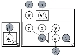
Figure 1: Graphical model of SDTM
self-disclosure for high accuracy in classifying the three levels of self-disclosure.
Self-disclosure and online social network: According to social psychology, when someone discloses about himself, he will receive social sup-port from those around him (Wills, 1985; Derlega et al., 1993), and this pattern of self-disclosure and social support was verified for Twitter con-versation data (Kim et al., 2012). Social support is a major motivation for active usage of social networks services (SNS), and there are findings that show self-disclosure on SNS has a positive longitudinal effect on future SNS use (Trepte and Reinecke, 2013; Ledbetter et al., 2011). While these previous studies focused on small, qualita-tive studies, we conduct a large-scale, machine learning driven study to approach the question of self-disclosure behavior and SNS use.
3 Self-Disclosure Topic Model
This section describes our model, the self-disclosure topic model (SDTM), for classifying self-disclosure level and discovering topics for each self-disclosure level.
3.1 Model
We make two important assumptions based on our observations of the data. First, first-person pro-nouns (I, my, me) are good indicators for medium level of self-disclosure. For example, phrases such as ‘I live’ or ‘My age is’ occur in utterances that re-veal personal information. Second, there are top-ics that occur much more frequently at a particular
SD level. For instance, topics such as physical appearanceandmental healthoccur frequently at levelH, whereas topics such asbirthdayand hob-biesoccur frequently at levelM.
Notation Description
G;M;H {general; medium; high}SDlevel
C;T;N Number of conversations; tweets; words
KG;KM;KH Number of topics for{G; M; H}
c;ct Conversation; tweet in conversationc yct SDlevel of tweetct, G or M/H
rct SDlevel of tweetct, M or H
zct Topic of tweetct
wctn nthword in tweetct
λ Learned Maximum entropy
parame-ters
xct First-person pronouns features
ωct Distribution overSDlevel of tweetct
πc SDlevel proportion of conversationc
θGc;θMc ;θHc Topic proportion of{G; M; H}in
con-versationc
φG;φM;φH Word distribution of{G; M; H} α;γ Dirichlet prior forθ;π βG,βM;βH Dirichlet prior forφG;φM;φH
ncl Number of tweets assignedSDlevell
in conversationc nl
ck Number of tweets assignedSDlevell
and topickin conversationc nl
kv Number of instances of word v
as-signedSDlevelland topick mctkv Number of instances of word v
[image:3.595.73.292.60.351.2]as-signed topickin tweetct
Table 1: Summary of notations used in SDTM.
in it. The first assumption about the first-person pronouns is implemented by the observed variable xct and the parameters λ from a maximum
en-tropy classifier forGvs. M/H level. The second assumption is implemented by the three separate word-topic probability vectors for the three lev-els ofSD: φl which has a Bayesian informative prior βl where l ∈ {G, M, H}, the three levels
of self-disclosure. Table 1 lists the notations used in the model and the generative process, Figure 2 describes the generative process.
3.2 ClassifyingGvsM/Hlevels
Classifying theSDlevel for each tweet is done in two parts, and the first part classifies Gvs. M/H
levels with first-person pronouns (I, my, me). In the graphical model, y is the latent variable that represents this classification, and ω is the distri-bution over y. x is the observation of the first-person pronoun in the tweets, andλare the param-eters learned from the maximum entropy classifier. With the annotated Twitter conversation dataset (described in Section 4.2), we experimented with several classifiers (Decision tree, Naive Bayes) and chose the maximum entropy classifier because it performed the best, similar to other joint topic models (Zhao et al., 2010; Mukherjee et al., 2013).
1. For each levell∈ {G,M,H}: For each topick∈ {1, . . . , Kl}:
Drawφl
k∼Dir(βl)
2. For each conversationc∈ {1, . . . , C}: (a) DrawθG
c ∼Dir(α)
(b) DrawθM
c ∼Dir(α)
(c) DrawθHc ∼Dir(α)
(d) Drawπc∼Dir(γ)
(e) For each messaget∈ {1, . . . , T}:
i. Observe first-person pronouns featuresxct
ii. Drawωct∼MaxEnt(xct,λ)
iii. Drawyct∼Bernoulli(ωct)
iv. Ifyct= 0 which isGlevel:
A. Drawzct∼Mult(θGc)
B. For each wordn∈ {1, . . . , N}: Draw wordwctn∼Mult(φGzct)
Else which can beMorHlevel: A. Drawrct∼Mult(πc)
B. Drawzct∼Mult(θrcct)
C. For each wordn∈ {1, . . . , N}: Draw wordwctn∼Mult(φrzctct)
Figure 2: Generative process of SDTM.
3.3 ClassifyingMvsHlevels
The second part of the classification, theMand the
Hlevel, is driven by informative priors with seed words and seed trigrams.
Utterances with M level include two types: 1) information related with past events and fu-ture plans, and 2) general information about self (Barak and Gluck-Ofri, 2007). For the former, we add as seed trigrams ‘I have been’ and ‘I will’. For the latter, we use seven types of information generally accepted to be personally identifiable in-formation (McCallister, 2010), as listed in the left column of Table 2. To find the appropriate tri-grams for those, we take Twitter conversation data (described in Section 4.1) and look for trigrams that begin with ‘I’ and ‘my’ and occur more than 200 times. We then check each one to see whether it is related with any of the seven types listed in the table. As a result, we find 57 seed trigrams for
Mlevel. Table 2 shows several examples.
Type Trigram
Name My name is, My last name Birthday My birthday is, My birthday party Location I live in, I lived in, I live on
Contact My email address, My phone number Occupation My job is, My new job
[image:3.595.326.503.64.255.2]Education My high school, My college is Family My dad is, My mom is, My family is
Table 2: Example seed trigrams for identifyingM
level ofSD. There are 51 of these used in SDTM.
Category Keywords physical
appearance acne, hair, overweight, stomach, chest,hand, scar, thighs, chubby, head, skinny mental/physical
[image:4.595.77.296.674.751.2]condition addicted, bulimia, doctor, illness, alco-holic, disease, drugs, pills, anorexic
Table 3: Example words for identifyingHlevel of
SD. Categories are hand-labeled.
generally keep as secrests. With this intuition, we crawled 26,523 secret posts from Six Billion Se-crets1site where users post secrets anonymously. To extract seed words that might express secre-tive personal information, we compute mutual in-formation (Manning et al., 2008) with the secret posts and 24,610 randomly selected tweets. We select 1,000 words with high mutual information and filter out stop words. Table 3 shows some of these words. To extract seed trigrams of secretive wishes, we again look for trigrams that start with ‘I’ or ‘my’, occur more than 200 times, and select trigrams of wishful thinking, such as ‘I want to’, and ‘I wish I’. In total, there are 88 seed words and 8 seed trigrams forH.
3.4 Inference
For posterior inference of SDTM, we use col-lapsed Gibbs sampling which integrates out la-tent random variables ω,π,θ, and φ. Then we only need to computey,randz for each tweet. We compute full conditional distributionp(yct = j0, r
ct = l0, zct = k0|y−ct,r−ct,z−ct,w,x) for
tweetctas follows:
p(yct = 0, zct=k0|y−ct,r−ct,z−ct,w,x)
∝ P1exp(λ0·xct)
j=0exp(λj·xct)
g(c, t, l0, k0) p(yct= 1, rct=l0, zct=k0|y−ct,r−ct,z−ct,w,x)
∝ P1exp(λ1·xct)
j=0exp(λj·xct)
(γl0 +n(cl−0ct))g(c, t, l0, k0)
wherez−ct,r−ct,y−ctarez,r,ywithout tweet ct,mctk0(·)is the marginalized sum over wordvof
mctk0v and the functiong(c, t, l0, k0)as follows:
g(c, t, l0, k0) = Γ(
PV
v=1βvl0 +nl
0−(ct)
k0v )
Γ(PVv=1βl0
v +nl
0−(ct)
k0v +mctk0(·))
αk0 +nlck0(0−ct)
PK
k=1αk+nlck0
! V
Y
v=1 Γ(βl0
v +nl
0−(ct)
k0v +mctk0v)
Γ(βl0
v +nl
0−(ct)
k0v )
1http://www.sixbillionsecrets.com
4 Data Collection and Annotation
To answer our research questions, we need a large longitudinal dataset of conversations such that we can analyze the relationship between self-disclosure behavior and conversation frequency over time. We chose to crawl Twitter because it offers a practical and large source of conversations (Ritter et al., 2010). Others have also analyzed Twitter conversations for natural language and so-cial media research (Boyd et al., 2010; Danescu-Niculescu-Mizil et al., 2011), but we collect con-versations from the same set of dyads over several months for a unique longitudinal dataset.
4.1 Collecting Twitter conversations
We define a Twitter conversation as a chain of tweets where two users are consecutively replying to each other’s tweets using the Twitter reply but-ton. We identify dyads of English-tweeting users with at least twenty conversations and collect their tweets. We use an open source tool for detect-ing English tweets2, and to protect users’ privacy, we replace Twitter userid, usernames and url in tweets with random strings. This dataset consists of 101,686 users, 61,451 dyads, 1,956,993 conver-sations and 17,178,638 tweets which were posted between August 2007 to July 2013.
4.2 Annotating self-disclosure level
To measure the accuracy of our model, we ran-domly sample 101 conversations, each with ten or fewer tweets, and ask three judges, fluent in English, to annotate each tweet with the level of self-disclosure. Judges first read and discussed the definitions and examples of self-disclosure level shown in (Barak and Gluck-Ofri, 2007), then they worked separately on a Web-based platform. Inter-rater agreement using Fleiss kappa (Fleiss, 1971) is 0.67.
5 Classification of Self-Disclosure Level This section describes experiments and results of SDTM as well as several other methods for classi-fication of self-disclosure level.
We first start with the annotated dataset in sec-tion 4.2 in which each tweet is annotated withSD
level. We then aggregate all of the tweets of a conversation, and we compute the proportions of tweets in eachSDlevel. When the proportion of
tweets atMorHlevel is equal to or greater than 0.2, we take the level of the larger proportion and as-sign that level to the conversation. When the pro-portions of tweets atMorHlevel are both less than 0.2, we assignGto theSDlevel.
We compare SDTM with the following methods for classifying tweets forSDlevel:
• LDA (Blei et al., 2003): A Bayesian topic model. Each conversation is treated as a doc-ument. Used in previous work (Bak et al., 2012).
• MedLDA (Zhu et al., 2012): A super-vised topic model for document classifica-tion. Each conversation is treated as a doc-ument and response variable can be mapped to aSDlevel.
• LIWC (Tausczik and Pennebaker, 2010): Word counts of particular categories. Used in previous work (Houghton and Joinson, 2012).
• Seed words and trigrams (SEED): Occur-rence of seed words and trigrams which are described in section 3.3.
• ASUM (Jo and Oh, 2011): A joint model of sentiment and topic using seed words. Each sentiment can be mapped to aSDlevel. Used in previous work (Bak et al., 2012).
• First-person pronouns (FirstP): Occurrence of first-person pronouns which are described in section 3.2. To identify first-person pro-nouns, we tagged parts of speech in each tweet with the Twitter POS tagger (Owoputi et al., 2013).
SEED, LIWC, LDA and FirstP cannot be used directly for classification, so we use Maximum en-tropy model with outputs of each of those models as features. We run MedLDA, ASUM and SDTM 20 times each and compute the average accuracies and F-measure for each level. We set 40 topics for LDA, MedLDA and ASUM, 60; 40; 40 top-ics for SDTMKG, KM andKHrespectively, and
setα = γ = 0.1. To incorporate the seed words and trigrams into ASUM and SDTM, we initial-izeβG,βM andβH differently. We assign a high value of 2.0 for each seed word and trigram for that level, and a low value of10−6 for each word
that is a seed word for another level, and a default
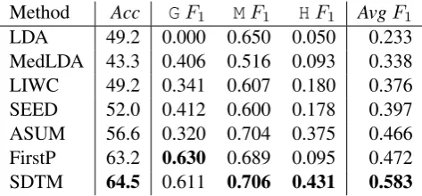
Method Acc GF1 MF1 HF1 AvgF1
[image:5.595.308.545.62.172.2]LDA 49.2 0.000 0.650 0.050 0.233 MedLDA 43.3 0.406 0.516 0.093 0.338 LIWC 49.2 0.341 0.607 0.180 0.376 SEED 52.0 0.412 0.600 0.178 0.397 ASUM 56.6 0.320 0.704 0.375 0.466 FirstP 63.2 0.630 0.689 0.095 0.472 SDTM 64.5 0.611 0.706 0.431 0.583
Table 4:SDlevel classification accuracies and F-measures using annotated data. Acc is accuracy, andGF1 is F-measure for classifying theGlevel. AvgF1 is the average value ofGF1, MF1 andH F1. SDTM outperforms all other methods
com-pared. The difference between SDTM and FirstP is statistically significant (p-value< 0.05 for ac-curacy,<0.0001forAvgF1).
value of 0.01 for all other words. This approach is same as other topic model works (Jo and Oh, 2011; Kim et al., 2013).
As Table 4 shows, SDTM performs better than other methods by accuracy and F-measure. LDA and MedLDA generally show the lowest perfor-mance, which is not surprising given these mod-els are quite general and not tuned specifically for this type of semi-supervised classification task. LIWC and SEED perform better than LDA, but these have quite low F-measure forG andH lev-els. ASUM shows better performance for classi-fyingH level than others, but not for classifying theGlevel. FirstP shows good F-measure for the
G level, but the H level F-measure is quite low, even lower than SEED. Finally, SDTM has sim-ilar performance inGandMlevel with FirstP, but it performs better in H level than others. Classi-fying theHlevel well is important because as we will discuss later, theHlevel has the strongest rela-tionship with longitudinal OSN usage (see Section 6.2), so SDTM is overall the best model for clas-sifying self-disclosure levels.
6 Self-Disclosure and Conversation Frequency
Facebook and StudiVZ users. With SDTM, we can automatically classify self-disclosure level of a large number of conversations, so we investi-gate whether there is a similar relationship be-tween self-disclosure in conversations and subse-quent frequency of conversations with the same partner on Twitter. More specifically, we ask the following two questions:
1. If a dyad displays highSDlevel in their con-versations at a particular time period, would they have more frequent conversations subse-quently?
2. If a dyad shows high conversation frequency at a particular time period, would they dis-play higher SDin their subsequent conver-sations?
6.1 Experiment Setup
We first run SDTM with all of our Twitter con-versation data with 150; 120; 120 topics for SDTM KG, KM and KH respectively. The
hyper-parameters are the same as in section 5. To handle a large dataset, we employ a distributed al-gorithm (Newman et al., 2009).
Table 5 shows some of the topics that were prominent in eachSDlevel by KL-divergence. As expected, Glevel includes general topics such as food, celebrity, soccer and IT devices,Mlevel in-cludes personal communication and birthday, and finally,Hlevel includes sickness and profanity.
For comparing conversation frequencies over time, we divided the conversations into two sets for each dyad. For theinitial period, we include conversations from the dyad’s first conversation to 60 days later. And for the subsequent period, we include conversations during the subsequent 30 days.
We compute proportions of conversation for each SD level for each dyad in the initial and
subsequentperiods. Also, we define a new mea-surement,SDlevel score for a dyad in the period, which is a weighted sum of each conversation with
SDlevels mapped to 1, 2, and 3, for the levelsG,
M, andH, respectively.
6.2 Does self-disclosure lead to more frequent conversations?
We investigate the effect of the level self-disclosure on long-term use of OSN. We run lin-ear regression with the intial SD level score as
1.0 1.5 2.0 2.5 3.0
Initial SD level 1.0
0.5 0.0 0.5 1.0 1.5
[image:6.595.314.519.63.219.2]# Conversaction changes proportion over time
Figure 3: Relationship between initial SD level and conversation frequency changes over time. The solid line is the linear regression line, and the coefficient is 0.118 withp <0.001, which shows a significant positive relationship.
Glevel Mlevel Hlevel Coeff (β) 0.094 0.419 0.464 p-value 0.1042 <0.0001 <0.0001
Table 6: Relationship between initial SD level proportions and changes in conversation fre-quency. For M and H levels, there is significant positive relationship (p < 0.0001), but for theG
level, there is not (p >0.1).
the independent variable, and the rate of change in conversation frequency betweeninitial period andsubsequentperiod as the dependent variable. The result of regression is that the independent variable’s coefficient is 0.118 with a low p-value (p < 0.001). Figure 3 shows the scatter plot with the regression line, and we can see that the slope of regression line is positive.
We also investigate the importance of eachSD
level for changes in conversation frequency. We run linear regression with initial proportions of each SD level as the independent variable, and the same dependent variable as above. As ta-ble 6 shows, there is no significant relationship between the initial proportion of the G level and the changes in conversation frequency (p > 0.1). But for theMandHlevels, the initial proportions show positive and significant relationships with the subsequent changes to the conversation fre-quency (p < 0.0001). These results show thatM
Glevel Mlevel Hlevel
101 184 176 36 104 82 113 33 19
chocolate obama league send twitter going ass better lips butter he’s win email follow party bitch sick kisses
[image:7.595.87.513.62.198.2]good romney game i’ll tumblr weekend fuck feel love cake vote season sent tweet day yo throat smiles peanut right team dm following night shit cold softly milk president cup address account dinner fucking hope hand sugar people city know fb birthday lmao pain eyes cream good arsenal check followers tomorrow shut good neck
Table 5: High ranked topics in each level by comparing KL-divergence with other level’s topics
0 20 40 60 80 100
Initial conversation frequency 1.80
1.85 1.90 1.95 2.00 2.05
Subsequent SD level
Figure 4: Relationship between initial conversa-tion frequency and subsequent SD level. The solid line is the linear regression line, and the co-efficient is0.0016withp <0.0001, which shows a significant positive relationship.
6.3 Does high frequency of conversation lead to more self-disclosure?
Now we investigate whether theinitial conversa-tion frequency is correlated with theSDlevel in thesubsequentperiod. We run linear regression with the initial conversation frequency as the inde-pendent variable, andSDlevel in the subsequent period as the dependent variable.
The regression coefficient is0.0016with low p-value (p < 0.0001). Figure 4 shows the scatter plot. We can see that the slope of the regression line is positive. This result supports previous re-sults in social psychology (Leung, 2002) that fre-quency of instant chat program ICQ and session time were correlated to depth of SD in message.
7 Conclusion and Future Work
In this paper, we have presented the self-disclosure topic model (SDTM) for discovering topics and
classifying SD levels from Twitter conversation data. We devised a set of effective seed words and trigrams, mined from a dataset of secrets. We also annotated Twitter conversations to make a ground-truth dataset for SD level. With annotated data, we showed that SDTM outperforms previous methods in classification accuracy and F-measure.
We also analyzed the relationship between SD level and conversation frequency over time. We found that there is a positive correlation between initial SD level and subsequent conversation fre-quency. Also, dyads show higher level of SD if they initially display high conversation frequency. These results support previous results in social psychology research with more robust results from a large-scale dataset, and show importance of looking at SD behavior in OSN.
There are several future directions for this re-search. First, we can improve our modeling for higher accuracy and better interpretability. For instance, SDTM only considers first-person pro-nouns and topics. Naturally, there are patterns that can be identified by humans but not captured by pronouns and topics. Second, the number of topics for each level is varied, and so we can explore nonparametric topic models (Teh et al., 2006) which infer the number of topics from the data. Third, we can look at the relationship be-tween self-disclosure behavior and general online social network usage beyond conversations.
Acknowledgments
[image:7.595.81.282.243.397.2]References
JinYeong Bak, Suin Kim, and Alice Oh. 2012. Self-disclosure and relationship strength in twitter con-versations. InProceedings of ACL.
Azy Barak and Orit Gluck-Ofri. 2007. Degree and reciprocity of self-disclosure in online forums.
Cy-berPsychology & Behavior, 10(3):407–417.
David M Blei, Andrew Y Ng, and Michael I Jordan. 2003. Latent dirichlet allocation. Journal of
Ma-chine Learning Research, 3:993–1022.
Danah Boyd, Scott Golder, and Gilad Lotan. 2010. Tweet, tweet, retweet: Conversational aspects of retweeting on twitter. InProceedings of HICSS. Cristian Danescu-Niculescu-Mizil, Michael Gamon,
and Susan Dumais. 2011. Mark my words!: Lin-guistic style accommodation in social media. In
Proceedings of WWW.
Valerian J. Derlega, Sandra Metts, Sandra Petronio, and Stephen T. Margulis. 1993. Self-Disclosure, volume 5 of SAGE Series on Close Relationships. SAGE Publications, Inc.
Joseph L Fleiss. 1971. Measuring nominal scale agreement among many raters. Psychological
bul-letin, 76(5):378.
David J Houghton and Adam N Joinson. 2012. Linguistic markers of secrets and sensitive self-disclosure in twitter. InProceedings of HICSS.
Yohan Jo and Alice H Oh. 2011. Aspect and senti-ment unification model for online review analysis.
InProceedings of WSDM.
Adam N Joinson and Carina B Paine. 2007. Self-disclosure, privacy and the internet. The Oxford
handbook of Internet psychology, pages 237–252.
Sidney M Jourard. 1971. Self-disclosure: An experi-mental analysis of the transparent self.
Suin Kim, JinYeong Bak, and Alice Haeyun Oh. 2012. Do you feel what i feel? social aspects of emotions in twitter conversations. InProceedings of ICWSM.
Suin Kim, Jianwen Zhang, Zheng Chen, Alice Oh, and Shixia Liu. 2013. A hierarchical aspect-sentiment model for online reviews. InProceedings of AAAI.
Andrew M Ledbetter, Joseph P Mazer, Jocelyn M DeG-root, Kevin R Meyer, Yuping Mao, and Brian Swaf-ford. 2011. Attitudes toward online social con-nection and self-disclosure as predictors of facebook communication and relational closeness.
Communi-cation Research, 38(1):27–53.
Louis Leung. 2002. Loneliness, self-disclosure, and icq (” i seek you”) use. CyberPsychology & Behav-ior, 5(3):241–251.
Christopher D Manning, Prabhakar Raghavan, and Hinrich Sch¨utze. 2008. Introduction to information
retrieval, volume 1. Cambridge University Press
Cambridge.
Erika McCallister. 2010.Guide to protecting the
confi-dentiality of personally identifiable information.
DI-ANE Publishing.
Arjun Mukherjee, Vivek Venkataraman, Bing Liu, and Sharon Meraz. 2013. Public dialogue: Analysis of tolerance in online discussions. InProceedings of
ACL.
David Newman, Arthur Asuncion, Padhraic Smyth, and Max Welling. 2009. Distributed algorithms for topic models. Journal of Machine Learning
Re-search, 10:1801–1828.
Olutobi Owoputi, Brendan OConnor, Chris Dyer, Kevin Gimpel, Nathan Schneider, and Noah A Smith. 2013. Improved part-of-speech tagging for online conversational text with word clusters. In
Proceedings of HLT-NAACL.
Alan Ritter, Colin Cherry, and Bill Dolan. 2010. Unsu-pervised modeling of twitter conversations. In
Pro-ceedings of HLT-NAACL.
Charles Steinfield, Nicole B Ellison, and Cliff Lampe. 2008. Social capital, self-esteem, and use of on-line social network sites: A longitudinal
analy-sis. Journal of Applied Developmental Psychology,
29(6):434–445.
Yla R Tausczik and James W Pennebaker. 2010. The psychological meaning of words: Liwc and comput-erized text analysis methods. Journal of Language
and Social Psychology.
Yee Whye Teh, Michael I Jordan, Matthew J Beal, and David M Blei. 2006. Hierarchical dirichlet pro-cesses. Journal of the american statistical
associ-ation, 101(476).
Sabine Trepte and Leonard Reinecke. 2013. The re-ciprocal effects of social network site use and the disposition for self-disclosure: A longitudinal study.
Computers in Human Behavior, 29(3):1102 – 1112.
Sarah I Vondracek and Fred W Vondracek. 1971. The manipulation and measurement of self-disclosure in preadolescents.Merrill-Palmer Quarterly of
Behav-ior and Development, 17(1):51–58.
Thomas Ashby Wills. 1985. Supportive functions of interpersonal relationships. Social support and
health, xvii:61–82.
Wayne Xin Zhao, Jing Jiang, Hongfei Yan, and Xiaom-ing Li. 2010. Jointly modelXiaom-ing aspects and opin-ions with a maxent-lda hybrid. In Proceedings of
EMNLP.
Jun Zhu, Amr Ahmed, and Eric P Xing. 2012. Medlda: maximum margin supervised topic models. Journal