Data Compression using Simulated Circular Indexing Transform (SCIT)

Data Compression using Simulated Circular Indexing

Transform (SCIT)

Gebremichael Girmay

D. Lalitha Bhaskari

Andhra University College of Engineering (A), Andhra University, Visakhapatnam-530003, India

ABSTRACT

One of the critical issues in big data environment is the volume of the data generated and streamed in real time or archived for later use. If the data streamed in real-time is large enough then the time required to transmit that data may lead to unnecessary delay and latency problems. The other case with huge volumes of data when it is archived is the case of storage devices requirements. Com-pressing the data before or while transmitting is one useful solu-tion to minimize the size of data and thus avoid or minimize the latency problem and storage shortages. In this research paper the focus will be to deal on some compression techniques, especially in data transforming techniques similar to BWT, MTF and RLE which are commonly used to transform the data prior to encoding the data into fewer bits using entropy encoding techniques such as Huffman, Arithmetic, Golomb, etc. All the data transforming techniques have their own positive and weak sides. Thus in this paper alternative method is proposed to fill some of the gaps that cannot be solved by the already existing data compression trans-forming techniques. The proposed algorithm can be combined with other data compression methods to optimize the compression effi-ciency. The performance of this proposed algorithm is measured as compared to other related compression algorithms, and it is found that in some special cases it can perform better than others.

General Terms

Data compression, transforming, modeling, entropy encoding, lossless and lossy, statistical, dictionary, performance, big data.

Keywords

Info-table, unique symbol, codeword, SCIT, frequency, gap, critical issue.

1. INTRODUCTION

Data compression is the process of minimizing the size of code generated by digital coding systems to represent a specific data or information. Digital coding is the process of using binary digits or bits to represent letters, characters and other symbols in a digital format. A digital system is a device or technology that generates discrete values based on some bit combination techniques, so that each character, letter or symbol is unique and easily distinguish-able from each ones. There are several types of digital coding tech-niques widely used, which include ASCII code, BCD/EBCDIC,

UNICODE, etc. For example, using ASCII code, a digital system can generate 128 unique symbols, while using EBCDIC it can pro-vide 256 unique symbols.

In this paper, the necessity and advantage of compression is dis-cussed based on data transfer and data storage issues, and some well-known compression algorithms and techniques are reviewed in brief.

As stated in [1], data compression is the process of converting an input data stream (the source stream or the original raw data) into another data stream (the output, or the compressed, stream) that has a smaller size.

One of the necessities for choosing to compress data is to mini-mize transfer delay/latency during data communication using any media. Specifically, if the input data is generated in real time and is streamed on the way or is stored in memory and is to be trans-ferred to any other destination at any time using speed-constrained systems.

The second issue is when there is small storage volume within the system, but the data or document is to be archived for later use. Other issues are such as to speed up the data processing operations, to reduce energy required to process or to transmit, and for security purposes as well.

Data compression works if the original file of data is re-encoded as follows:

- Reduce the number of symbols in the data using predictive meth-ods.

- Rearrange the symbols in the data using transform techniques. - Encode more frequent symbols with fewer bits.

RLE is an example of compression technique that works well on documents that exhibit to contain repetitive symbols. BWT, MTF, PPM, and Differencing are some examples of predictive/transform techniques used to rearrange characters or symbols within a docu-ment after which it is possible to more reduce the size of the doc-ument. Huffman coding, Arithmetic coding, Shannon-Fano, Tun-stall, Elias gamma, and other more methods are those used to en-code frequent symbols with fewer bits.

the original data but an approximation that is somewhat similar to the original version. Lossy compression is useful when compress-ing pictures (e.g., JPEG) or audio files (e.g., MP3), where small deviations from the original are invisible (or inaudible) to the hu-man senses [2].

Codes can be categorized as block-block, block-variable, variable-block, or variable-variable [3]. Compression coding techniques such as Huffman and Arithmetic generate variable-length code-word for every unique symbol or group of symbols. Coding meth-ods such as ASCII generate fixed-length codes for every unique character.

In this paper we focus exclusively on lossless compression algo-rithms, by modeling and implementing a new transform technique similar to MTF method and encoding using Huffman coding as a final step.

Most compression/decompression systems apply a combination of several techniques to achieve better compression efficiency. Com-pression/decompression performance is measured based on the data type compressed, and whether it is lossy or lossless compres-sion. Commonly used performance measurement methodologies include: compression ratio, compression factor, compression gain, compression rate, and fidelity. In most cases, if possible, the goal is to achieve a best compression factor and speed with less degrad-ing fidelity; Entropy bedegrad-ing a reference for better encoddegrad-ing factor, as defined by Shannon.

In subsequent sections and subsections, the basic concepts of com-pression will be covered in some detail. Section 2, literature review, Section 3, modeling and coding and Section 4, proposed technique and its implementation will be covered.

2. LTITERATURE REVIEW

The research works done in the compression/decompression area is wide, and is still continuing in several fields as the data generated is vastly growing at high rate. In this chapter some basic theoreti-cal and practitheoreti-cal concepts and approaches are reviewed. Generally compression can be lossless or lossy. Lossless compression is con-cerned with textual documents and some critical data such as med-ical scanning images. Lossless data compression methods can be classified as Entropy type, Dictionary type, and other types [1].

In entropy (or statistical) coding each symbol is assigned a code based on the probability model that is chosen. Highly probable symbols are assigned short codes, and vice versa. In dictionary coding, groups of consecutive characters, words, or phrases are re-placed with seemingly short code. The group of symbols or words represented by the corresponding codes can be found by referring it in the dictionary.

Lossy data compression goes with general images, videos and au-dios. Next some commonly used optimal encoding algorithms are detailed, tuning towards the proposed method. Indeed saving stor-age space is a common reason for the use of compression [4], and other reasons are of course speed and band width utilization.

2.1 Huffman Coding

Huffman coding, developed, in 1952, by D. Huffman, is a popular method for data compression, categorized under the entropy coders. An entropy coder is a method that assigns to every symbol from the alphabet a code depending on the probability of symbol occurrence [5]. The symbols that are more probable to occur get shorter codes

than the less probable ones. Huffman coding is an optimal coding technique for compression purpose and serves as the basis for sev-eral popular programs run on various platforms [6]. Some programs use just the Huffman method, while others use it as one step in a multistep compression process. The Huffman method is somewhat similar to the Shannon-Fano method. Huffman coding is one of the best methods for coding with respect to probabilistic model.

Though the size of the code assigned to a symbolaibasically de-pends on its probability of occurrencespiit is also affected by the number of unique symbols (the size of the alphabet) in the stream or document. A small alphabet requires just a few codes, so they can all be short; a large alphabet requires many codes, so some must be long. One critical issue in Huffman coding is that, if those unique symbols (whether they are few or more) that constitute a given data file, do appear with equal probabilities (or frequency of occur-rence), it may not considerably change the size of the document. For example, if there arenunique symbols andn= 2m_{, wherem} is a common code length (e.g. for ASCII code,m= 7, n= 128) supported by the system when generating each alphanumeric char-acters and symbols, applying Huffman coding will not affect the original size of the document. Thus in such related cases some transform or predictive techniques are required either to:

- reduce the number of unique symbols, or

- vary the frequency of the representative symbols, or

- rearrange their position in the document so that produce a repet-itive form.

What it means is, the Huffman method cannot assign to any sym-bol a code shorter than one bit, if some form of predictive transform is not done ahead to using Huffman coding. Therefore to achieve meaningful compression process, a need comes to apply a multistep compression process, the last step being Huffman or other statisti-cal coding methods such us Arithmetic, Elias, Golomb, and more others. The multistep compression process may incorporate RLE, BWT, MTF, and PPM, etc. compression techniques that can be ap-plied prior to conducting Huffman or the other statistical coding methods.

Huffman Decoding:During compressing some basic information must be collected in the form of Information Table (Info-table). These points (info) include: list of the unique symbols and their probability (or frequency); and if required, their variable-size code-word, the size of the original and compressed file. During decod-ing the compressor (encoder) has to determine the codes based on the supplied points in the info-table. Basically it does that based on the probabilities (or frequencies of occurrence) of the symbols. The Huffman decompressor (decoder) must first construct (map) the Huffman tree as was constructed by the compressor (encoder). Only then can it read and decode the compressed stream. Then, if a multistep compression was used, the decompressor should follow the same step but in reverse order, to gate the original stream.

2.2 Run Length Encoding (RLE)

It replaces a run of symbols with a tuple that contains the sym-bol and the number of times it is repeated [7]. In general, a string

s1s1...s1s2s2...s2s3s3..., in which each symbol appears in a long run (as countable infinite repetitive) is suitable to reduce the runs and thus reducing(compressing) the size of the string. Example, the string ”ssssiiiiooonn” can be encoded or transformed using RLE as 4s4i3o2n. Then it can further be coded using statistical models such as Huffman or Arithmetic encoders.

One of the critical issues in using RLE is when the similarity run of symbols is short (e.g. one or two), which will result in increasing the size rather than compressing it. Anyway, RLE can be used at the beginning or after some techniques are processed in most multistep compression process, e.g., RLE–BWT–MTF–RLE–Huffman [8].

2.3 Move-to-Front Transform

Move-to-Front (MTF) is an adaptive scheme and works on the prin-ciple that the appearance of a symbol in the input data makes that symbol more likely to appear in the near future. As detailed in [9] the basic idea of this method is to maintain the alphabetAof sym-bols as a list where frequently-occurring symsym-bols are located near the front. A symbols is encoded as the number of symbols that precede it in this list. Thus if alphabetA= (C, o, m, p, r, e, s, . . .) and the next symbol in the input stream to be encoded is thep, it will be encoded as 3, since it is preceded by three symbols. There are several possible variants to this method; the most basic of them adds one more step: After symbolsis encoded, it is moved to the front of listA. Thus, after encoding thep, the alphabet is modified toA= (p, C, o, m, r, e, s, . . .). This move-to-front step reflects the expectation that oncephas been read from the input stream, it will be read many more times and will, at least for a while, be a com-mon symbol. The move-to-front method is locally adaptive, since it adapts itself to the frequencies of symbols in local areas of the input stream. The main idea is to move to front the symbols that mostly occur, so those symbols will have smaller output number or results in to more repetitiveness and thus will be coded with short codeword bits. Example, as the input document is processed, each symbol (or word, when used at world level) is looked up in the al-phabet list and if it happens to occur as theith_{entry, it is coded by} the index numberi. Then the symbol is moved to the front of the list so that if it occurs soon afterwards, it will be coded by a number smaller thani.

This technique is intended to be used in combination with other compression techniques like Burrows-wheeler transform (BWT).

After a stream is transformed using MTF, then follows encod-ing it usencod-ing either of the variable length entropy encoders such as Golomb, Huffman, arithmetic, etc.

An optional example is the numberiis coded so that the smaller its value the shorter its code, and thus more likely symbols are repre-sented more compactly.For instance, one suitable method of assign-ing variable code lengths is to code position index integer number

i≥ 1as the binary representation ofiprefixed byblogi 2czeros. In this case as the binary code of the integeriis1 +blogi₂cbits long, then addingblogi2czeros becomes1 + 2blog

i

2cbits [1]. For example the codes foriis 1, 2, 3, and 4 are 1, 010, 011, and 00100, respectively.

Therefore this method produces good results if the input stream contains concentrations of identical symbols, i.e. if the stream sat-isfies the concentration property (if the local frequency of symbols changes significantly from area to area in the input stream).

It can be shown that the move-to-front method performs, in the worst case, slightly worse than Huffman coding. At best, it per-forms significantly better when it is used with BWT or when the frequencies of the symbols in the input file are or not varied mean-ingfully, but appearing repetitively.

There are several possible variants to this

method:-Move-ahead-k- The element ofAmatched by the current symbol is moved aheadkpositions instead of all the way to the front ofA.

Wait-c-and-move- An element ofAis moved to the front only after it has been matchedctimes to symbols from the input stream (not necessarilycconsecutive times).

A critical issue in using MTF is, it gives poor performance if re-quest sequence is in reverse order of the alphabet list [10]. That is if the distribution of the symbols in the stream appears in reverse order at seemingly equal interval, then using MTF will not achieve good compression performance.

2.4 Burrows-Wheeler-Transform (BWT)

As explained in [9, 11], BWT method was developed by Michael Burrows and David Wheeler in 1994, while working at DEC Sys-tems Research Centre in Palo Alto, California. The main idea of the BWT method is that it starts with a stringSofmsymbols and scramble (permute) them into another stringL that satisfies two conditions.

(1) Any region of Lwill tend to have a concentration of just a few symbols. Another way of saying this is if a symbolsis found at a certain position inL, then other occurrences ofs

are likely to be found nearby. This property means thatLcan easily and efficiently be compressed with the move-to-front method, perhaps in combination with RLE and then apply a statistical model(e.g. Huffman or others) to assign probabili-ties to the transformed symbols.

(2) It is possible to reconstruct the original stringSfromL(a little more data may be needed for the reconstruction, in addition to

L, but not much).

One of the critical issues is that, the BWT method will work well only ifmis large (at least several thousand symbols per string) [9]. Another case is that, as a string withmsymbols can havem! per-mutations, it becomes a large number for large value ofm, thus the particular permutation used by BWT has to be carefully selected.

The BW codec proceeds in the following steps:

(1) StringL is created, by the encoder, as a permutation ofS. Some more information, denoted byI, is also created, to be used later by the decoder in step 3.

(2) The encoder compressesLandIand writes the results on the output stream. This step typically starts with RLE, continues with move-to-front coding, and finally applies Huffman cod-ing.

(3) The decoder reads the output stream and decodes it by applying the same methods as in 2 above but in reverse order. The result is stringLand variableI.

(4) BothLandIare used by the decoder to reconstruct the original stringS.

Given an input string ofmsymbols, the encoder constructs anm×

mmatrix where it stores stringSin the top row, followed by(m−

The permutationLselected by the encoder is the last column of the sorted matrix. It should be noted that the Burrows-Wheeler method can easily achieve efficient compression when applied to longer strings (thousands of symbols), though it requires more memory and time to do that. Thus WBT works in block wise.

2.5 Entropy

Entropy is one of the important concepts in information theory. It is a theoretical measure of quantity of information [5, 6, 7, 9, 12]. Entropy is a measure of the amount of order or redundancy in a message. The value of entropy is small if there is a lot of order and otherwise it is large if there is a lot of disorder. Entropy as a mea-sure is very important with regard to achieving better data compres-sion goals, because the length of a message after it is compressed (encoded) should ideally be equal to its entropy. That is entropy gives an estimate of how long to make the encoded version of each symbol in a massage.

As Shannon demonstrated, for a set of possible events with known probabilitiesp1, p2, p3, . . . , pn, that sum to 1, the Entropy of these events is given as

E(p1, p2, p3, . . . , pn) =−k n X

i=1

pilogp2i

where, the positive constantkgoverns the units in which entropy is measured. As normally, the units are bits, wherek=1, and logs are taken with base 2, then:

E=−

n X

i=1

pilog pi

2

The information content or entropy of a selected probabilitypiis thus given as

Ei=−pilog pi

2

From this it is clear that more likely symbols or messages having greater probabilities contain less information.

3. MODELING AND CODING

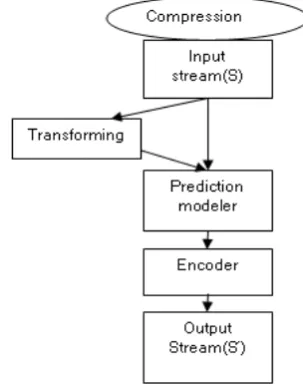
The task of finding a suitable model for text compression is an ex-tremely important problem. As shown in Figure 1, some basic steps are conducted to reach the final compression step. The input mes-sage can be transformed first ahead to applying prediction. The sep-aration into modeller and encoder is valuable because modeling and coding are very different sorts of activity [4]. The modeller deter-mines the probability of the unique symbols in the text and supplies to the encoder. Once prediction is applied, the encoder receives the predicted probability or frequency of occurrences together with the actual input stream and turns them into sequence of bits (binary digits) to be transmitted or saved.

There are three ways that the encoder and the decoder can maintain the same model: static, semi-adaptive, adaptive modeling.

In general in statistical compression process the stream can be first transformed so by doing that the size of the stream and/or the num-ber of unique symbols can be minimized or their frequency can be more skewed as is observed in RLE, BWT, MTF, etc. This paper work is also focusing on the transforming part of the statistical en-coding.

Text Compression:

As mentioned in the previous sections some context-based text

Fig. 1. Outline of Basic Steps in Lossless Compression

compression methods perform a transformation on the input data and then apply a statistical model to assign probabilities to the transformed symbols. Good examples of such methods are the Burrows-Wheeler method, also known as the Burrows-Wheeler transform.

Most text compression methods are either statistical or dictionary based [9, 13]. In dictionary based method the text is fragmented into words and is saved in a data structure called a dictionary. When a fragment of new text is found to be identical to one of the dic-tionary entries, a pointer or a symbol that identify to that entry is written on the compressed stream, to become the compression of the new fragment. In statistical method, on the other hand, consists of methods that develop statistical models of the text as discussed above. The model can be static or dynamic (adaptive). A static model uses fixed probabilities, whereas a dynamic model modifies the probabilities on the fly while text is being input and compressed. Most models are based on one of two approaches: Frequency and Context. In context-based model, the modeller considers the con-text of a symbol when assigning it a probability. Since the decoder does not have access to future text, both encoder and decoder must limit the context to past text, i.e., to symbols that have already been input and processed.

4. PROPOSED METHOD: SIMULATED

CIRCULAR INDEXING TRANSFORM (SCIT)

If the probabilities of the symbols in a document are more skewed, then applying statistical coding methods directly can achieve good results. The fact that the probability is skewed implies low entropy which in turn implies the possibility of very good compression.

repetitively. Conceptually all the moves (next/back or up/down) are mapped or simulated circularly to the position index value of the symbols in the alphabet, except that don‘t move or ‘stay there‘ case is given a 0 index value for a repetitive symbol.

In move-to-front and some other transforming methods, the trans-formed data is represented by the indexes (numerical values). In the proposed SCIT method, the index is translated to the symbol cur-rently indexed, thus the transformed data is represented by the sym-bol themselves. As this translated (virtual) indexing works right, for comparison and compatibility purpose, the MTF is also imple-mented using this concept in this work. For example take the input string is:

S:Compression is very important.

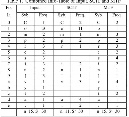
Here,S = 30 characters, and the unique symbols or alphabets aren= 15as seen in the info-table: Info-table basically contains

P0, Ia→

0 1 2 3 4 5 6 7 8 9 a b c d e

C o m p r e s i n ↑ v y t a .

unique symbols in S and may include their codeword and some ad-ditional information, such as frequencies of each unique symbol. Let use these variables:n, Ia, P v, P0; where

n-total number of unique symbols in the streamS.

Ia-holds the index value of a next symbol to be accessed, in the infotable.

P v-virtual(simulated) index, in terms of numeric or the symbols themselves.

P0-actual index value of immediate previously accessed symbol.

Now, we can formulate the proposed method as follows. Initially

Ia, P v, andP0are assigned to a specific value, example 0 index values.

a) During encoding:For each byte in the stream find correspond-ingP vas follows.

P v=Ia−P0, ifIa≥P0; otherwise,P v= (n+Ia)−P0, ifIa < P0.

P0 = (P v+P0)mod(n)

Example,

Ia→

S:C o m p r e s s i o n↑i s↑v e r y↑i m p o r t a n t . = 30(15)

Pv:0 1 1 1 1 1 1 0 1 9 7 1 d e 3 1 a e 7 d d a 1 d 3 8 1 a 4 2 = 30(11)

P0:0 1 2 3 4 5 6 6 7 1 8 9 7 6 9 a 5 4 b 9 7 2 3 1 4 c d 8 c e Or,P vis represented by the name of the symbols themselves in-stead of using numeric values (Note: Here, vertical arrow↑replaces space),

Pv:C o o o o o o C o↑i o a . p o v . i a a v o a p n o v r m = 30(11) RepresentingP vin this way avoids writing two or more digit index values. The successive list ofP vgives the transformed variant of thatS. The value 0 in theP vlist is to mean don‘t move, that means take the current symbol, rather. Since, a pointer at starting time, in most cases, points to the first byte/word in an input stream or document, the first 0 inP vtells to consider the first character inS

which in this illustration is, C character.

Now as a last step is to codeP vlist (transformed stream,S‘) using either Huffman or other statistical coding techniques. This encoded

or compressed document as well including the info-table is then to be communicated or archived as was intended.

Note that the number inside the parenthesis, e.g., 15 in 30(15), 11 in 30(11) represents the number of unique symbols in the original and transformed strings respectively.

b) During decoding:Huffman or other coded doc is decoded or decompressed to obtainP vlist back. Then retransformP vlist to get backS, as follows.

First translate eachP velement or symbol to corresponding nu-meric value one at a time.

Next determine the corresponding actual indexIa orP0and refer the symbol at that location in the info-table and formSin sequence character by character.

P0 = (P v+P0)mod(n),Ia←P0

Example,

Pv:C o o o o o o C o↑i o a . p o v . i a a v o a p n o v r m = 30(11)

Pv:0 1 1 . . .

P0:0 1 2 . . .

Ia→

S:C o m p r e s s i o n↑i s↑v e r y↑i m p o r t a n t . = 30(15) For the above transforming and retransforming example, Move-to-Front, will do as follows.

Ia→

S:C o m p r e s s i o n↑i s↑v e r y↑i m p o r t a n t . = 30(15)

Pv:0 1 2 3 4 5 6 0 7 6 8 9 3 4 2 a 6 7 b 4 6 a a a 6 c d c 2 e = 30(15) i.e., using the symbols instead,

Pv:C o m p r e s C i e n↑p r m v s i y r s v v v s t a t m . = 30(15) We can see that the number of unique symbols after transforming using the SCIT method is 11 while after using MTF is 15 same as in the original document.

As is observed in the info-table, Table 1, the transformed string may have less number of unique symbols (Syb.) as compared to the original string. This phenomenon holds true also for MTF in other examples. And also some of the symbols will gain highest frequency (Freq.) though in some cases, the SCIT technique propa-gates and equalizes the frequency for many symbols in which case the performance will decrease. Now when we apply the statistical encoding technique, Huffman coding, then,

S→115 bits≈15bytes/30; if Huffman(HM) is solely used.

MTF: S’→111 bits≈14bytes/30; if MTF→HM multistep is used.

SCIT: S’→91 bits≈12bytes/30; if SCIT→HM multistep is used.

Observations:

(1) Using Huffman without using SCIT or MTF methods perform optimally in most normal texts or cases.

(2) Using MTF in combination with BWT performs better than Huffman in many cases. i.e., BWT→MTF→Huffman (3) Using SCIT method with or without BWT performs better than

Huffman and MTF for special cases only. SCIT→Huffman or BWT→SCIT→Huffman

Let examine more examples that are special cases:

S1:aabbbccddeefffgghh =18(8)bytes

Huffman:→54bits≈7bytes/18

MTF:aabaacadaeafaagaha =18(8)bytes→38bits≈5bytes/18

Table 1. Combined Info-Table of Input, SCIT and MTF

Po, Input SCIT MTF

Ia Syb. Freq. Syb. Freq. Syb. Freq.

0 C 1 C 2 C 2

1 o 3 o 11 o 1

2 m 2 m 1 m 3

3 p 2 p 2 p 2

4 r 3 r 1 r 3

5 e 2 e 2

6 s 3 s 4

7 i 3 i 2 i 2

8 n 2 n 1 n 1

9 ↑ 3 ↑ 1 ↑ 1

a v 1 v 3 v 4

b y 1 y 1

c t 2 t 2

d a 1 a 4 a 1

e . 1 . 2 . 1

n=15, S =30 n=11, S‘=30 n=15, S‘=30

S2: abcdefghijklmnopqrstuvwxyzzyxwvutsrqponmlkjihgfedcba =52(26) bytes

Huffman:→248bits≈31 bytes/52

MTF:abcdefghijklmnopqrstuvwxyzabcdefghijklmnopqrstuvwxyz =52(26) bytes→248bits≈31 bytes/52

SCIT: abbbbbbbbbbbbbbbbbbbbbbbbbazzzzzzzzzzzzzzzzzzzzzz zzz =52(3) bytes→79bits≈10 bytes/52

S3: abcdefghijklmnopqrstuvwxyzabcdefghijklmnopqrstuvwxyz =52(26) bytes

Huffman:→248bits 31 bytes/52

MTF: abcdefghijklmnopqrstuvwxyzzzzzzzzzzzzzzzzzzzzzzzzzzz =52(26) bytes→170bits≈22 bytes/52

SCIT:abbbbbbbbbbbbbbbbbbbbbbbbbbbbbbbbbbbbbbbbbbbbbbb bbbb =52(2) bytes→52bits≈7 bytes/52

(Now if we apply more methods such as RLE just after applying SCIT, the compressed document may come down to less than 5 bytes only.)

In this last example, S3, though unique symbols in MTF seem more as compared to SCIT, the difference in the compressed outcome is just 15 bytes even though S3 can repeat million times in that sim-ilarity and repetitive sense of sequence. But in the first and second examples SCIT performs best as compared with Huffman alone or MTF.

5. RESULTS & PERFORMANCE COMPARISON

The amount of compression that can be obtained using current tech-niques is in most cases a trade-off against speed and the amount of memory required. Here to evaluate the performance of the proposed transforming technique, SCIT, it is compared with MTF with and without using BWT. Especially a focus is given for the cases that the proposed technique can achieve better performance.

Commonly used benchmark test files can be found from the Cal-gary and Canterbury Corpus which includes text, image, and object files that can be used to evaluate lossless compression methods. Thus using some of this files and additional files it is to be demon-strated that the SCIT techniques will work better for some special arrangement or distribution of symbols in particular files.

Some of the basic points assumed to measure compression are memory required to implement the method, how speedy the method performs on a given system, the amount of compression gained, how closely the reconstruction resembles the original stream (fi-delity), and the relative complexity of the algorithm. Out of these measuring factors memory and time efficiency are the main to be considered [14, 15].

- Compression-ratio, CR=Size of the compressed stream_{Size of the input stream}

- Compression-factor, CF=1 x=

Size of the input stream size of the compressed stream - Compression-gain, CG=Compressed f ile size_{Original f ile size} x100%

- Storage Saving-Percentage, SP=100x(1-CR) =Original f ile size_{Original f ile size}−compressed f ile sizex100%

- Compression time, Tcd = Total time required to process, com-press and/or decomcom-press a given stream.

- Entropy, H, and average codeword length (Acl).

For this multistep compression process, C program has been imple-mented to experiment the overall compression results.

The following tables and charts summarize the compression per-formance of the SCIT compression technique comparing with re-spect to other techniques particularly with using Huffman alone, with MTF, and in a multistep compression technique using with BWT. Here as pointed out above speed and memory storage are considered as efficiency measurement and of course it is lossless compression though it works for lossy compression as well.

From Table 2., we can see that, for most normal text documents, if we directly use Huffman without using any transforming technique performs better than MTF and the SCIT techniques, and of course MTF is the next better than the SCIT. But for some special alphanu-meric character combinations the SCIT and MTF respectively per-forms better. Example the file ”alpha.txt” is a kind of artificial file and file ”alpha*.txt” is the same as file ”alpha.txt” but in reverse order. Therefore the SCIT method performs best for files that are composed in reversed manner at several intervals.

Figures 2, 3, 4, and 5, demonstrate some of the performance mea-surement parameters from Table 2. The tables and figures show the results of compression using Huffman (HM), MTF and SCIT tech-niques. Again they provided the performance comparison among these three methods (HM, MTF, and SCIT). When we look at Fig-ure 2, the values along the vertical-axis represent the SP values which illustrates above 80% storage saving can be achieved in gen-eral. Similarly it is clearly reflected that in Figure 3, compression ratio (those across vertical-axis) for SCIT is poor in most normal texts, but best for some special correlations of symbols. Figure 4, is normally the reverse of Figure 3, and shows the number of bits or characters (in the vertical-axis) replaced by a single bit or charac-ter. Figure 5, illustrates the time (across vertical-axis, in seconds) required to process, compress and decompress a given file size in bytes. One can easily identify which method is performing better for which file and in what condition.

Note: in most the figures the file name is written instead of the file size, i.e., each file size can be referred from the corresponding table, otherwise can be replaced with real file size in bytes or Kbytes.

Table 2. Compression result using HM only, MTF→HM or SCIT→HM

Input Input File Huffman MTF SCIT

File Size(Bytes) Output CR SP Tcd Ouput CR SP Tcd Output CR SP Tcd

lice29 148,480 84,545 0.569 43.06 0.19 93,266 0.628 37.19 0.23 108,532 0.730 26.90 0.23 lcet10 419,235 243,876 0.582 41.83 0.33 262,804 0.629 37.31 0.42 310,208 0.740 26.01 0.45 plrabn12 471,159 266,178 0.565 43.51 0.34 291,575 0.619 38.12 0.47 340,703 0.723 27.69 0.50 syoulik 125,179 75,806 0.606 39.44 0.19 82,448 0.659 34.14 0.22 91,434 0.730 26.96 0.22

pi 1,000,000 424,883 0.425 57.51 0.34 424,886 0.425 57.51 0.47 424,812 0.425 57.52 0.42 random 100,000 75,000 0.750 25.00 0.16 75,000 0.750 25.00 0.23 75,000 0.750 25.00 0.19 alpha 100,000 59,615 0.596 40.39 0.14 12,515 0.125 87.49 0.17 12,500 0.125 87.50 0.14 alpha* 100,000 59,615 0.596 40.39 0.16 59,613 0.596 40.39 0.16 18,988 0.189 81.01 0.14

Fig. 2. Performance Comparisons based on Storage Saving Percentage (SP).

Fig. 3. Performance Comparisons based on Compression Ratio (CR).

alone, and again the SCIT will do better than Huffman alone. But still there are some special alphanumeric character compositions that cannot be affected by BWT technique. For example apply-ing BWT to those files pi.txt, random.txt, and alpha.txt does not give effective change at all. But we can see applying BWT to files syoulik.txt, and alpha*.txt and of course to others will transform them and leads into better compression performance. What we can conclude from these observations is all the methods have their own positive and weak sides. Another critical issue with BWT is that it takes more processing time and needs more main memory for processing.

Fig. 4. Performance Comparisons based on Compression Fac-tor (CF).

Fig. 5. Performance Comparisons based on Compression and Decompression Time (Tcd).

Figure 6, is similar to Figure 2, except it is for multistep compres-sion process using BWT and for the special case file compositions (pi.txt, random.txt, alpha.txt, and alpha*.txt).

6. CONCLUSIONS

min-Fig. 6. Performance Comparisons for multistep compression with BWT based on SP.

imize the stated problems in data communication and data storage scenarios. In other words data compression is becoming an inte-gral part of the modern information storage and retrieval systems. Several compression techniques have been developed and imple-mented for different formats of data files, text, image, video, audio, etc. The research on data compression methods is still continuing as there are gaps to be covered. In this paper, using the proposed SCIT technique, it has been tried to fill some gaps identified in data compression transforming techniques for some special cases at byte/character level. As a conclusion, future works can be car-ried on an efficient and optimal coding technique (though difficult to avoid the multistep coding techniques approach) for all types of file types (structured, unstructured) so that solve one of the Big Data issues.

7. REFERENCES

[1] David Salmon, Data compression, The Complete Reference, 4th Edition.

[2] Stefan Buttcher, Information Retrieval: Implementing and Evaluating Search Engines.

[3] Debra A. Lelewer, Data Compression. [4] Timothy C. Bell et al, 1990. Text Compression.

[5] Sebastian Deorowicz, Universal lossless data compression al-gorithms.

[6] David Salomon, Data Compression The Complete Reference 4th edition.

[7] Colt McAnlis & Aleks Haecky, Understanding Compression, Data Compression for Modern Developers.

[8] Dwi Suarjaya, 2012. A New Algorithm for Data Compression Optimization, JACSA Vol. 3, No.8.

[9] David Salmon et al, Hand Book of Data Compression, 5th Edi-tion.

[10] Rakesh Mohanty, An Improved Move-To-Front (IMTF) Off-line Algorithm for the List Accessing Problem.

[11] Khalid Sayood, Introduction to Data Compression, 3rd Edi-tion.

[12] L. Hanzo, R. G. Maunder, 2010. Near-Capacity Variable Length Coding.

[13] Arup Kumar Bhattacharjee, ”Comparison Study of Lossless Data Compression Algorithms for Text Data”, IOSR Journal of Computer Engineering (IOSR-JCE) Vol.11, May- Jun. 2013, pp 16-19.

[14] Shrusti Porwal, ”Data Compression Methodologies for Loss-less Data and Comparison between Algorithms”, IJESIT, Vol-ume 2, Issue 2, March 2013.

Table 3. Compression result using BWT→HM, BWT→MTT→HM, BWT→SCIT→HM

Input Input File Huffman MTF SCIT

File Size(Bytes) Output CR SP% Output Cr SP% Output CR SP%

syoulik 125,179 75,806 0.606 39.44 44,762 0.358 64.24 61,112 0.488 51.18

pi 124,928 53,051 0.424 57.53 53,057 0.424 57.53 53,041 0.424 57.54

random 100,000 75,000 0.750 25.00 75,000 0.750 25.00 75,000 0.750 25.00

alpha 100,000 59,615 0.596 40.39 12,516 0.125 87.49 12,500 0.125 87.50