A Novel Treatment Optimization System and Top Gene Identification via Machine Learning with Application on Breast Cancer

(1)

http://www.scirp.org/journal/jbise J. Biomedical Science and Engineering, _{2018, Vol. 11, (No. 5), pp: 79-99}

https://doi.org/10.4236/jbise.2018.115008 79 J. Biomedical Science and Engineering

A Novel Treatment Optimization System and Top Gene

Identification via Machine Learning with Application on

Breast Cancer

Yuhang Wu, Yang Chen

Cranbrook Educational Community, Bloomfield Hills, Michigan, USA Correspondence to: Yuhang Wu, ; Yang Chen,

Keywords: Machine Learning, Genomics, Treatment Selection, Dimension Reduction, Gene Selection, Cross Validation, Breast Cancer

This work is licensed under the Creative Commons Attribution International License (CC BY 4.0).

http://creativecommons.org/licenses/by/4.0/

ABSTRACT

Traditional treatment selection of cancers mainly relies on clinical observations and doc-tor’s judgment, but most outcomes can hardly be predicted. Through Genomics Topology, we use 272 breast cancer patients’ clinical and gene information as an example to propose a treatment optimization and top gene identification system. This study faces certain chal-lenges such as collinearity and the Curse of Dimensionality within data, so by the idea of Analysis of Variance (ANOVA), Principal Component Analysis (PCA) is implemented to resolve this issue. Several genes, for example, SLC40A1 and ACADSB, are found to be both statistically significant and biological-studies supported; the model developed can precisely predict breast cancer mortality, recurrence time, and survival time, with an average MSE of 3.697, accuracy rate of 88.97%, and F1 score of 0.911. The result and methodology used in this study provide a channel for people to further look into the more precise prediction of other cancer outcomes through machine learning and assist in the discovery of targetable pathways for next-generation cancer treatment methods.

1. INTRODUCTION

As much as we have researched about cancer, it remains a huge issue for human health. What is even crueler than cancer itself is the process of making decisions for treatment selections and going through them. While many researches have been done in cancer early diagnosis and prevention, fewer have been looked into facilitation with post-diagnosis stage. Here we propose a novel treatment optimization system, using breast cancer as an example.

Breast cancer is the most occurred cancer for women worldwide and one of the most common causes

(2)

https://doi.org/10.4236/jbise.2018.115008 80 J. Biomedical Science and Engineering of death from cancer. In the past few years, breast cancer has been studied substantially, increasing prog-nosis rate and decreasing death rate. Nevertheless, further research is still needed to achieve full under-standing of its mechanism and corresponding efficient treatment.

Traditionally, doctors mainly rely on biological method to diagnose cancer, such as B-Scan Ultraso-nography and Fine Needle Aspiration Cytology (FNAC) [1]. Some more recent researches also support this process, enhancing precision and patient experience. However, after diagnosis, it is hard to get to know what the optimistic treatment plan is for individual patient. Without a commonly applied standard to determine the treatment plan, most cancer patients’ treatments tend to be too general, since the doctors normally give patients of different characteristics similar suggestions. A systematic method is missing to provide more information for both the doctors and patients after the diagnosis.

Genomics analysis is a relatively new way to study cancer. Since it only became feasible as the capacity of calculation improves with development of computation power, much potential is worthy to explore. Applying statistical methods to understand cancer has shown great potential in two main ways: prediction of cancer outcomes—such as diagnosis and survivability—and identifying significant genes—helping pre-determine certain clinical outcomes.

The data is collected by NKI (Netherlands Cancer Institute), cleaned by Gene Expression Omnibus (GEO) [2], and finally downloaded from Data World website [3]. The dataset included information of 272 breast cancer patients and 1567 attributes, which include 10 clinical attributes and 1554 gene attributes, and 3 patient general attributes.

2. STATISTICAL ANALYSIS

2.1. Pre-Processing

The dataset is examined and no missing data is found. Three response variables—“event death”, “sur-vival”, “time recurrence”—are taken out as responses and investigated separately from the independent variables. “event death” is a binary variable indicating whether the patient dies of breast cancer, and both “survival”—indicating survival time—and “time recurrence”—indicating recurrence time—are continuous variables. Upon investigation, recurrence time is generally the same as survival time when the patient did not die from cancer. This case would probably affect the result accuracy, so upon investigation of the range for recurrence time, we decided to double the recurrence time if found to be the same as survival time.

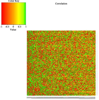
All gene attributes are continuous variables and are scaled before further exploration. The following attributes are binary: “chemo” indicating whether the patient has received a chemotherapy, “hormonal” indicating whether the patient has received hormonal therapy, “amputation” indicating whether forequar-ter amputation has been used as a treatment, “histtype” indicating the histological type. “diam” is a dis-crete variable indicating the diameter of the tumor size, and so is “posnodes” which indicates the number of nodes. But both are considered as continuous variables because they have many levels. Several attributes are categorical variables: “grade” with three levels indicating cancer grade, “angioinv” with three levels in-dicating the extent to which the cancer has invaded blood vessels or lymph vessels, “lymphinfil” with three levels indicating the level of lymphocytic infiltration. These three categorical variables are each trans-formed into three binary variables so that they can feed into more analysis methods. Figure 1 is a heat map to show the correlation:

After attributes investigation, the dataset was further evaluated by different classifiers and prediction methods under 10-fold cross validation scheme [4]. The average squared error, error rate, f1 scores are used as the final metric for performance evaluation.

2.2. Principal Components Analysis (PCA) [5]

(3)

Figure 1. Heat map correlation.

convert the data into a set of directions called Principal Components (PC), ranking by their level of expla-nation of original data’s variance. The transformation is made by multiplication of a loading vector (usually the same dimension as the number of attributes) and the original date.

To maximize the variance explained, the first loading vector can be calculated using:

( )1 =arg maxw=1

{

2

}

=arg maxw=1

{

T T

}

w Xw w X Xw

where X is the original data and w is the loading vector. Then, to calculate the kth_{, first subtract the first (}_k

− 1) PCs from X:

( ) ( ) 1

T 1

k

k n n

n

− =

= −

∑

X X Xw w

Then kth_{loading vector can be calculated:}

( ) _{( )} _{( ) ( )}₁

{

}

_{( )} _{( ) ( )}₁

T T 2

T

1, 0 1, , 0

arg max arg max

k k k k k k

k k k

k ₌ ₋ _⋅ ₌ ₌ ₋ ₌

 

 

= = _ _

 

 

w w w w w w

w X X w

w X w

w w

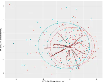
[image:3.595.138.464.75.403.2]

Using PCA, we successfully reduced more than fifteen hundred attributes to 130 attributes while maintaining 90% of the original variance. The reduced dataset is now available for us to perform various machine learning methods.

Figure 2 and Figure 3 show visually how PCA analyzes the data. Both plots are showing how

(4)

[image:4.595.122.477.86.361.2]

Figure 2. PCA of entire data.

[image:4.595.122.477.417.700.2]

(5)

https://doi.org/10.4236/jbise.2018.115008 83 J. Biomedical Science and Engineering 2.3. Regression

Regression models are fit for survival time and recurrence time, and each method is tried separately with clinical-only data, gene-only data and combined data. The results are shown in 6. Model Evaluation. 2.3.1. Linear Regression [6]

Linear regression is a linear approach for modeling the relationship between a scalar dependent vari-able and one or more independent varivari-ables. It is one of the most basic methods in statistical learnings but still has great significance in its application. To achieve the best result possible by linear regression, we used data transformed by PCA and made some adjustments in model selection.

1) Information Criterion and Stepwise Selection

A problem with model selection of linear regression is that as the number of attributes increases, the overall result usually seems to increase as well, but often we require a balance between model simplicity and goodness of fit. In this study, therefore, some information criterions are adopted to find the optimal model for linear regression.

Akaike Information Criterion (AIC) [7] is defined as:

( )

ˆ AIC 2= k−2ln L

where k is the number of estimated parameters and Lˆ is the maximum value of the likelihood function. At the same time, Bayesian Information Criterion (BIC) [8] is defined as:

( )

ˆ

BIC ln= n k−2ln L

where k and Lˆ represent same value in AIC and n is the number of data points in X. BIC works in a sim-ilar way as that of AIC, and they each work better in some cases, so both of them are tried in this study.

For model selection, we used stepwise selection, which is an iterative method that at each iteration, a certain number of attributes are selected and decided to be kept or removed based on the information cri-terion. There are multiple directions for stepwise selection, and in this study we only used forward and backward.

Forward selection starts with no variables in the model and tests the result when each variable is added, finally keeping the variables that improve the statistical significance of the model by the judgment of AIC and BIC. Backward selection, on the other hand, starts with all variables in the model and tests the result when each variable is left out, removing variables that increases AIC or BIC.

2) Shrinkage Method

Shrinkage methods add penalties on parameters in the loss function. It introduces some bias, but could significantly improve the test result. A shrinkage method that can be used as an alternative of model selection is the Lasso method [9]. It solves the following optimization:

1

min p j

j

RSS

β λ ₌ β

 

+

 



∑



where λ is a tuning on the penalty function that balances shrinkage and goodness of fit. With appropriate chosen lambda, the Lasso method can shrink some parameters all the way to zero, thus providing model selection.

2.3.2. Support Vector Machine Regression [10]

Support vector regression is adapted from support vector classifier. It is based on distance between data points, thus is sensitive to high dimensions. Therefore, we used PCA transformed data for this me-thod. After grid search on different kernels, we found that nonlinear kernels work better for both response variables. A nonlinear SVM regression finds that coefficient that minimizes:

( )

(

*

)(

*

)

(

)

(

*

)

(

*

)

1 1 1 1

1 _, _.

2

N N N N

i i j j i j i i i i i

i j i i

L a a a a a G x x ε a a y a a

= = = =

(6)

https://doi.org/10.4236/jbise.2018.115008 84 J. Biomedical Science and Engineering where G is the Gram matrix of the original data. The conditions are:

(

*

)

1 0

N

n n

n= a a

− =

∑

: 0 _n

n a C

∀ ≤ ≤

*

: 0 _n .

n a C

∀ ≤ ≤

Parameters ε and C (cost) are tuned before finding the best result. 2.3.3. Bagging and Random Forest Regression [11]

Bagging and random forest are bootstrap aggregating methods applied to decision trees (details in 4.4. Decision Tree) to mainly solve the problem of over-fitting. In both methods, multiple samples of cer-tain variables are taken into consideration to be split in nodes, and the result is the average of these trees. The difference between bagging and random forest is that bagging consider all variables in each bootstrap, while random forest picks a portion of variables. Both methods handle high-dimension comparatively well, thus we feed in the full data.

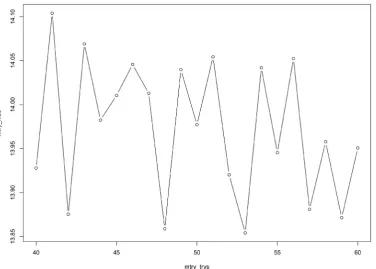
There are multiple parameters that require tuning to achieve optimal random forest models. Using 10-fold cross validation, we tuned the number of variables selected at each iteration (Figure 4) and the maximum of nodes generated (Figure 5).

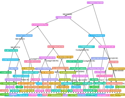
Figure 6 and Figure 7 can roughly represent the models (it is impractical to visualize all fifteen hun-dred attributes).

2.4. Classification

[image:6.595.114.491.431.700.2]

Classification models are fit for mortality and each method is tried with clinical-only data, gene-only data and combined data. Whether data transformed by PCA or full data is used depended on the specific method used. The results are in 6.1. Model Selection.

(7)

[image:7.595.104.497.71.355.2]

Figure 5. Tuning random forest: maximum number of nodes.

[image:7.595.92.509.383.704.2]

(8)

[image:8.595.82.516.71.412.2]

Figure 7. Random forest: Survival time.

2.4.1. Bayesian Logistic Regression [12]

Bayesian logistic regression works in a similar way of traditional logistic regression. However, it starts with an assumption of distribution of p

(

β β0, 1

)

, usually normal distribution, then maximize the

likelih-ood function:

(

)

1

1 1

i i

n _y

y

i i

i p p

− =

−

∏

where yi is the response variable (mortality in this case) and the probability pi is defined as:

( )

exp 1 exp

t i

i _t

i

p β

β =

+ x

x

where β denotes the contribution an independent variable makes in determining the classification of the dependent variable. Data transformed by PCA is used for this method.

2.4.2. Linear Discriminant Analysis (LDA) [13]

LDA is an unsupervised learning method that can separate data into two or more classes. It is closely related to analysis of variance (ANOVA) and is similar to PCA in this aspect. However, it focuses more on the difference between classes.

LDA assumes that the conditional probability density functions p

(

x y =0

)

_and p

(

x y =1

)

_are both normally distributed with mean and covariance parameters

(

µ0,Σ0

)

and

(

µ1,Σ1

)

. We predict that

(9)

(

)

1

(

)

(

)

1

(

)

0 0 1

T T

0 0 ln 1 1 ln 1

x₋µ _Σ− x₋µ ₊ _Σ ₋ x₋µ _Σ− x₋µ ₋ _Σ _>T

       

where T, here for two classes without specified weights, is 0.5. Full data is used for this method. 2.4.3. K-Nearest Neighbor (KNN) [14]

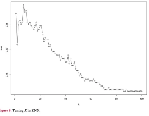
KNN is another popular method that uses distance between points to achieve classification, thus making it sensible to high dimensions, so data transformed by PCA is used here. The class of a certain data point is determined by a majority vote of k nearest neighbors” classes. Parameter k is tuned in Figure 8

(the mse here is 10-fold cross validation result). 2.4.4. Decision Tree [15]

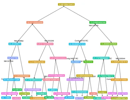
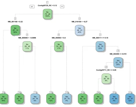
Decision tree uses tree-like graph to represent each decision that leads to the last classification or re-gression result. It uses an iterative logarithm that at each iteration, the tree is split at where the smallest RSS would be produced. The parameter that limited the minimum amounts of leaves produced is tuned to be optimal first. The tree based methods generally handle high-dimensions better, thus we feed the full data. Figure 9 can roughly represent the tree built.

2.4.5. Random Forest Classification

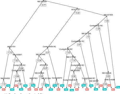
[image:9.595.62.541.363.735.2]

A random forest classifier works in a very similar way as a random forest regression model described in 3.3. Bagging and Random Forest Regression. Same parameters that are tuned in random forest regres-sion are tuned here as well. Because it is a tree based method, we feed in the full data and will also use this method for top gene selection. Figure 10 can roughly represent the model.

(10)

[image:10.595.66.536.72.441.2]

Figure 9. Decision tree: Survivability.

2.4.6. Adaptive Boosting [16]

Adaptive boosting is another ensemble method that evaluates the classification error during the process of readjusting weights. In this study, the adaptive boosting is based on decision trees, so we feed full data into it. We tuned the number of iteration.

2.4.7. Support Vector Machine Classification (SVM)

SVM classifier puts data points into p-dimensional space where p is the number of attributes. Then it creates two hyperplanes to separate the space into two regions, thus achieving classification. The argument of SVM is:

( )

, ₁

min ,

2

N _i

w b _i

w

C ξ

=

+

∑

( )

(

T

( )

)

( ) subjgate to :_yi _w _∅ _xi ₊_b _{≥ −}1 _ξ i

( )i _0,

_{

_{1, ,}

_}

i N

ξ ≥ ∀ ∈ 

where _ξ( )i _{is the slack variable and}_C_{is the penalty of error term}_i.e._cost. _∅_{is the function that maps}

(11)

[image:11.595.74.535.76.438.2]

Figure 10. Random forest: Survivability.

2.5. Gene Selection

Random forest method, or rather decision tree, provides an insight into feature selection. Trees are built from root to leaves, and the closer a variable is to the root, generally, the more important it is. For all three response variables, optimal parameters for a random forest model are already found. Three separate models are fit using the entire data, and by setting the “importance” parameter to be true, top attributes can be found for each response variable.

3. RESUULTS AND CONCLUSION

3.1. Model Evaluation

The regression models are evaluated through squared error and classification methods through error rate and f1 score. All the results below are 10-fold cross validation result, each representing the optimal result of that method.

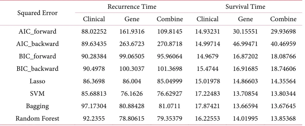
3.2. Regression

Table 1 shows the regression performance of each method. For recurrence time models, support

(12)

[image:12.595.57.543.95.296.2]

Table 1. Regression result.

Squared Error Recurrence Time Survival Time

Clinical Gene Combine Clinical Gene Combine

AIC_forward 88.02252 161.9316 109.8145 14.93231 30.15551 29.93698 AIC_backward 89.63435 263.6723 270.8718 14.99714 46.99471 40.46959 BIC_forward 90.28384 99.06505 95.96064 14.9679 16.87202 18.08766 BIC_backward 90.4978 100.3037 101.3698 15.4744 16.91685 18.74606 Lasso 86.3698 86.004 85.04999 15.01978 14.86603 14.35564 SVM 85.68813 76.1626 76.62927 17.22483 13.70854 13.80344 Bagging 97.17304 80.88428 81.0711 17.87421 13.66594 13.67645 Random Forest 92.2355 78.80615 79.35379 16.22553 14.01995 13.85368

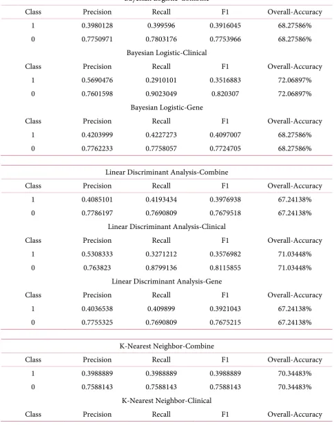
3.3. Classification

Table 2 shows the classification performance of each model. For classification, the best model comes

by K-Nearest Neighbor on clinical data only, with an overall accuracy of 88.97% and f1 score of 0.7518. A couple of ROC curves are drawn for a couple of methods for visualization (Figures 11-14). ROC curves show how a classification method works. The larger the area under the curve (AUC), the better is the clas-sification i.e. the closer the curve is to the top left corner, the better the model is. Plots below show the comparisons between the use of only gene data, only clinical data, and combined data. For classification methods such as random forest (Figure 13), for example, using only gene data or combined data proved to be better than using only clinical data.

3.4. Application

Table 3 shows a case example of our treatment optimization method. Given a patient with specific

clinical attributes, represented by “posnodes”, and unique gene information, we start by assuming that the patient does not take any treatment, so the inputs for “chemo,” “hormonal,” and “amputation” are all zero. Then, we test if chemotherapy would work by changing “chemo” to one while keeping other parameters the same. Then using our model, we find the survival time more than doubles. This indicates the effect of chemotherapy on this specific patient without actual clinical attempts. To further investigate, we also change amputation to one, but the survival time drops. This result suggests that combing chemotherapy and amputation may not work the best for this specific patient.

Suppose there are n treatments available, then, by comparing the results of 2n_{possible combinations,}

an individualized optimal treatment plan can be determined for a specific patient at the cost of mere computation power.

3.5. Corroboration on Gene Importance

Table 4 shows the top genes selected using random forest method and its importance parameter.

Several genes are found to be biological-studies supported. The most significant ones are: 1) NM_014585

Homo sapiens solute carrier family 40 member 1 (SLC40A1), mRNA.

(13)

[image:13.595.55.541.107.724.2]

Table 2. Classification result.

Bayesian Logistic-Combine

Class Precision Recall F1 Overall-Accuracy

1 0.3980128 0.399596 0.3916045 68.27586%

0 0.7750971 0.7803176 0.7753966 68.27586%

Bayesian Logistic-Clinical

1 0.5690476 0.2910101 0.3516883 72.06897%

0 0.7601598 0.9023049 0.820307 72.06897%

Bayesian Logistic-Gene

1 0.4203999 0.4227273 0.4097007 68.27586%

0 0.7762233 0.7758057 0.7724705 68.27586%

Linear Discriminant Analysis-Combine

1 0.4085101 0.4193434 0.3976938 67.24138%

0 0.7786197 0.7690809 0.7679518 67.24138%

Linear Discriminant Analysis-Clinical

1 0.5308333 0.3271212 0.3576982 71.03448%

0 0.763823 0.8799136 0.8115855 71.03448%

Linear Discriminant Analysis-Gene

1 0.4036538 0.409899 0.3921043 67.24138%

0 0.7755325 0.7690809 0.7675215 67.24138%

K-Nearest Neighbor-Combine

1 0.3988889 0.3988889 0.3988889 70.34483%

0 0.7588143 0.7588143 0.7588143 70.34483%

K-Nearest Neighbor-Clinical

(14)

https://doi.org/10.4236/jbise.2018.115008 92 J. Biomedical Science and Engineering Continued

1 0.9107143 0.6568687 0.7518273 88.96552%

0 0.8804512 0.9823043 0.9268241 88.96552%

K-Nearest Neighbor-Gene

1 0.5291667 0.2767172 0.3487332 72.75862%

0 0.7602304 0.901597 0.8224293 72.75862%

Decision Tree-Combine

1 0.511241 0.4384343 0.4433902 70.34483%

0 0.7805227 0.8257206 0.7963284 70.34483%

Decision Tree-Clinical

1 0.5509524 0.3108586 0.3670707 70.68966%

0 0.7591357 0.8680392 0.8059787 70.68966%

Decision Tree-Gene

1 0.5029076 0.4293434 0.4319616 70.00000%

0 0.7779074 0.8257206 0.7945314 70.00000%

Random Forest-Combine

1 0.5213095 0.2500505 0.3244089 73.931%

0 0.7553637 0.9086234 0.8220094 73.931%

Random Forest-Clinical

1 0.5993651 0.3543434 0.4028256 72.75862%

0 0.7727882 0.8843049 0.818625 72.75862%

Random Forest-Gene

1 0.4683333 0.2250505 0.2883832 71.37931%

(15)

https://doi.org/10.4236/jbise.2018.115008 93 J. Biomedical Science and Engineering Adaptive Boosting-Combine

1 0.4952381 0.2865657 0.3440309 70.0000%

0 0.7578552 0.8571818 0.7992672 70.0000%

Adaptive Boosting-Clinical

1 0.4566667 0.4363636 0.4016618 67.24138%

0 0.7787268 0.7857737 0.7695106 67.24138%

Adaptive Boosting-Gene

1 0.5361905 0.3635859 0.3995099 72.06897%

0 0.7713405 0.8691818 0.8118039 72.06897%

SVM-Combine

1 0.6203704 0.2087374 0.3300298 74.48276%

0 0.7539762 0.9561378 0.8405229 74.48276%

SVM-Clinical

1 0.6733333 0.2934343 0.381746 75.86207%

0 0.770486 0.9553455 0.8485846 75.86207%

SVM-Gene

1 0.687037 0.2361616 0.3651675 68.7037%

[image:15.595.52.546.637.725.2]

0 0.7591547 0.9461378 0.8401366 68.7037%

Table 3. Case example of treatment optimization.

ID Survival Time Chemo Hormonal Amputation Posnodes Gene Info

18 6.2587 0 0 0 2 ∙∙∙

18 14.8172 1 0 0 2 ∙∙∙

(16)

[image:16.595.104.493.71.370.2]

[image:16.595.101.513.319.699.2]

Figure 11. ROC curve: Bayesian logistic.

(17)

[image:17.595.103.492.92.532.2]

[image:17.595.106.496.257.690.2]

Figure 13. ROC curve: Random forest.

(18)

[image:18.595.63.538.95.315.2]

Table 4. Significant genes.

Recurrence Survival Time Mortality

1 NM_014585 Contig48156_RC NM_003890

2 NM_001609 NM_014585 NM_003891

3 NM_020974 NM_001635 NM_006787

4 NM_016569 AB040926 AF131851

5 NM_001565 AL117638 U47671

6 NM_018410 NM_020974 AF103458

7 NM_018265 NM_001333 Contig45703_RC

8 NM_004244 NM_014112 Contig32798_RC

9 AB040900 NM_002427 Contig50822_RC

10 NM_005940 Contig34303_RC NM_002426

*Note that these gene names are accession numbers.

NRIP3) and metal ion binding (CYP4Z1, CYP4Z2P, SLC40A1, LTF, LIMCH1). And “PIK3CA, encoding the PI3K catalytic subunit, is the oncogene exhibiting a high frequency of gain-of-function mutations leading to PI3K/AKT pathway activation in breast cancer” [17].

2) NM_001609

Homo sapiens acyl-CoA dehydrogenase short/branched chain (ACADSB), transcript variant 1, mRNA.

A research studying breast cancer in Chinese women concluded that “Of the studied SNPs, only rs12570116 in ACADSB, rs10902845 in C10orf88, rs4760658 in VDR, and rs6091822, rs8124792 and rs6097809 in CYP24A1 had a nominal association” [18].

3) NM_020974

Homo sapiens signal peptide, CUB domain and EGF like domain containing 2 (SCUBE2), transcript variant 1, mRNA.

SCUBE2 was found to be expressed in invasive breast carcinomas: “In this report, we show by anti-SCUBE2 immunostaining that SCUBE2 is mainly expressed in vascular endothelial and mammary ductal epithelial cells in normal breast tissue. In addition, we observed positive staining for SCUBE2 in 55% (86 of 156) of primary breast tumors.” The entire report above shows the role of SCUBE2 in breast cancer and the specific mechanisms of how SCUBE2 influence the outcome of the breast cancer [19].

4) NM_016569

Homo sapiens T-box 3 (TBX3), transcript variant 2, mRNA.

A medical research states that, “reduction of FGFR or TbX3 gene expression was able to abrogate tumorsphere formation, whereas ectopic TbX3 expression increased tumor seeding potential by 100-fold” [20].

5) NM_001565

Homo sapiens C-X-C motif chemokine ligand 10 (CXCL10), mRNA.

CXCL10 is found to lead to breast cancer: “activation of Ras plays a critical role in modulating the expression of both CXCL10 and CXCR3-B, which may have important consequences in the development of breast tumors through cancer cell proliferation” [21].

6) NM_003890

(19)

https://doi.org/10.4236/jbise.2018.115008 97 J. Biomedical Science and Engineering FCGBP is a gene family that has been found to have an independent influence on the progression of carcinoma: “Immunochemistry and clinic pathological results showed that the expression of NT5E and FCGBP in gallbladder adenocarcinoma is an independent marker for evaluation of the disease progres-sion, clinical biological behaviors and prognosis” [22].

7) NM_003891

Homo sapiens protein Z, vitamin K dependent plasma glycoprotein (PROZ), transcript variant 2, mRNA.

PROZ is found to be in support of the spread of tumor cells: “In line with our functional findings, PROZ expression has been observed in several human cancers, suggesting that the PROZ/ZPI complex might support the invasion and metastasis of tumor cells” [23].

8). NM_002426

Homo sapiens matrix metallopeptidase 12 (MMP12), mRNA.

MMP family members usually represent the host response to the tumor of breast cancer: “These re-sults indicate that there is very tight and complex regulation in the expression of MMP family members in breast cancer that generally represents a host response to the tumor and emphasize the need to further evaluate differential functions for MMP family members in breast tumor progression” [24].

4. DISCUSSION

This study stands out in its comprehensive understanding of cancer genomics. Not only could the result help precisely predict breast cancer survivability, but it can also predict recurrence and survival time. Aside from modeling, the study identifies certain genes that could further help with clinical progno-sis. The methodology used in this study can be applied to more disease learning, especially those with high dimensional data such as genomics, to not only achieve better clinical prediction but identification of sig-nificant attributes of the patient that worth biological researches.

This research, most importantly, demonstrates an application of the core idea of big data to the med-ical field. For more diseases, even those beyond cancer scope, such methodology of modeling and explora-tion can be applied. For example, given a lung cancer data in a format similar to what we used in this study, we could develop such treatment optimization and gene selection system using the methods dis-cussed. Choices of clinical attributes, such as gender of the patient and some basic physical measurements, may be specified according to lung cancer; along with gene attributes, a gigantic scale of parameters can be provided for a single patient. The training dataset should also include several possible treatments for lung cancer as attributes, and several clinical outcomes as response variables. Once the best model is developed using methods discussed in this research, it can be used to determine the best combination of treatments to achieve optimal clinical outcomes (6.3. Application).

In the recent years, similar efforts were made to develop customized cancer treatments. The idea, basically, is to investigate the patient’s gene and how it is correlated with the cancer. Then, they develop medicines that targeted these genes specific for this certain patient. Nevertheless, there are certain limita-tions to this method. The idea requires meticulous lab work and investigation, which makes it time con-suming and expensive. Also, though we have learnt some biomarkers and cancer-related pathways, cancer genomics are not fully understood yet, let alone disease genomics for many other diseases. At current stage of cancer research, this method inevitably introduces error.

(20)

https://doi.org/10.4236/jbise.2018.115008 98 J. Biomedical Science and Engineering optimal combination of treatment seconds upon diagnosis, helping them make better decisions and avoid unnecessary cost.

There are three main ways through which we may increase the applicability of the research and finally achieve the goal described above. First, more advanced machine learning or deep learning method are al-ways possible to improve the model result. Second, the bigger the data is and the longer period over which the data is collected, the more reliable the model will be since less bias will be generated. Finally, several attributes (gene or clinical) and treatments may have correlations among themselves. If they can be un-derstood thoroughly, the attributes representing them can be pre-processed to avoid collinearity. For in-stance, if a gene is biologically proved to be closely related to certain disease, the weight of that gene input can be increased; if certain medical treatment targets certain gene, some transformation of the two attri-buted could be processed before modeling. Through this vertical improvement of the result of certain ap-plication (such as the one discussed in this study), and horizontal expansion that includes more and more medical areas (generalization of the idea proposed by this study), future hospitals can provide a compre-hensive and systematic procedure to present the patient with crystal clear choices and possibilities.

REFERENCES

1. Trop, I., Dugas, A., David, J., El Khoury, M., Boileau, J.F., Larouche, N. and Lalonde, L. (2011) Breast Abscesses: Evidence-Based Algorithms for Diagnosis, Management, and Follow-Up. Radiographics, 31, 1683-1699.

https://doi.org/10.1148/rg.316115521

2. Edgar, R., Domrachev, M. and Lash, A.E. (2002) Gene Expression Omnibus: NCBI Gene Expression and Hybri-dization Array Data Repository. Nucleic Acids Research, 30, 207-210. https://doi.org/10.1093/nar/30.1.207

3. Ramanan, D. and Angelov, B. (2016) NKI Breast Cancer Data.

https://data.world/deviramanan2016/nki-breast-cancer-data

4. Kohavi, R. (1995) A Study of cross-validation and Bootstrap for Accuracy Estimation and Model Selection. In Ijcai, 14, 1137-1145.

5. Jolliffe, I.T. (1986) Principal Component Analysis and Factor Analysis. In: Principal Component Analysis, Springer, New York, 115-128. https://doi.org/10.1007/978-1-4757-1904-8_7

6. Neter, J., Kutner, M.H., Nachtsheim, C.J. and Wasserman, W. (1996) Applied Linear Statistical Models. Vol. 4, Irwin, Chicago, 318.

7. Sakamoto, Y., Ishiguro, M. and Kitagawa, G. (1986) Akaike Information Criterion Statistics.

8. Akaike, H. (1976) Canonical Correlation Analysis of Time Series and the Use of an Information Criterion. Ma-thematics in Science and Engineering, 126, 27-96. https://doi.org/10.1016/S0076-5392(08)60869-3

9. Tibshirani, R. (1996) Regression Shrinkage and Selection via the Lasso. Journal of the Royal Statistical Society,

Series B (Methodological), 73, 267-288.

10. Cortes, C. and Vapnik, V. (1995) Support Vector Machine. Machine Learning, 20, 273-297.

https://doi.org/10.1007/BF00994018

11. Breiman, L. (2001) Random Forests. Machine Learning, 45, 5-32. https://doi.org/10.1023/A:1010933404324

12. Hosmer Jr., D.W., Lemeshow, S. and Sturdivant, R.X. (2013) Applied Logistic Regression. Vol. 398, John Wiley & Sons, Hoboken.

13. McLachlan, G.J. (2004) Discriminant Analysis and Statistical Pattern Recognition. Wiley Interscience, Hoboken. 14. Cover, T. and Hart, P. (1967) Nearest Neighbor Pattern Classification. IEEE Transactions on Information

Theory, 13, 21-27. https://doi.org/10.1109/TIT.1967.1053964

15. Quinlan, J.R. (1987) Simplifying Decision Trees. International Journal of Man-Machine Studies, 27, 221-234.

(21)

16. Freund, Y. and Schapire, R.E. (1996) Experiments with a New Boosting Algorithm. Proceedings of the 13th In-ternational Conference on InIn-ternational Conference on Machine Learning, Bari, 3-6 July 1996, Vol. 96, 148-156. 17. Cizkova, M., Cizeron-Clairac, G., Vacher, S., Susini, A., Andrieu, C., Lidereau, R. and Bièche, I. (2010) Gene

Expression Profiling Reveals New Aspects of PIK3CA Mutation in ERalpha-Positive Breast Cancer: Major Im-plication of the Wnt Signaling Pathway. PLoS ONE, 5, e15647. https://doi.org/10.1371/journal.pone.0015647

18. Dorjgochoo, T., Delahanty, R., Lu, W., Long, J.R., Cai, Q., Zheng, Y., Shu, X.O., et al. (2011) Common Genetic Variants in the Vitamin D Pathway Including Genome-Wide Associated Variants Are Not Associated with Breast Cancer Risk among Chinese Women. Cancer Epidemiology, Biomarkers & Prevention, 20, 2313-2316. https://doi.org/10.1158/1055-9965.EPI-11-0704

19. Cheng, C.J., Lin, Y.C., Tsai, M.T., Chen, C.S., Hsieh, M.C., Chen, C.L. and Yang, R.B. (2009) SCUBE2 Sup-presses Breast Tumor Cell Proliferation and Confers a Favorable Prognosis in Invasive Breast Cancer. Cancer Research, 69, 3634-3641. https://doi.org/10.1158/0008-5472.CAN-08-3615

20. Fillmore, C.M., Gupta, P.B., Rudnick, J.A., Caballero, S., Keller, P.J., Lander, E.S. and Kuperwasser, C. (2010) Estrogen Expands Breast Cancer Stem-Like Cells through Paracrine FGF/Tbx3 Signaling. Proceedings of the National Academy of Sciences, 107, 21737-21742. https://doi.org/10.1073/pnas.1007863107

21. Datta, D., Flaxenburg, J.A., Laxmanan, S., Geehan, C., Grimm, M., Waaga-Gasser, A.M., Pal, S., et al. (2006) Ras-Induced Modulation of CXCL10 and Its Receptor Splice Variant CXCR3-B in MDA-MB-435 and MCF-7 Cells: Relevance for the Development of Human Breast Cancer. Cancer Research, 66, 9509-9518.

https://doi.org/10.1158/0008-5472.CAN-05-4345

22. Xiong, L., Wen, Y., Miao, X. and Yang, Z. (2014) NT5E and FcGBP as Key Regulators of TGF-1-Induced Epi-thelial-Mesenchymal Transition (EMT) Are Associated with Tumor Progression and Survival of Patients with Gallbladder Cancer. Cell and Tissue Research, 355, 365-374. https://doi.org/10.1007/s00441-013-1752-1

23. Neumann, O., Kesselmeier, M., Geffers, R., Pellegrino, R., Radlwimmer, B., Hoffmann, K., Longerich, T., et al. (2012) Methylome Analysis and Integrative Profiling of Human HCCs Identify Novel Protumorigenic Factors.

Hepatology, 56, 1817-1827. https://doi.org/10.1002/hep.25870