15
Detecting Network Intrusion through a Deep Learning
Approach
Abhilasha Jayaswal
Student
Indore, MP
Romit Nahar
Student
Indore, MP
ABSTRACT
Intrusion Detection: collection of techniques that are used to identify attacks on the computers and network infrastructures. Anomaly detection, which is a key element of intrusion detection. In Anomaly Detection, perturbations of normal behavior suggest the presence of intentionally or unintentionally induced attacks, faults, defects, etc. This paper focuses on an approach based on deep learning to develop an effective and flexible network intrusion detection system implemented using self-taught learning on NSL-KDD data set.
General Terms
Intrusion Detection, Network, anomalous traffic.
Keywords
Deep learning, Network Security, NIDS, sparse auto encoder.
1.
INTRODUCTION
The intrusion detection problem is becoming an exigent task due to the escalation of heterogeneous computer networks since the increase in connectivity of computer systems gives more access to no-members and makes it easier for intruders to avoid identification. Intrusion Detection Systems (IDSs) are based on the assumption that an unauthorized user's conduct will always be different from that of an authorized user and most of the unauthorized/illegal actions are also identifiable [1].
1) Signature (Misuse) based NIDS (SNIDS), and 2) Anomaly Detection based NIDS (ADNIDS) are the two classes in which NIDSs are categorized based on the methods of Intrusion Detection. The Signature-based Intrusion Detection Systems follow a lot similar procedure as a virus scanner. They search for a known member's id or signature for each particular intrusion incident. And, while signature-based IDS is very efficient at sniffing out known attack, it does, like anti-virus software, depend on receiving regular signature updates, to keep in touch with variations in hacker technique. Expressing in different way, SIDSs is limited to the system’s database of stored signatures.
An anomaly-based IDS works by first building a statistical model of usage patterns describing the normal behavior of the monitored resource. After this initial training phase, the system uses a similarity metric to compare new input requests
with the model, and generates alerts for those deviating significantly, considering them anomalous. Basically, in this, intrusions are detected as they produce a dissimilar, i.e., abnormal, behavior then what was noticed while designing the model. Its ability to detect previously unknown (or variants of known) attacks when they appear is the biggest advantage of an Anomaly-based System [2].
Two challenges that arise while developing an effective and adaptable NIDS for upcoming attacks, in future, that are not known: Firstly, selection of all features from the Network Traffic dataset for anomaly detection is difficult. The features selected for one class of attack may not work well for other categories of attacks due to continuously changing and evolving attack scenarios. Second, unavailability of labeled traffic dataset from real networks for developing an NIDS [3].
Numerous machine learning techniques such as Support Vector Machines (SVM), Random Forests (RF), Artificial Neural Networks (ANN), Naïve- Bayesian (NB), etc. NIDS are classifiers that differentiate unauthorized or anomalous traffic from authorized or normal traffic. Many NIDSs perform a feature selection task to extract a subset of relevant features from the traffic dataset to enhance classification results. Feature selection helps in the elimination of the possibility of incorrect training through the removal of redundant features and noises.
16
Figure 1: Two-staged process of self-taught learning: a) Unsupervised Feature Learning (UFL) on unlabeled data. b) Classification on labeled data.
2.
OVERVIEW
OF
SELF
TAUGHT
LEARNING AND NSL-KDD DATASET
2.1 Self Taught Learning
Self -taught learning is a machine learning framework for using unlabeled data in supervised classification tasks. Self-taught Learning (STL) is a deep learning approach that consists of two stages for the classification. First, a good feature representation is learnt from a large collection of unlabeled data, 𝑥𝑢, termed as Unsupervised Feature Learning
(UFL). In the second stage, this learnt representation is applied to labeled data, 𝑥𝑙, and used for the classification task.
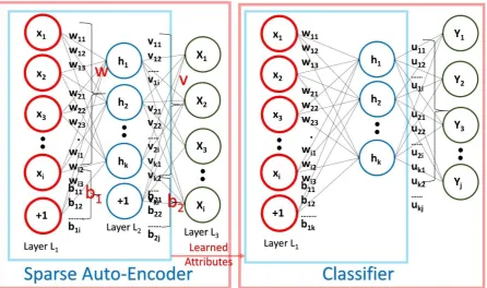
There must be relevance between the unlabeled and labeled data, although they may come from distinct distributions. Figure 1 shows the architecture diagram of STL. Sparse Auto-Encoder, K-Means Clustering, Restricted Boltzmann Machine (RBM), and Gaussian Mixtures [4], are some approaches used for UFL. The Sparse Auto-Encoder based feature learning is used for this work due to its easy implementation and good performance.
The input and output layers contain 𝑁 nodes and the hidden layer contains 𝐾 nodes. The target values in the output layer set to the input values, i.e.,𝑥 𝑖 = 𝑥𝑖 as shown in Figure 1(a). The sparse auto-encoder network finds the optimal values for weight matrices,𝑊 ∈ 𝑅𝐾×𝑁 and 𝑉 ∈ 𝑅𝑁×𝐾, and bias vectors, 𝑏1∈ 𝑅𝐾 and 𝑏1∈ 𝑅𝑁, using back-propagation algorithm
while trying to learn the approximation of the identity function, i.e., output 𝑥 similar to 𝑥. Sigmoid function,
𝑔(𝑧) = 1
1−𝑒−𝑧, is used for the activation,ℎ𝑊,𝑏 of the nodes in the hidden and output layers:
ℎ𝑊,𝑏 𝑥 = 𝑔 𝑊𝑥+ 𝑏 … (1)
𝐽 = 1
2𝑚 | 𝑥𝑖− 𝑥 |𝑖 2 𝑚
𝑖=1 +
𝜆
2 𝑊 2
𝑘,𝑛 + 𝑉 2 𝑛,𝑘 + 𝑏12
𝑘 + 𝑏2 2
𝑛 + 𝛽 𝐾𝐿 𝐾
𝑗 =1 (𝜌||𝜌 )𝑗 …(2)
The cost function to be minimized in sparse auto-encoder using back-propagation is represented by equation 2. The first term is the average of sum-of-square errors term for the all 𝑚
input data. The second term is a weight decay term, with 𝜆 as eight decay parameters, to avoid the over-fitting in training. The final term in the equation is Sparsity Penalty term that puts a constraint into the hidden layer to maintain a low average activation values, and expressed as Kullback-Leibler (KL) divergence shown in equation 3:
𝐾𝐿(𝜌| 𝜌 𝑗 = 𝜌 log 𝜌 𝜌𝑗
+ 1 − 𝜌 log1 − 𝜌 1 − 𝜌𝑗
where, 𝜌 is a sparsity constraint parameter ranges from 0 to 1 and 𝛽 controls the sparsity penalty term.
The 𝐾𝐿(𝜌| 𝜌 𝑗 attains a minimum value when 𝜌 = 𝜌 𝑗 , where 𝜌 𝑗 denotes the average activation value of hidden unit 𝑗 over
the all training inputs, 𝑥. Once, the optimal values for 𝑊 and
𝑏1 are learnt by applying the sparse auto-encoder on unlabeled data, 𝑥𝑢, thereafter, the feature representation is
17
2.2 NSL-KDD Dataset
[image:3.595.53.283.274.399.2]As mentioned previously, the NSL-KDD dataset is used in this work. NSL KDD here refers to Network Socket Layer KDD. The dataset is an improvised and reduced version of the KDD Cup 99 dataset [5]. The KDD Cup dataset was prepared using the network traffic recorded by DARPA's 1998 IDS evaluation program [6]. The network traffic incorporates both normal or authorized and different kinds of attack traffic, like DoS, Probing. The network traffic for training was collected for seven weeks followed by the two weeks collection of traffic for testing purpose in the form of raw TCP dump format. The test data contains many attacks that were not injected during the training data collection phase to make the intrusion detection task realistic. Researchers believe that known attacks can be used to derive most of the novel attacks.
Table 1: Traffic records distribution in the training and test data for normal and attack traffic
Track
Training
Test
Normal
67343
9711
Attack
DoS
45927
7458
U2R
52
67
R2L
995
2887
Probe
11656
2421
Thenceforth, the training and test data were processed into the datasets of five million and two million TCP/IP connection records, respectively. For evaluation of NIDS, the KDD Cup dataset has been widely used as a benchmark dataset for many years. One of the major drawback with the dataset is that it contains an enormous amount of redundant records both in the training and test data. According to observations almost 78% of training and 75% test data records are redundant. This redundancy makes the learning algorithms biased towards the frequent attack records and leads to poor classification results for the infrequent, but harmful records. The training and test data were classified with the minimum accuracy of 98% and 86% respectively using a very simple machine learning algorithm. It made the comparison task difficult for various IDSs based on different learning algorithms. NSL-KDD was proposed to overcome the limitation of KDD Cup dataset. The dataset is imitative of the KDD Cup dataset [4].
NSL-KDD improvised the previous dataset in two ways. Firstly, it exterminated all the redundant records present in the training and test data. Secondly, it apportioned all the records present in the KDD Cup dataset into discrete levels of difficulty based on the number of learning algorithms that can correctly classify the records. After that, it selected the records by random sampling of the distinct records from each difficulty level in a fraction that is inversely proportional to their fraction in the distinct records. These multi-steps processing of KDD Cup dataset made the number of records in NSL-KDD dataset reasonable for the training of any learning algorithm and realistic as well. In NSL-KDD dataset
each record consists of 41 features and is labeled as either normal or a particular kind of attack. These features include basic features derived directly from a TCP/IP connection, traffic features accumulated in a window interval, either time, e.g. two seconds or number of connections, and content features extracted from the application layer data of connections. Out of 41 features, three are nominal, four are binary, and remaining 34 features are continuous.
3.
RESULTS
3.1
Implementing NIDS
As mentioned previously, the dataset contains different kinds of attributes with different values. The dataset is preprocessed before applying self-taught learning on it. Nominal attributes are converted into discrete attributes using 1-to-n encoding. In addition, there is one attribute in the dataset whose value is always 0 for all the records in the training and test data. This attribute is eliminated from the dataset. The total number of attributes become 121 after performing the above-mentioned steps. The values in the output layer during the feature learning phase, is computed by the sigmoid function which gives values from 0 to 1. Since, the output layer values are identical to the input layer values in this phase, causes to normalize the values in the input layer from 0 to 1.
Then the max min operations are performed on the new list of attributes, to obtain this. The NSL-KDD training data without labels is used with the new attributes for the feature learning using sparse auto-encoder for the first stage of self-taught learning. In the second stage, the new learned features representation is applied on the training data itself for the classification using soft-max regression. In this implementation, both the unlabeled and labeled data for feature learning and classifier training come from the same source, i.e., NSL-KDD training data.
3.2
Metrics for Accuracy
To evaluate the performance of self-taught learning the metrics mentioned below is used:
• Accuracy: Measure of accuracy is the percentage of records that are classified correctly over total number of records.
• Recall(R): Recall is measure as percentage ratio of number of records that are true positives divide by number of records that are classified as True Positives(TP) and False Negatives(FN).
R= 𝑇.𝑃
𝑇.𝑃+𝐹.𝑁∗ 100%
• Precision(P): Precision is measured as the percentage ratio of number of records that are True Positives divided by the number of True Positive and False Positives(FP).
P= 𝑇.𝑃
𝑇.𝑃+𝐹.𝑃∗ 100%
• F Measure(F): F Measure is equivalent to the harmonic mean of recall and precision. F represents a balance between R and P.
F= 2.𝑃.𝑅
𝑃+𝑅
18
3.3
Evaluation of the Performance of NIDS
[image:4.595.314.542.73.233.2]NIDS has been implemented for two different types of classifications: a) Normal and anomaly (2-class) and b) Normal and four different attack categories (5-class). The values of precision, recall and f measure are evaluated for the attacks in the case of 2-class and 5-class classification.
Figure 2: Values of precision, recall and F-measure obtained using STL and SMR for 2-Class when applied on
[image:4.595.312.543.79.446.2]training data
Figure 3: Accuracy of classification using STL and SMR for 2-class and 5-class when applied on test data
3.3.1
Training Data Based Evaluation
In order to evaluate the classification accuracy of self-taught learning for 2-class and 5-class 10-fold cross-validation is applied on the training data. Further, its performance is compared with soft-max regression (SMR) when directly applied on dataset without feature learning. For 2-class classification STL performs better than SMR and in case of 5-class 5-classification its performance is similar. From figure 2 it is evident that STL achieved classification accuracy rate more than 98% for all types of classification [7].
The values of precision, recall, and f-measure values for only 2-class classification is measured. A few kinds of records were missing while performing 10-fold cross-validation during the training or test phase for 5-class classification. Therefore, evaluation of these metrics for 2-class only is done. It was observed that STL achieved better values for all these metrics as compared to SMR.
[image:4.595.52.282.138.498.2]According to the evaluation using training data, it has been established that performance of STL is comparable to the best results obtained in various previous work.
Figure 4: Precision, Recall, and F-Measure values using self-taught learning (STL) and soft-max regression (SMR)
for 2-class when applied on test data
Figure 5: Precision, Recall, and F-Measure values using self-taught learning (STL) and soft-max regression (SMR)
for 5-class when applied on test data
3.3.2
Training and Test Data Based Evaluation
STL’s performance is evaluated for 2-class and 5-class classifications using the test data. As visible in Figure 3 that STL performs very well as compared to SMR. For the 2-class classification, STL achieved 88.39% accuracy rate, whereas SM achieved 78.06%. STL’s accuracy for 2-class classification outshines many of the previous work results.
The values of precision, recall, and f-measure as per Figure 4 and Figure 5 for 2-class and 5-class. STL achieved lower precision as compared to SM, for the 2-class. The precision values for STL and SM are 85.44% and 96.56%, respectively. However, STL achieved better recall values as compared to SM, that are 95.95% and 63.73%, respectively. Due to a good recall value, STL out-performed SM for the f-measure value. STL achieved 90.4% f-measure value whereas SM achieved only 76.8%. Similar observations were made for the 5-class as in the case of 2-class shown in Figure 7. The f-measure values for STL and SM are 75.76% and 72.14%, respectively [7].
4.
CONCLUSION AND FUTURE WORK
Proposed here is a deep learning based approach to build an effective and flexible NIDS. A sparse auto-encoder and soft-max regression based NIDS was implemented. Benchmark network intrusion dataset - NSL-KDD to evaluate anomaly detection accuracy were used. We observed that the NIDS performed very well compared to previously implemented 94
96 98 100
Precision Recall F-measure
Value
s
(in %)
Accuracy Metric
Accuracy Metrics for 2-Class
Classification (Applied on Test Data)
SMR STL
65 70 75 80 85 90
2-Class
5-Class
Accu
racy
(in %)
Types of Classification
Accuracy for Various Classification
SMR STL
60 70 80 90 100
Precision Recall F-measure
Value
s
(in %)
Accuracy Metric
Accuracy Metrics for 2-Class Classification (Applied on Training Data)
SMR STL
60 70 80 90 100
Precision
Recall
F-measure
Values
(in
%)
Accuracy Metric
Accuracy Metrics for 5-Class Classification (Applied on Training Data)
[image:4.595.53.282.145.293.2]19 NIDSs for the normal/anomaly detection when evaluated on
the test data. The performance can be further enhanced by applying techniques such as Stacked Auto-Encoder, an extension of sparse auto-encoder in deep belief nets, for unsupervised feature learning and NB-Tree, or J48 for further classification. In future, we implement a real-time NIDS for real networks using deep learning technique. Additionally, on-the-go feature learning on raw network traffic headers instead of derived features using raw headers can be another high impact research in this area.
5.
REFERENCES
[1] B. Mukherjee, L.T. Heberlein, K.N. Levitt 1994, Network Intrusion Detection
[2] Gustavo Nascimento, Miguel Correia, Anomaly-based Intrusion Detection in Software as a Service
[3] Fiore, Ugo and Palmieri, Francesco and Castiglione, Aniello and De Santis, Alfredo, 2013, “Network Anomaly Detection with the Restricted Boltzmann
Machine”
[4] A. Coates, A. Y. Ng, and H. Lee, 2011, “An Analysis of Single-layer Networks in Unsupervised Feature Learning,” in International conference on artificial intelligence and statistics, pp. 215–223.
[5] M. Tavallaee, E. Bagheri, W. Lu, and A. Ghorbani, “A Detailed Analysis of the KDD CUP 99 Data Set,” in Computational Intelligence for Security and Defense Applications, 2009. CISDA 2009. IEEE Symposium
[6] KDD Cup 99,
“http://kdd.ics.uci.edu/databases/kddcup99/kddcup99.ht ml.”
[7] Quamar Niyaz, Weiqing Sun, Ahmad Y Javaid, and Mansoor Alam, A Deep Learning Approach for Network
Intrusion Detection System