Received XXXX
(www.interscience.wiley.com) DOI: 10.1002/sim.0000
Design and estimation in clinical trials with
subpopulation selection
Yi-Da Chiu
a, Franz Koenig
b, Martin Posch
band Thomas Jaki
a∗†Population heterogeneity is frequently observed among patients’ treatment responses in clinical trials because of various factors such as clinical background, environmental and genetic factors. Different subpopulations defined by those baseline factors can lead to differences in the benefit or safety profile of a therapeutic intervention. Ignoring heterogeneity between subpopulations can substantially impact on medical practice. One approach to address heterogeneity necessitates designs and analysis of clinical trials with subpopulation selection. Several types of designs have been proposed for different circumstances. In this work we discuss designs that allows selection of a predefined sub-group based on the maximum test statistics and investigate the precision and accuracy of the maximum likelihood estimator (MLE) at the end of the study via simulations. We find that the required sample size is chiefly determined by the subgroup prevalence and show in simulations that the MLE for these designs can be substantially biased. Copyright c2017 John Wiley & Sons, Ltd.
Keywords: bias, enrichment design, maximum likelihood estimator, prevalence, subgroup analysis, subpopulation selection
1. Introduction
Heterogeneity is frequently observed among patients’ treatment response in clinical trials. This is due to various factors such as age, race, disease severity or genetic differences. Ignoring heterogeneity can substantially impact on medical practice. For example, a treatment might work well in some patients but not in others. Naively estimating the treatment effect across all patients will result in a diluted effect for the group that truly benefits from the treatment. At the same time an ethical issue arises due to delivering a treatment to all patients while some might not expect an effect and will potentially be exposed to harmful side-effects. To address these issues, trials that consider (potential) subgroups defined by one or more biomarkers are becoming more popular. In general, a biomarker is some measurable variable that might
aMedical and Pharmaceutical Statistics Research Unit, Department of Mathematics and Statistics, Lancaster University, LA1 4YF, U.K. b
Center for Medical Statistics, Informatics, and Intelligent Systems, Medical University of Vienna, Spitalgasse 23, 1090 Vienna, Austria.
∗
Correspondence to: Thomas Jaki, Medical and Pharmaceutical Statistics Research Unit, Department of Mathematics and Statistics, Lancaster University, LA1 4YF, U.K.
Contract/grant sponsor: This work is independent research arising in part from Dr Jaki’s Senior Research Fellowship (NIHR-SRF-2015-08-001) supported by the National Institute for Health Research. Funding for this work was also provided by the Medical Research Council (MR/M005755/1). The views expressed in this publication are those of the authors and not necessarily those of the NHS, the National Institute for Health Research or the Department of Health. All authors have made equal contributions to this manuscript.
help to identify distinct groups of patients and some examples include cholesterol levels, genetic variations or age. A biomarker is considered prognostic if it provides information about the value of some other variable of interest (e.g. the primary endpoint of a study) while it is called predictive if it’s value yields information about the treatment effect. In this paper we will only consider the latter type of biomarkers.
A number of different designs concerning treatment selection and subgroups within the study populations have been proposed. These designs can be categorized by factors such as design setting (confirmatory or exploratory) or methodology (frequestist, Bayesian or utility/decision function) - see [1,2,3]. Additionally, the designs can be categorized into single-stage (fixed sample) designs and multi-stage (adaptive) designs. Both conventionally utilize multiple testing procedures to test for effects in each of the populations of interest. A single-stage design with one biomarker tests, for example, the null hypotheses: the treatment effect of the full population is zero, H0F; and the treatment effect in the
subgroup of interest is zero,H0S [1,4,5,6,7,8]. These designs are usually employed for exploratory subgroup analysis
in phase II (i.e. to identify an interesting subgroup), or for confirmatory subgroup analysis in phase III, examining the treatment benefit of pre-specified subgroups. Corresponding multi-stage designs are constructed either as extensions of group sequential approaches [9] or using combination tests [10]. They can refine the population to either the whole or one or more subgroups at the interim analysis and can allow for early stopping for benefit and lack of benefit (see e.g. [1,11,12,13,14]).
The accuracy and precision of the treatment effect estimators in subgroup analysis is also crucial to the development of novel treatments and decisions about treatment implementation. Especially, bias is ubiquitous in designs that select (see [15]) and in the designs considered here the bias can come from selecting which (sub)population should be studied further or from selective reporting promising results even in a simple fixed sample design. A variety of papers on treatment effect estimation in the related problem of trials with treatment selection have been published. Approximate bias-correction estimators for single stage designs for normal endpoints are discussed in [16,17], uniformly minimum variance conditional unbiased estimators (UMVCUE) for two stage designs have been proposed by Cohan and Sackrowitz [18] and further extensions published in [19,20]. Shrinkage estimators have been discussed in [21] while approaches to construct confidence intervals are described in [22,23,24]. Time-to-event endpoints are considered in Br¨uckner et al [25].
In contrast, rather limited literature addresses estimation issues in clinical trials with subpopulation selection. For single-stage designs, Rosenkranz [26] proposed a bias-adjustment method employing bootstrap techniques to calibrate the estimates upon general distributional assumption on outcomes. For multi-stage designs, Kimani et al. [27] proposed two estimators: one is a naive estimator using a weighted average of per-stage means and prevalences for each subgroup; the other is a uniformly minimum variance conditional unbiased estimator (UMVCUE) derived by the Rao-Blackwell theorem. They assessed the performance under several situations, such as different values of prevalence and treatment effect of one subpopulation, and also suggested which estimator should be used according to what population is selected at stage 1. In addition, Magnusson and Turnbull [12] focused on the designs rather than estimation though, they outlined an extended bias-reduction algorithm proposed by Wang and Leung [28] in which uses double bootstrap methods [29] to adjust ML-estimates and build bootstrap confidence interval.
Magusson and Turnbull allow to select multiple subpopulations if the estimates of treatment effects are above certain thresholds at stage 1.
In this paper we discuss how to design single and multi-stage design which select subgroups based on the maximum statistics and comprehensively evaluate the properties of the MLE for these designs. In Section 2 we derive a subgroup selection design that selects groups based on the maximum test statistic. Section 3 describes a simulation study in which different general design scenarios are evaluated and the bias and MSE of the corresponding maximum likelihood estimators is derived. In Section 4 we remark on the designs with different selection rules, then summarise the results of the simulation study and discuss its implications for future work.
2. Designs
In this section, we first define the basic setting and notation and then provide general ideas for designs with subpopulation selection based on the maximum test statistic.
2.1. Basic Setting and Notation
AssumeJ mutually disjoint subpopulations are in the full study population(F)and denote the prevalence of thej-th subpopulation(Sj)byλj, wherej= 1, . . . , J andPλj = 1. The sample size of each subgroup is fixed as a proportion
of the total sample size depending on the respective prevalence. We usenj to denote the sample size in subgroupSj
and more generally use subscripts to denote groups and treatments and superscripts for stages. We consider a normally distributed endpoint with meanµj,lwithj= 1, . . . J andl=T, C where subscript T corresponds to the treatment group and C to the control group. Additionally we assume a common variance across subpopulations,σ2.
2.1.1. Single stage design For a single-stage design, the test statistics used for selection and decision are distributed as
Zj(1)=Ij(1) Y¯j,T(1)−Y¯j,C(1)∼ N Ij(1)θj,1.
Note that we use the (unnecessary) superscript (1) for consistency with the multi-stage notation used later.Y¯j,T(1) and
¯
Yj,C(1) are the sample means of the treatment group and of the control group withinSj, respectively. The true treatment
difference inSj is denotedθj =µj,T−µj,C andI
(1)
j = 1/ σ q
1/n(1)j,T+ 1/n(1)j,C
is the information level for Sj. This
further simplifies to1/ 2σ q
1/n(1)j
when the assumed treatment allocation ratio is 1:1, wheren(1)j is the total sample size ofSjuntil the end of stage 1.
Considering a composite population SU+V combining two subpopulations SU and SV (where U,V ⊆ {1,2, . . . , J}, U ∩ V=∅), the test statistics are distributed as
ZU(1)+V = v u u t
nU(1)
nU(1)+V
ZU(1)+ v u u t
nV(1)
nU(1)+V
ZV(1) = IU(1)+V Y¯U(1) +V,T −
¯ YU(1)
+V,C
∼ N IU(1)+V(µU+V,T −µU+V,C),1
,
whereY¯U(1) +V,T and
¯ YU(1)
+V,C are defined as before but the observations are from the combined treatment group and the
combined control group of the united subpopulation SU+V. The true treatment effect size and the information level of SU+V are θU+V =µU+V,T−µU+V,C and I
(1)
U+V = 1/ σ
q 1/n(1)
U+V,T+ 1/n
(1)
U+V,C
, respectively. I(1)
1/ 2σ q
1/(nU(1)+n
(1)
V )
for equal allocation. Additionally, θU+V = (λUθU+λVθV)/(λU+λV). Note that ifU andV are complementary, their composite populationSU+Vis the full populationFand then the subscript of the above notations are
replaced withf. IfU andV have an individual element for each, such as{1}and{2}, we simplify the notation ofU+V as1 + 2. This notation simply denotes the union ofSUandSV, and it does not necessarily imply one is nested in the other.
2.1.2. Multi-stage design For multi-stage designs, the test statistic based on the accumulated data at the end of stagek
(k≤K, the total stage number) forSU is denoted by
ZU1:k= k X
i=1
s IU(i)
I1:k
U
ZU(i)=IU1:k Y¯U1,T:k−Y¯U1,C:k∼ N IU1:kθU,1
,
where the superscript1:krefers to a quantity calculated based on the accumulated data at the end of stagek; therefore,
I1:k
U is the accumulated information level defined accordingly as1/ σ
q 1/n1:k
U,T+ 1/n
1:k
U,C
.
2.2. Designs considered
We consider designs that control the familywise-error rate (FWER) at level αin the strong sense [30] and the set of hypotheses to be tested
H0s:θs≤0versusHas:θs>0, s∈ S,
whereSis the index set corresponding to the subpopulations considered and can index nested groups. For instance if we consider subgroup 1, subgroup 1 and 2 or the full population being of interest,S ={1,1 + 2, f}.
2.2.1. Single-Stage Designs To select, we use the maximum of the test statistics among Zs(1), s∈ S for population
selection. Its implication and other selection rules will be discussed in the conclusion section. In the evaluation of the operating characteristics we consider the case where population selection is undertaken first and only subsequently the corresponding hypothesis being tested. The testing procedure is making a decision about rejecting H0w if Z
(1)
w ≥Cα,
where w is a realized value of the random variableW and refers to the event that subpopulation Sw is chosen.Z
(1)
w
is the selected test statistic forSw, andCαis the corresponding critical value found to ensure the FWER in the strong sense.
The crucial element to finding the appropriate critical value and sample size is the density of the joint distribution of the selected test statisticZW(1)and the selected population indexW. The joint densitiespZ(1)
W,W
(z(1)w , w;Θ),w∈ Sgovern the
probability whether to selectSwand to reject the null hypothesisH0w(whereΘis a configuration of all mutually disjoint
subgroup treatment effectsθ1, θ2, . . . , θJ). It can further be decomposed aspZ(1)
w (z (1)
w ;Θ)·P r(W =w|Z
(1)
w =z
(1)
w ;Θ).
Consequently, the joint densities ofZW(1)andW can be represented as
pZ(1)
W,W
(z(1)w , w;Θ) =φ(z(1)w −θwIw(1))ΨS\w
zw(1), . . . , zw(1);Θ, (1)
where φ denotes the standard normal density; ΨS\w(·, . . . ,·;Θ) is the cumulative distribution function (CDF) of the
|S| −1-dimensional normal distribution conditional onZw(1)under a specified configuration of treatment effectsΘ, where
|S| is the cardinality of S. The covariance matrix depends on whether subgroups are nested or not (see examples in Appendix A.2 and A.3). The CDF specifies P r(W =w|Zw(1)=zw;Θ). It is noted that (1) is similar to the integrand
Using an iterative search,Cαcan then be found using the following inequality
α≥X
w∈S
Z ∞
Cα
pZ(1)
W,W
(zw(1), w;Θ0)dzw(1), (2)
whereΘ=Θ0denotes the global null hypothesisH0,θ1=θ2=. . .=θJ = 0. Note that finding the critical value under
this setting implies weak control of the FWER. Following [23] it can be shown, however, that weak control implies strong control sinceθ1=θ2=. . .=θJ= 0 maximises the type I error when selection is based on the maximum. Similarly,
assume an alternative hypothesis that exactly one subgroup (saySw,winS) has nonzero positive effect size,δ, but others have none is true, the required total sample size for the full populationn(1)f can be found using the above critical values, a desired effect and a specified power level,1−β. The related equation is
1−β≤
Z ∞
Cα
pZ(1)
W,W
(z(1)w , w;Θa)dzw(1), (3)
whereΘadenotes the alternative hypothesis, a vector of sizeJwhose elements are all 0 except for thewthelement which
isδ. The desiredn(1)f is obtained by iteratively increasing the sample size until equation (3) holds.
Note that only rejection of the hypothesis with the truly largest effect is considered in this power requirement. Similar considerations can be used to find the power to reject any false null hypothesis (see Figure1for an example).
We have derived the above formula here for consistency as for the multi-stage designs considered below only the selected subgroup continues to subsequent stages.
The derivations of (2) and (3) are provided in Appendix A.1 and more specific example solutions for the single-stage design with two and three subgroups are given in Appendix A.2 and A.3 when the index set of selection population is S={1, f}andS={1,1 + 2, f}.
2.2.2. Multi-Stage Designs The multi-stage designs we consider follow similar procedures as the aforementioned
single-stage designs. Population selection is performed at the first interim analysis, but any population in S can be selected. We consider the case where data after stage 1 are enriched so that the total sample size in the trial remains fixed but the sample size of subgroups that have not been selected is reallocated to the remaining populations. Suppose the selected population isSw, the difference is that at stagekthe testing procedure stops by rejectingH0wifZw1:k ≥Cuk,α,
or stops with retainingH0wifZw1:k ≤Clk, or the procedure continues to stagek+ 1ifClk≤Z 1:k
w ≤Cuk,α, whereCuk,α
andClkare the corresponding upper and lower stopping boundaries at stagek.
Two elements are required for appropriate stopping boundaries and stagewise sample sizes. The first is the joint density of(ZW(1), W), shown in (1). The second element is the density of the conditional distribution of the test statisticsZ1:k w
(with accumulated data until stagek) given its precursorZw1:(k−1) at stagek−1. We denote this conditional density by pw,k|k−1(zw1:k|z
1:(k−1)
w ;Θ)and its general mathematical form is given in Appendix A.4.
The stagewise density comprising of the two elements can then be used to determine the probability of stopping for efficacy or for futility at stagek. For example, the stagewise densities at stage 2 with different values ofW are specified as
pZ(1)
W,W
(z(1)w , w;Θ)·pw,2|1(z1w:2|z
1
Then givenΘ= Θ0(i.e. under the global null hypothesis), the probability of early stopping at stage 2 (either for lack of
effect or early rejection) for the subgroupSwcan be calculated as
Z Cu1,α
Cl1
Z ∞
Cu2,α
pZ(1)
W,W
(zw(1), w;Θ0)·pw,2|1(z1w:2|z
(1)
w ;Θ0)dzw1:2dz
(1)
w , w∈ S,
where the integral bounds signify that the design continues after stage 1 but stops at stage 2 for efficacy. The conditional function pw,2|1(zw1:2|z
(1)
w ;Θ) is used to calculate stopping probability at stage 2 given that the design does not stop at
the preceding stage. Similarly, the stagewise densities at stage k are the product of the expression in (1) multiplying the factor Q1
m=kpw,m|m−1(zw1:m|z
1:(m−1)
w ;Θ). The value of the k-fold multiple integral within the integrand region
defined by stopping boundaries before stagek+ 1 is the early stopping probability at stagek. Each conditional density
pw,m|m−1(zw1:m|z
1:(m−1)
w ;Θ)with its respective integral bound controls the probability of whether the design stops or
continues, given that the design has proceeded at the previous stage.
To find boundaries that ensure FWER control an iterative search over the stopping boundaries is conducted based on the following inequality
α≥X
w∈S
( K X
k=1
hZ . . .
Z
Ak
pZ(1)
W,W
(zw(1), w;Θ0)· 1
Y
m=k
pw,m|m−1(zw1:m|z
1:(m−1)
w ;Θ0)
dzw1:k. . . dzw(1)i )
, (5)
where the integration regionAk
Ak = [Cl1, Cu1,α]×[Cl2, Cu2,α]×. . .×[Cuk,α,,∞)inz (1)
w ×z
1:2
w . . .×z
1:k
w ,
whereΘ0 denotes the globe null hypothesis. We definez1w:0=z1w:1 and therefore pw,1|1(zw1:1|zw1:1;Θ) = 1. Note that
this yields only one inequality whileCl1, . . . , ClkandCu1,α, . . . , CuK,α are all unknown. To overcome this, we set them
to follow a specific functional form, whereClk=CuK,αfor theKstage design. For example, when using theO
0
Brien Fleming (OBF) [9, 32] type stopping boundaries, Cuk,α =COBF(K, α)
p
K/k and Clk is a certain function of k. In
addition, the calculations in (5) assumes that the futility bounds are binding. For non-binding bounds, one can simply set the lower bounds to−∞.
As before, (5) implies weak control of the FWER but also guarantees strong control following the arguments in Magirr et al. [23].
Suppose an alternative hypothesis of the fromθw=δ >0for exactly one element (sayw) inSandθw∗= 0∀w∗6=w∈
S is true. Then under this alternative hypothesis, the above critical values and specified power, the stagewise total sample size for the full populationn(fk)can be found to satisfy the following inequality:
1−β ≤
K X
k=1
hZ . . .
Z
Ak
pZ(1)
W,W
(zw(1), w;Θa)·
1
Y
m=k
pw,m|m−1(z1w:m|z1w:(m−1);Θa)
dzw1:k. . . dzw(1) i
, (6)
where the configurationΘa has an non-zero positive effectδon thewthelement but the otherJ−1elements are zero.
Detailed derivations of (5) and (6) are provided in Appendix A.1 and the design details of two-stage designs with two subgroups (considering selection ofS1orF) in Appendix A.5.
2.2.3. Alternative Designs We have illustrated how to obtain critical bounds and sample size for general enrichment
Significance levels and stopping boundaries:
An alternative to specifying the design and corresponding stagewiseαlevels via the boundaries is to specify marginal significance levelαk to each stagek(wherePkαk =α) and use an error spending approach as used in classic group
sequential designs [9]. Such considerations affect the way we find stopping boundaries where the same boundaries are shared by all the populations considered. More specifically, based on the following inequality (7) it is required to search the critical value used inAk−1 first under the upper limit ofαk−1(where the subscript of the upper bounds is changed
accordingly). Then substitute those critical values for the associated bounds used inAk under the upper limit ofαk for finding the remaining critical values and so on.
k X
i=1
αi≥X
w∈S
( hZ
. . . Z
Ak
pZ(1)
W,W
(zw(1), w;Θ0)· 1
Y
m=k
pw,m|m−1(zw1:m|z
1:(m−1)
w ;Θ0)
dzw1:k. . . dzw(1)i )
, (7)
Note that there are several ways to determine the lower stopping boundaries; for example, one could set symmetric values with respect to the upper critical values, or simply set 0.
One can further pre-specify the marginal significance levels for|S| −1specific populations at each stage. One example of taking this consideration can be found in [5] although they only consider single-stage designs. Such design features may lead to different stopping boundaries for all the populations included inS.
Incidentally, for two-stage designs if early stopping is not considered at stage 1 (that is, the stage-1 data is only used for population selection), then the first bound of integration in equation (5) and (6), Ak, is (−∞,∞), where k >1. Meanwhile, the upper boundCu1,α1 ofA1is defined as∞and therefore the integral
R
A1pZW(1),W(z
(1)
w , w;Θ0)dz
(1)
w is 0.
Such designs are the same as the two-stage adaptive seamless designs used in [27].
Power:
The power of the designs in Section 2.2 is defined as the probability to detect the treatment effect of the population of interest underHa. Alternatively we can define power to detect any treatment effects wherever they are from a set of
specific subpopulations. Such change leads the total sample size forF to be different because of its influence on equation (6), which is the basis of searchingn(fk). Moreover, the equation becomes
1−β≤ X
w∈S∗
( K X
k=1
hZ . . .
Z
Ak
pZ(1)
W,W
(z(1)w , w;Θa)·
1
Y
m=k
pw,m|m−1(zw1:m|z
1:(m−1)
w ;Θa)
dzw1:k. . . dzw(1)i )
, (8)
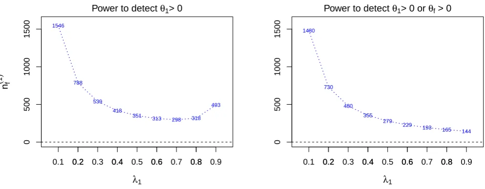
whereS∗ is the subset ofS and contains the specified subpopulations of interest. Take an example that ifS ={1, f}
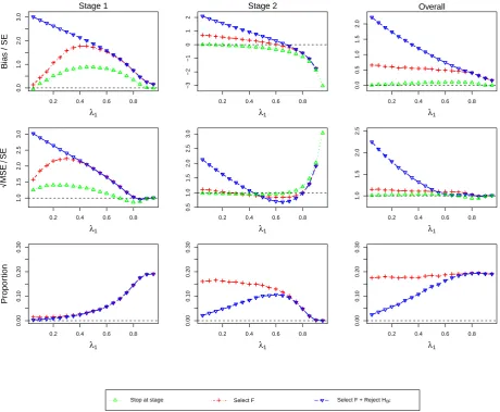
and S∗=S, Figure1 shows the resulting total sample sizes n(1)
f in a single-stage design, corresponding to different
prevalence values ofS1, under different definitions of power. The left panel is computed to have power1−βfor selecting
the subpopulation with the largest true effect and rejecting the corresponding null hypothesis, while the right panel considers any correct rejection. As the prevalenceλ1approaches 1,n
(1)
f increases again and becomes very large forλ1
close to 1 whereasn(1)f always decreases under the definition of power to detectθ1>0orθf >0. Since the effect sizes for
S1andFare close, it is difficult to select the correct subgroup and thus large sample sizes are needed. The reason that the
shown in this paper).
0.2 0.4 0.6 0.8
0
500
1000
1500
Power to detect θ1> 0
λ1
nf
(
1
)
1546
788
539 418
351 313
298 318 493
0.1 0.2 0.3 0.4 0.5 0.6 0.7 0.8 0.9 0.2 0.4 0.6 0.8
0
500
1000
1500
Power to detect θ1> 0 or θf > 0
λ1 1480
730
480 355
279
229 193
165 144
[image:8.595.64.561.128.322.2]0.1 0.2 0.3 0.4 0.5 0.6 0.7 0.8 0.9
Figure 1.The total sample sizes of the full populationF(n(1)f ) across prevalence rates ofS1(λ1) for two different definitions of power. The design is a
single-stage design with two subpopulations where the treatment effectsθ1andθ2forS1andS2are 0.5 and 0, respectively. The type-I error and power are
specified at 0.025 and80%.
3. Estimation Assessment
In this section we report a simulation study assessing the properties of MLEs. Note that in the reported figures different scales for the y-axes are used in order to highlight patterns.
3.1. Simulation Set-up
In our evaluations, we specify the family-wise error rate,α, as 0.025 and set the sample size for each scenario so that the power of the design is1−β = 80%. Our alternative hypothesis is that the treatment has an effect of 0.5 inS1while the
effect of the treatment is zero for all other subgroups. Therefore the power aims to detect the non-zero effect inS1(that
is to rejectH01) once the first subgroup is selected. The assumed common variance across subpopulations,σ2, is set to 1
and we use 1,000,000 simulation runs.
The designs we consider are: a single-stage design with two subpopulations(Design 1), a single-stage design with three subpopulations(Design 2), a two-stage design with two subpopulations and three subpopulations (Design 3and
Design 4, respectively), with anO0Brien Fleming (OBF) upper stopping boundary and a fixed lower boundary of zero is used. We calculate the stopping boundaries and the total sample sizes forF based on (2) and (3) for single-stage designs (and (5) and (6) for multi-stage designs). Based on these four designs, several scenarios are investigated altering the design features such as prevalence.
Denoteθˆas the naive MLE (that is not accounting for selection) for the parameterθ, thenθfˆ andθsˆ represent the MLEs for the treatment effect ofF and Ss, respectively. The estimates can be calculated byZ
(k)
s /Is(k)= ¯Ys,T(k)−Y¯s,C(k), where s∈ {1, f}in scenarios forDesign 1ands∈ {1,1 + 2, f}in scenarios forDesign 2. In multi-stage scenarios, the MLE estimates ofθfˆ andθˆ1are calculated byZs1:M/Is1:M = ¯Ys,T1:M −Y¯
1:M
s,C , wheres∈ {1, f}andM is the stage at which the
study stops.
We define bias as bias(θˆ) = E(θ)ˆ −θand the mean squared error (MSE), MSE(θˆ) = E((θˆ−θ)2) as performance measures
across different prevalence, a standardized scale is used in the assessments (readers are referred to Appendix A.6 for details on the standardization). In our subsequent evaluations we will consider three situations. Firstly, we consider the treatment effect estimator regardless of the population being selected or the hypothesis test being significant. Secondly we consider only the estimators of the selected populations which is expected to result inselection bias. The third situation considersreporting biasand for this we only consider only treatment effect estimates of the selected population if the corresponding hypothesis test is significant. Implicitly we are therefore considering that the outcome of a study is only reported (published) if it was significant. Note that in the evaluations to follow we refer to the selection bias asSelect Sw
and the reporting bias asSelect Sw +Reject H0w, wherewinSspecifies the population chosen through a selection rule.
3.2. Scenarios for Design 1
Scenarios here cover different prevalence values ofS1,λ1varying from 0.05 to 0.95 in increments of 0.05. We illustrate
the assessments for the scenarios under three configurations of different values ofθ1andθ2in Figure3-4. Their horizontal
axes are for the prevalence ofS1,λ1, and the vertical axes of the row-wise panels are for standardized bias, standardized
√
MSE and simulation proportions (%).
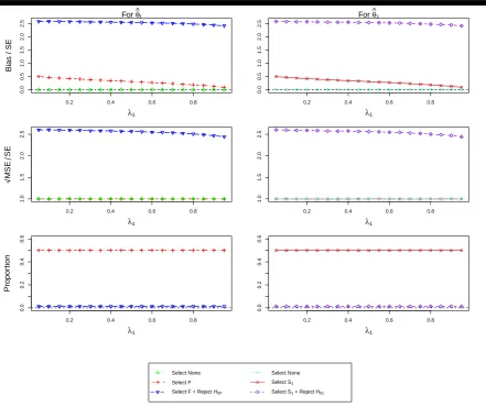
Figure2presents the estimation assessment ofθfˆ andθˆ1under the assumption ofθ1= 0andθ2= 0. As expected we
do not see any bias when no selection is undertaken as well as constant standardized MSE - a pattern that is repeated throughout all other simulations. Additionally the selection probability is constant at 50% due to the equal effect in both subgroups. The selection bias is largest when the prevalence in the subgroup is smallest with a matching pattern for the standardized MSE. The reporting bias and MSE follow the same pattern although at a markedly increased level.
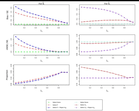
Figure 3considers the case whenθ1= 0.5and θ2= 0. Considering the selection probabilities first, we find that, as
per design, there is a 80% chance to select population 1 correctly and reject the corresponding hypothesis. The selection probability of the full population increases as the prevalence increases as the effect in the full population gets larger as the subpopulation contributes more towards it. At the same time the chance to also reject the hypothesis also increases. The selection and reporting bias in the full population estimate is largest when the prevalence in the subpopulation is smallest and then steadily decreases towards zero. The size of the bias is well over 0.5 standard errors for almost all prevalences and hence should be considered important although incorrect selection in itself is not very common in this case. For the full population the bias dominates the MSE and hence the MSE follows the same pattern.
Focusing attention on subpopulation 1, we find that bias is present, although it is of much smaller magnitude (selection bias at most 0.1 and reporting bias at most 0.35 standard errors) than for the full population (up to over 2 standard errors). The selection bias is maximised at a prevalence of around 0.75 while it is largest for a small prevalence for the reporting bias.
When both treatment groups have the same effect, θ1=θ2= 0.5(Figure 4) we observe that almost always the full
population is selected and only for large prevalences of the subpopulation (>50%) we obtain notable selection probability for the subpopulation (up to 20%). As a consequence of this we obtain no estimate of the bias and MSE for the subpopulation for low prevalences. The bias in the estimate in this population is potentially very large (>3 standard errors) but drops quickly towards zero as the prevalence increases. In this setting it is also notable, that the selection bias is virtually identical to the reporting bias as very large observed effects are necessary to select the subpopulation in the first place.
The patterns for the full population are somewhat more distinct as no bias is observed for small prevalences, since it is always the full population that is selected. The bias in this case is, however, very small even in the worst case situation (prevalence of around 0.75) where the reporting bias is less than 0.1 standard errors and the selection bias is even smaller.
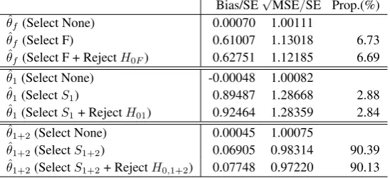
3.3. Scenarios for Design 2
Scenarios forDesign 2regard to select a population amongS1,S1+2andF under different configurations ofθ1,θ2and
0.2 0.4 0.6 0.8
0.0
0.5
1.0
1.5
2.0
2.5
For θ^f
λ1
Bias / SE
0.2 0.4 0.6 0.8
0.0
0.5
1.0
1.5
2.0
2.5
For θ^1
λ1
● ● ● ● ● ● ● ● ● ● ● ● ● ● ● ● ● ● ●
0.2 0.4 0.6 0.8
1.0
1.5
2.0
2.5
λ1
M
S
E
S
E
0.2 0.4 0.6 0.8
1.0
1.5
2.0
2.5
λ1
● ● ● ● ● ● ● ● ● ● ● ● ● ● ● ● ● ● ●
0.2 0.4 0.6 0.8
0.0
0.2
0.4
0.6
λ1
Propor
tion
0.2 0.4 0.6 0.8
0.0
0.2
0.4
0.6
λ1 Select None ● ● ●Select NoneSelect F Select SSelect SSelect F+ RejectH11+ RejectH+ RejectH000
● Select None
Select F Select F + Reject H0F
[image:10.595.90.532.84.454.2]Select None Select S1 Select S1 + Reject H01
Figure 2.(ForDesign 1,θ1= 0andθ2= 0) the standardized bias and standardized √
MSE of MLEsθˆf,θˆ1and the simulation proportions for different
circumstances against the prevalence of subpopulation 1,λ1.
given by
selectS1 if Z (k)
1 >max(Z (k)
f , Z
(k) 1+2)
selectS1+2 if Z (k)
1 ≯max(Z (k)
f , Z
(k)
1+2),and Z (k) 1+2> Z
(k)
f
selectF if Z1(k)≯max(Zf(k), Z1+2(k)),and Z1+2(k) < Zf(k),
(9)
This rule is one variant of the maximum statistic rule and sequentially decides which population to be selected. The results for other configurations of θ1,θ2 and θ3 are provided in Tables 3-5 in Appendix A.7. Note that for all the scenarios
simulations are run under the same stopping boundaries and sample sizes (n(1)f = 576) found based onDesign 2with the maximum statistics selection rule,θ1= 0.5, θ2= 0, θ3= 0and equal subgroup prevalence.
0.2 0.4 0.6 0.8
0.0
0.5
1.0
1.5
2.0
For θ^f
λ1
Bias / SE
0.2 0.4 0.6 0.8
0.0
0.1
0.2
0.3
For θ^1
λ1
● ● ● ● ● ● ● ● ● ● ● ● ● ● ● ● ● ● ●
0.2 0.4 0.6 0.8
1.0
1.5
2.0
λ1
M
S
E
S
E
0.2 0.4 0.6 0.8
0.80
0.90
1.00
1.10
λ1
● ● ● ● ● ● ● ● ● ● ● ● ● ● ● ● ● ● ●
0.2 0.4 0.6 0.8
0.00
0.10
0.20
0.30
λ1
Propor
tion
0.2 0.4 0.6 0.8
0.70
0.80
0.90
1.00
λ1 Select None ● ● ●Select NoneSelect F Select SSelect SSelect F+ RejectH11+ RejectH+ RejectH000
● Select None
Select F Select F + Reject H0F
[image:11.595.63.520.85.451.2]Select None Select S1 Select S1 + Reject H01
Figure 3.(ForDesign 1,θ1= 0.5andθ2= 0) the standardized bias and standardized √
MSE of MLEsθˆf,θˆ1and the simulation proportions for different
circumstances against the prevalence of subpopulation 1,λ1.
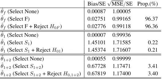
Bias/SE√MSE/SE Prop.(%)
ˆ
θf(Select None) -0.00186 0.99849
ˆ
θf(Select F) 0.96546 1.32104 3.74
ˆ
θf(Select F + RejectH0F) 1.31217 1.47472 2.91
ˆ
θ1(Select None) -0.00151 1.00004
ˆ
θ1(SelectS1) 0.09094 0.97526 88.58
ˆ
θ1(SelectS1+ RejectH01) 0.27068 0.87036 80.20
ˆ
θ1+2(Select None) -0.00118 0.99884
ˆ
θ1+2(SelectS1+2) 0.76128 1.19617 7.68
ˆ
θ1+2(SelectS1+2+ RejectH0,1+2) 1.02579 1.26021 6.47
Table 1.(ForDesign 2,θ1= 0.5,θ2= 0 andθ3= 0) Standardized bias and standardized
√
MSE of the MLEs where the prevalence rates of three subgroups are 1/3. In addition, Proportion (Prop.) stands for how often the corresponding
[image:11.595.165.437.549.673.2]0.2 0.4 0.6 0.8
−0.02
0.02
0.06
For θ^f
λ1
Bias / SE
0.2 0.4 0.6 0.8
0.0
1.0
2.0
3.0
For θ^1
λ1
● ● ● ● ● ● ● ● ● ● ● ● ● ● ● ● ● ● ●
0.2 0.4 0.6 0.8
0.95
1.00
1.05
1.10
λ1
M
S
E
S
E
0.2 0.4 0.6 0.8
1.0
1.5
2.0
2.5
3.0
3.5
λ1
● ● ● ● ● ● ● ● ● ● ● ● ● ● ● ● ● ● ●
0.2 0.4 0.6 0.8
0.80
0.85
0.90
0.95
1.00
λ1
Propor
tion
0.2 0.4 0.6 0.8
0.00
0.10
0.20
0.30
λ1 Select None ● ● ●Select NoneSelect F Select SSelect SSelect F+ RejectH11+ RejectH+ RejectH000
● Select None
Select F Select F + Reject H0F
[image:12.595.88.533.82.458.2]Select None Select S1 Select S1 + Reject H01
Figure 4.(ForDesign 1,θ1= 0.5andθ2= 0.5) the standardized bias and standardized √
MSE of MLEsθˆf,θˆ1and the simulation proportions for
different circumstances against the prevalence of subpopulation 1,λ1.
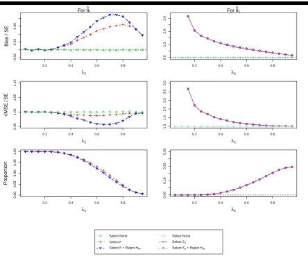
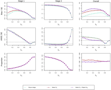
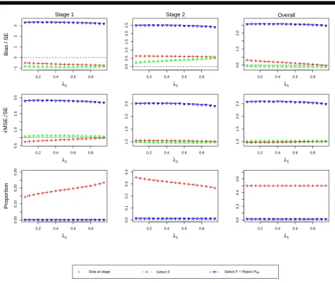
3.4. Scenarios for Design 3
The investigation presented here concerns Design 3, a two-stage design and we focus onθ1= 0.5andθ2= 0here while
the results for other configurations are given in Figures7-10of Appendix A.7.
Figure5shows the results of the estimator for the full population. The top row corresponds to standardized bias, middle row to standardized √MSE and the bottom row to the probability of selecting the full population. The first column is associated with the estimators that stop at Stage 1, the second considers only trials that reach Stage 2 while the final column corresponds to the estimator irrespective of when the trial was stopped. In addition to the selection bias and the reporting bias, we also consider the estimator irrespective of the reason for stopping (green triangle) in the figure.
the bias is smaller. It is noteworthy that, although substantial bias is exhibited under some situation, the probability of reaching these (e.g. selecting the full population and stopping at stage 1) are very rare. The standardized√MSE appears like that in standardized bias except for the second stage. In those exceptional cases, the MSE (for selection, reporting and regardless of selection) decreases at a different rate before inflating substantially at a prevalence of 0.8.
0.2 0.4 0.6 0.8
0.0
1.0
2.0
3.0
Stage 1
λ1
Bias / SE
0.2 0.4 0.6 0.8
−3
−2
−1
0
1
2
Stage 2
λ1
0.2 0.4 0.6 0.8
0.0
0.5
1.0
1.5
2.0
Overall
λ1
0.2 0.4 0.6 0.8
1.0
1.5
2.0
2.5
3.0
λ1
M
S
E
S
E
0.2 0.4 0.6 0.8
0.5
1.0
1.5
2.0
2.5
3.0
λ1
0.2 0.4 0.6 0.8
1.0
1.5
2.0
2.5
λ1
0.2 0.4 0.6 0.8
0.00
0.10
0.20
0.30
λ1
Propor
tion
0.2 0.4 0.6 0.8
0.00
0.10
0.20
0.30
λ1
0.2 0.4 0.6 0.8
0.00
0.10
0.20
0.30
λ1
[image:13.595.66.527.163.542.2]Stop at stage Select F Select F + Reject H0F
Figure 5.(ForDesign 3,θ1= 0.5andθ2= 0) standardized bias and MSE ofθˆfand simulation proportions for different circumstances at stopping stage 1, 2 and overall, against the prevalence of subpopulation 1,λ1.
Considering the findings for the estimator of the first subpopulation,θˆ1(Figure6), the results exhibit similar patterns in
for all prevalences and shows an inverted U-shape with a maximum bias of about 0.3 SEs for a prevalence of 0.6. Its MSE conditional on selection or no-selection appears different from that considering reporting before a prevalence of 0.7. The estimator thereafter performs similarly in MSE with a small U-shape under 1 SE.
0.2 0.4 0.6 0.8
0.0
0.5
1.0
1.5
2.0
2.5
Stage 1
λ1
Bias / SE ● ●●
●●●
● ●●●●● ●
● ●
● ●
●●
0.2 0.4 0.6 0.8
−3
−2
−1
0
Stage 2
λ1 ●● ●●●●● ●●●● ●●●
● ●
●
●
●
0.2 0.4 0.6 0.8
−0.1
0.1
0.3
0.5
Overall
λ1 ●●
●● ●● ●
●●●● ●●●● ●
● ●●
0.2 0.4 0.6 0.8
0.8
1.2
1.6
2.0
λ1
M
S
E
S
E
● ●●
● ●
● ●
● ●
● ●
● ●
● ●● ●
●●
0.2 0.4 0.6 0.8
1.0
1.5
2.0
2.5
3.0
λ1 ●● ●●●●● ●●●● ●●●●
● ●
● ●
0.2 0.4 0.6 0.8
0.9
1.0
1.1
1.2
1.3
λ1 ●● ●●●● ●●●●● ●
● ●
● ●●
●●
0.2 0.4 0.6 0.8
0.0
0.2
0.4
0.6
0.8
1.0
λ1
Propor
tion
0.2 0.4 0.6 0.8
0.0
0.2
0.4
0.6
0.8
λ1
0.2 0.4 0.6 0.8
0.70
0.75
0.80
0.85
0.90
λ1
● ● ●Select None Select F Select F+ RejectH0
[image:14.595.73.537.153.530.2]● Stop at stage Select S1 Select S1 + Reject H01
Figure 6.(ForDesign 3,θ1= 0.5andθ2= 0) standardized bias and MSE ofθˆ1and simulation proportions for different circumstances at stopping stage
1, 2 and overall, against the prevalence of subpopulation 1,λ1.
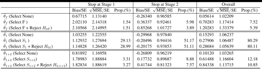
3.5. Scenarios for Design 4
Scenarios for Design 4 is the two-stage counterpart ofDesign 2 for selecting a population among S1, S1+2 and F
under different configurations ofθ1,θ2andθ3. The investigation here focus on assessing the MLEsθˆ1,θˆ1+2andθfˆ under
θ1= 0.5, θ2= 0, θ3= 0under the population selection rule given in the equation9. The results for other configurations of
θ1,θ2andθ3are provided in Tables6-8in Appendix A.7. All the simulations are run under the same stopping boundaries
Stop at Stage 1 Stop at Stage 2 Overall
Bias/SE √MSE/SE Prop.(%) Bias/SE √MSE/SE Prop.(%) Bias/SE √MSE/SE Prop.(%)
ˆ
θf(Select None) 0.67715 1.13140 -0.26340 0.96585 0.05614 1.02209
ˆ
θf(Select F ) 2.02110 2.14318 1.54 0.36337 0.92461 5.98 0.70283 1.17414 7.52
ˆ
θf(Select F + RejectH0F) 2.10568 2.14995 1.51 0.85268 1.01727 3.89 1.20283 1.33379 5.39
ˆ
θ1(Select None) 1.03255 1.22555 -0.29968 0.97840 0.15293 1.06237
ˆ
θ1(SelectS1) 1.12932 1.27694 29.13 -0.20496 0.94416 51.17 0.27906 1.06487 80.29
ˆ
θ1(SelectS1+ RejectH01) 1.14828 1.26420 28.99 -0.20175 0.93853 51.11 0.28684 1.05639 80.11
ˆ
θ1+2(Select None) 0.81892 1.16958 -0.26809 0.96219 0.10120 1.03265
ˆ
θ1+2(SelectS1+2) 1.78983 1.88884 3.31 0.17732 0.89687 8.88 0.61488 1.16604 12.18
ˆ
[image:15.595.75.526.88.208.2]θ1+2(SelectS1+2+ RejectH0,1+2) 1.82834 1.88619 3.27 0.41744 0.81323 7.57 0.84338 1.13715 10.85
Table 2.For Design 4,θ1= 0.5,θ2= 0 andθ3= 0) Standardized bias and standardized
√
MSE of the MLEs where the prevalence rates of three subgroups are 1/3. In addition, Proportion (Prop.) stands for how often the corresponding
circumstance occurs.
Table2shows the results of the estimators for the first subgroup, the combined subgroup and the full population. The standardized bias, standardized√MSE and simulation proportions are presented in the trials that stop at Stage 1, reach Stage 2 and are irrespective of which stopping stage.
Considering the trials irrespective of stopping, we observed the correct population is selected in the80%of simulations due to the design requirement of 80% power. The bias is found positive for all the overall estimators and varies widely (smallest at 0.05 and maximum up to 1.2 standard errors). The selection and reporting bias when selecting the correct population are the smallest (less than 0.3 standard errors), but larger when selecting the incorrect population (particularly for the full population). All the standardized MSE are larger than 1 standard errors but only up to a moderate size of around 1.3. While selecting the correct population or rejecting the null hypothesis the estimator for the first subgroup has a smaller standardized MSE (around 1.06 standard errors) than its counterparts.
The results at different stages show a contrary picture. More trials stop at stage 2 than at Stage 1 and each stage has a higher proportion of selecting the correct population (around30%and50%at Stage 1 and Stage 2, respectively). The bias is large at Stage 1. The selection and reporting bias are smaller when selectingS1(around 1.1 standard errors) than
those when selectingS1+2 orF (around 1.8 and 2, respectively). A moderate bias is observed at Stage 2 (up to 0.85
standard errors). In particular, the selection and reporting bias are found negative in the estimator for the first subgroup. The standardized MSE of all the estimators at Stage 1 are much larger than 1 SE but those at Stage 2 show the opposite pattern being less than 1 (between 0.8 and 1).
4. Discussions and concluding Remarks
In this paper we have discussed general design considerations for clinical trials with subpopulation selection and illustrate how such studies can be designed. Selection based on the maximum test statistics is only investigated throughout the paper. While this selection rule is simple and intuitive, it may not be optimal in certain circumstances. It makes sense to adopt the rule when some subgroup treatment effects have been identified as being positive and difference between test statistics across subgroups are reasonably large. However, when the test statistic forSsandF are close but the former is larger, applying this rule leads to ethical issues that selecting only part of the population rather than the whole population although they could benefit from the treatment. Therefore, other options for selection rules should be considered for similar situations and investigation.
difference is within a threshold) to be united so that the pooled population can continue to the next stage. Meanwhile, it also permits to select a population whose effect size is above a threshold plus the effect size from the others. This threshold perhaps can be viewed as the degree of efficacy consistency for further testing.
Another option that has been used in the context of treatment selection (e.g. [34,12]) is simply to select a population whose efficacy exceeds a certain value at stage 1. This selection rule was used in [12] and integrates population selection and hypothesis testing at the first stage. Their designs considering a prior ordering on underlying effect sizes of all individual subgroups somehow connect to ours where the target subpopulations for selection has a nested structure. It is noted that the mathematical expression ofpZ(1)
W,W
(·,·)in (1) will be different if the above selection rules are used.
In term of estimation we have assessed the bias of the MLE under various scenarios. We find that almost always bias is positive leading to an over-enthusiastic estimate of the true treatment effect. While for some settings the size of the bias can be viewed as negligible it can become large under other situations. The challenge clearly being that one will usually not know if one is in one of these extreme situations. Another observation we make is that although bias is introduced by selecting the population, the bias gets markedly increased (often more than doubled) when only significant results are reported highlighting the effect of reporting bias which may be even more problematic than the bias introduced by selection.
Our results suggest the MSE of the overall MLEs performs quite well (around 1 standard error) in many circumstances and scenarios. We find whether selecting the correct population or not impacts the size of MSE for the corresponding estimator. The extent can be more substantial when further reporting significant results. The same finding is even observed in the extreme scenario, where no correct population is defined because the underlying effect of each subgroup is assumed none.
In this work we only consider designs with normally distributed endpoints, although they can easily be extend to other types of endpoints via the efficient scores framework [35]. Moreover we assume that the subgroup prevalence is known although clearly specifying this parameter correctly in the design will be crucial for the designs operating characteristics. A consequence of the assumed known prevalence is that we only present the estimation assessment of the MLE where subgroup sample sizes are fixed according to the respective prevalence in designs. Further simulations (not shown), however, suggest that random sample sizes of populations only alter the findings marginally.
Future work will consider estimators that are unbiased (or have smaller bias) while maintaining comparable MSE. Conditional bias-adjusted estimator following the ideas in [24] appear most promising. One extension to the case of multiple-stage designs given the process continues to the final stage can be naturally achieved. However, whether the derived estimators have less MSE should be verified in further investigations.
References
1. Ondra T, Dmitrienko A, Friede T, Graf A, Miller F, Stallard N, Posch M. Methods for identification and confirmation of targeted subgroups in clinical
trials: a systematic review.Journal of Biopharmaceutical Statistics2016;26(1): 99-119.
2. Alosh M, Huque M, Bretz F, et al. Tutorial on statistical considerations on subgroup analysis in confirmatory clinical trials.Statistics in Medicine2016;
7(8): 889-894.
3. Lipkovich I, Dmitrienko A, D’Agostino R.B. Tutorial in biostatistics: data-driven subgroup identification and analysis in clinical trials.Statistics in Medicine2017;36(1): 136-196.
4. Placzek M, Friede T. Clinical trials with nested subgroups: Analysis, sample size determinatino and internal pilot studies.Statistical Methods in Medical
Research2017; first published date: March-14-2017, 10.1177/0962280217696116.
5. Spiessens B, Debois M. Adjusted significance levels for subgroup analyses in clinical trials.Contemporary Clinical Trials2010;20: 331-335.
6. Song Y, Chi G. A method for testing a prespecified subgroup in clinical trials.Statistics in Medicine2007;26(1): 3535-3549.
8. Graf A C., Posch Martin, Koening F. Adaptive designs for subpopulation analysis optimizing utility functions.Biometrical Journal2015;57(1): 76-89.
9. Jennison C, Turnbull B W.Group Sequential Methods with Applications to Clinical Trials.Chapman&Hall/CRC Boca Raton, FL, USA, 2000. 10. Bauer P, Kieser M. Combining different phases in the development of medical treatments within a single trial.Statistics in Medicine1999;18:
1833-1848.
11. Ghosh P, Liu L.Y., Senchaudhuri P., Gao P., Mehta C. Design and Monitoring of Multi-Arm Multi-Stage Clinical Trials.Biometrics2017; first published:
27 March 2017. DOI: 10.1111/biom.12687.
12. Magnusson B, Turnbull BW. Group sequential enrichment design incorporating subgroup selection.Statistics in Medicine2013;32(16): 2695-2754.
13. Jenkins M, Stone A, Jennison C. An adaptive seamless phase II/III design for oncology trials with subpopulation selection using correlated survival
endpoints.Pharmaceutical Statistics2011;10: 347-356.
14. Stallard N, Hamborg T, Parsons N, Frided T. Adaptive designs for confirmatory clinical trials with subgroup selection.Journal of Biopharmaceutical Statistics2014;24(1): 168-187.
15. Bauer P, Koenig F, Brannath W, Posch M. Selection and bias–Two hostile brothers.Statistics in Medicine2010;29(1): 1-13.
16. Shen L. An improved method of evaluating drug effect in a multiple dose clinical trial.Statistics in Medicine1999;20: 1913-1929.
17. Stallard N, Todd S, Whitehead J. Estimation following selection of the largest of two normal means.Journal of Statistical Planning and Inference2008;
138: 1629-1638.
18. Cohen A, Sackrowitz H. Two stage conditionally unbiased estimators of the selected mean.Statistics and Probability Letters1989;8: 273-278. 19. Bowden J, Glimm E. Unbiased estimation of selected treatment means in two-stage trials.Biometrical Journal2008;50(4): 515-527.
20. Sill M W, Sampson A R. Extension of a two-stage conditionally unbiased estimator of the selected population to the bivariate normal case.
Communications in Statistics - Theory and Methods2007;36(4): 801-813.
21. Carreras M, Brannath W. Shrinkage estimation in two-stage adaptive designs with midtrial treatment selection.Statistics in Medicine2013;32(10):
1677-1690.
22. Kimani P, Todd S, Stallard N. A comparison of methods for constructing confidence intervals after phase II/III clinical trials.Biometrical Journal2014;
56(1): 107-128.
23. Magirr D, Jaki T, Posch M, Klinglmueller F. Simultaneous confidence intervals that are compatible with closed testing in adaptive designs.Biometrika
2013;100(4): 985–996.
24. Stallard N, Todd S. Point estimates and confidence regions for sequential trials involving selection.Journal of Statistical Planning and Inference2005;
135: 402-419.
25. Brckner M, Titman A, and Jaki T. Estimation in multi-arm two-stage trials with treatment selection and time-to-event endpoint.Statistics in Medicine
2017; published online ahead of print.
26. Rosenkrankz G K. Bootstrap corrections of treatment effect estimates following selection.Statistics in Medicine2014;69: 220-227.
27. Kimani P, Todd S, Stallard N. Estimation after subpopulation selection in adaptive seamless trials.Statistics in Medicine2015;34(18): 2581-2601. 28. Wang Y, Leung D. Bias reduction via resampling for estimation following sequential tests.Sequential Analysis1997;16(3): 249-267.
29. Davison A, Hinkley D.Bootstrap Methods and Their Application.Cambridge University Press: Cambridge, UK, 1999.
30. Dmitrienko A, Tamhane A.C., Bretz F., editors.Multiple Testing Problems in Pharmaceutical Statistics.Chapamn&Hall/CRC biostatistics series, Boca Raton, 2010.
31. Marcus R., Peritz E., Gabriel K.R. On closed testing procedures with special reference to ordered analysis of variance.Biometrika1976;63(3): 655-660.
32. O’Brien P.C., Fleming T.R. A Multiple Testing Procedure for Clinical Trials.Biometrics1979;35(3): 549-556.
33. Bretz F, Koenig F, Brannath W, Glimm E, Posch M. Tutorial in Biostatistics - Adaptive designs for confirmatory clinical trials.Statistics in Medicine
2009;28: 1181-1217.
34. Magirr D., Jaki T., Whitehead J. A generalized Dunnett test for multi-arm multi-stage clinical studies with treatment selection.Biometrika2012;99:
494-501.
35. Whitehead J.The Design and Analysis of Sequential Clinical Trials.Revised 2nd edn. Wiley: Chichester, 1997.
A. Appendices
A.1. The derivations of Stopping Boundaries and Sample Size
Consider all the possible situations that lead to rejecting any individual null hypothesis, then the inequality (2) for searching critical values can be derived based on
α≥P rh [
w∈S
(ZW(1)> Cα, W =w)|H0
i
= X
w∈S
P rh(ZW(1)> Cα, W =w)|H0
i
= X
w∈S
Z ∞
Cα
pZ(1)
W,W
(zw(1), w;Θ0)dzw(1) (A.1)
and similarly (3) which can be used to find the total sample size is based on
1−β≥P rh(ZW(1)> Cα, W =w)|Ha i
=P rh(ZW(1)> Cα, W =w)|Ha i
= Z ∞
Cα
pZ(1)
W,W
(z(1)w , w;Θa)dz(1)w . (A.2)
For a multi-stage setting we begin equally by considering all situations that lead to rejecting any individual null hypothesis at any stages and find equation (5) as
α≥P rh [
w∈S
(ZW(1)> Cu1,α, W =w)|H0
i
+P r [
w∈S
(Cl1 < ZW(1)< Cu1,α, ZW1:2> Cu2,α, W =w)|H0
i
+. . .+P rh [
w∈S
(Cl1 < Z
(1)
W < Cu1,α, . . . , ClK−1 < Z
1:(K−1)
W < CuK−1,α, Z
1:K
W > CuK,α, W =w)|H0
i
=X
w∈S
(
P r h
(ZW(1)> Cu1,α, W =w)|H0
i +P r
h
(Cl1 < ZW(1)< Cu1,α, ZW1:2> Cu2,α, W =w)|H0 i
+. . .+P rh(Cl1 < ZW(1)< Cu1,α, . . . , ClK−1< ZW1:(K−1)< CuK−1,α, ZW1:K > CuK,α, W =w)|H0
i )
=X
w∈S
" Z ∞
Cu1,α
pZ(1)
W,W
(zw(1), w;Θ0)dzw(1)+ Z Cu1,α
Cl1
Z ∞
Cu2,α
pZ(1)
W,W
(zw(1), w;Θ0)·pw,2|1(z1w:2|z
(1)
w ;Θ0)dzw1:2dz
(1)
w
+. . .+ Z Cu1,α
Cl1
· · ·
Z CuK−1,α
ClK−
1
Z ∞
CuK ,α pZ(1)
W,W
(zw(1), w;Θ0)·pw,2|1(z1w:2|z
(1)
w )· · · ·
· · ·pw,K|K−1(z1w:K|z
1:(K−1)
w )dz
1:K
w dz
1:(K−1)
w · · ·dz
(1)
w #
=X
w∈S
( K X
k=1
hZ . . .
Z
Ak
pZ(1)
W,W
(z(1)w , w;Θ0)· 1
Y
m=k
pw,m|m−1(z1w:m|z
1:(m−1)
w ;Θ0)
dzw1:k. . . dz
(1)
w i
)
Similarly the inequality (6) is found as
1−β≤P rh(ZW(1)> Cu1,α, W =w)|Ha i
+P r
(Cl1 < Z
(1)
W < Cu1,α, ZW1:2> Cu2,α, W =w)|Ha i
+. . .+P rh(Cl1 < ZW(1)< Cu1,α, . . . , ClK−1 < Z
1:(K−1)
W < CuK−1,α, Z
1:K
W > CuK,α, W =w)|Ha
i
=P r h
(ZW(1)> Cu1,α, W =w)|Ha i
+P r h
(Cl1 < ZW(1)< Cu1,α, ZW1:2> Cu2,α, W =w)|Ha i
+. . .+P rh(Cl1 < Z
(1)
W < Cu1,α, . . . , ClK−1 < Z
1:(K−1)
W < CuK−1,α, Z
1:K
W > CuK,α, W =w)|Ha
i
= Z ∞
Cu1,α
pZ(1)
W,W
(z(1)w , w;Θa)dzw(1)+ Z Cu1,α
Cl1
Z ∞
Cu2,α
pZ(1)
W,W
(zw(1), w;Θa)·pw,2|1(zw1:2|z(1)w ;Θa)dzw1:2dzw(1)
+. . .+ Z Cu1,α
Cl1
· · ·
Z CuK−1,α
ClK−1
Z ∞
CuK ,α pZ(1)
W,W
(z(1)w , w;Θa)·pw,2|1(z1w:2|z
(1)
w )· · · ·
· · ·pw,K|K−1(zw1:K|z
1:(K−1)
w )dz
1:K
w dz
1:(K−1)
w · · ·dz
(1) w = K X k=1 hZ . . . Z Ak
pZ(1)
W,W
(zw(1), w;Θa)·
1
Y
m=k
pw,m|m−1(zw1:m|z
1:(m−1)
w ;Θa)
dz1w:k. . . dz
(1)
w i
. (A.4)
A.2. Design 1- single-stage designs with two subgroups
Given the index set for population selectionS={1, f}, the joint distribution of two test statisticsZ1(1)andZf(1)is
Z1(1)
Zf(1) !
=N
θ1I
(1) 1
θfI
(1) f ! , 1 √ λ1 √
λ1 1
!!
.
Let the selected test statistic and the selected population index be ZW(1) and W. Both are random variables and particularlyW = 1 or f refers to whether subpopulation1 or the full population is chosen. The joint density of ZW(1)
andW,pZ(1)
W,W
(zw(1), w), is equal topZ(1)
w (z (1)
w )·p(W =w|Zw(1)=zw(1)). IfZw(1)=zw(1), thenW =wif Zu(1)< zw(1) for
allu6=w. To express the probability for this event it is required to find the distribution ofZu(1)|Z
(1)
w =z
(1)
w . AsZ
(1)
u and
Zw(1)are correlated, we need to exploit a property of conditional densities of the multivariate normal distribution (refer to
Section 0.3 in [36]. Applying this fact it follows that
Zf(1)|Z1(1)=z1(1) ∼ NθfIf(1)+pλ1(z (1) 1 −θ1I
(1)
1 ),1−λ1
,
and
Z1(1)|Zf(1)=z(1)f ∼ Nθ1I (1) 1 +
p λ1(z
(1)
f −θfI
(1)
f ),1−λ1
.
Then the densities of the joint distribution ofZW(1)andW are
pZ(1)
W,W
(z(1)w , w;Θ) =φ(z(1)w −θwIw(1))Φ
z(1)w −θuIu(1)−
√
λ1(z (1)
w −θwI
(1)
w )
√
1−λ1
, s6=u∈ {1, f}.
As a result, (2) for critical valueCαand (3) for the total sample size ofF are respectively as follows:
α ≥
Z ∞
Cα
pZ(1)
W,W
(z(1)1 ,1;Θ0)dz (1) 1 +
Z ∞
Cα
pZ(1)
W,W
(z(1)f , f;Θ0)dz (1)
f ,
1−β ≤
Z ∞
Cα
pZ(1)
W,W
(z(1)1 ,1;Θa)dz
A.3. Design 2- single-stage designs with three subgroups
Define the index set for population selection asS={1,1 + 2, f}, the joint distribution of three test statisticsZ1(1),Z1+2(1)
andZf(1)is then
Z1(1)
Z1+2(1)
Zf(1) =N
θ1I (1) 1
θ1+2I (1) 1+2
θfIf(1) ,
1 q λ1
λ1+λ2
√
λ1
q λ1
λ1+λ2 1
√
λ1+λ2
√
λ1
√
λ1+λ2 1
,
where the entries of the above covariance matrix are obtained by
cov(Z1(1), Z1+2(1) ) = I
(1) 1
I1+2(1)
, cov(Z1(1), Zf(1)) =I
(1) 1
If(1)
, cov(Z1+2(1) , Zf(1)) = I
(1) 1+2
If(1) .
To derive the densities of the joint distribution ofZW(1) andW, the conditional densities ofZu(1), Zv(1)|Zw(1)=zw(1)for
all u, v6=w need to be found. Using the gaussian identity about the conditional densities of the multivariate normal distribution, they are
(Z1+2(1) , Zf(1))T|Z1(1)=z(1)1 ∼ N(µ1+2,f,Σ1+2,f), (A.5) (Z1(1), Zf(1))T|Z1+2(1) =z1+2(1) ∼ N(µ1,f,Σ1,f), (A.6) (Z1(1), Z1∪2(1))T|Zf(1)=z(1)f ∼ N(µ1+2,Σ1,1+2), (A.7)
where
µ1+2,f =
θ1+2I
(1) 1+2+
q λ1
λ1+λ2(z
(1) 1 −θ1I
(1) 1 )
θfIf(1)+√λ1(z (1) 1 −θ1I
(1) 1 )
,
µ1,f =
θ1I
(1) 1 +
q λ1
λ1+λ2(z
(1)
1+2−θ1+2I (1) 1+2)
θfIf(1)+√λ1+λ2(z (1)
1+2−θ1+2I (1) 1+2)
,
µ1,1+2=
θ1I (1) 1 +
√
λ1(z (1)
f −θfI
(1)
f )
θ1+2I (1) 1+2+
√
λ1+λ2(z (1)
f −θfI
(1)
f )
!
,
and
Σ1+2,f =
1 √λ1+λ2
√
λ1+λ2 1
! − q λ1
λ1+λ2
√ λ1 q λ1
λ1+λ2
√
λ1
,
Σ1,f =
1 √λ1
√
λ1 1
! − q λ1
λ1+λ2
√
λ1+λ2
q
λ1
λ1+λ2
√
λ1+λ2
,
Σ1,1+2=
1 q λ1
λ1+λ2
q
λ1
λ1+λ2 1
−
√
λ1
√
λ1+λ2
! √
λ1
√
λ1+λ2
,
As a result, the joint densities ofZW(1)andW with different elements ofW are
pZ(1)
W,W
(zw(1), w;Θ) =φ(zw(1)−θwIw(1))Ψu,v
z(1)w , zw(1);Θ
whereΨu,v(·,·;Θ)is the conditional cumulative distribution function of the bivariate normal distribution corresponding to (A.5) or (A.6) or (A.7). Consequently, (2) for critical valueCαis as follows:
α≥
Z ∞
Cα
pZ(1)
W,W
(z(1)1 ,1;Θ0)dz (1) 1 +
Z ∞
Cα
pZ(1)
W,W
(z(1)1+2,1 + 2;Θ0)dz (1) 1+2+
Z ∞
Cα
pZ(1)
W,W
(zf(1), f;Θ0)dz (1)
f .
And the equation which searching sample sizes depends on is the same as that in Section A.2.
A.4. The derivations of conditional densities (multi-stage designs with multiple subgroups)
The conditional densities in (4) are derived from the definition of the test statistic and the distributional properties. Given
Swbeing chosn (w∈ S), the test statistics based on the accumulated data at the end of stagek,Zw1:k, can also be written
as
Zw1:k = k X
i=1
s Iw(i) I1:k w
Zw(i)= k X
i=1
s n(wi) n1:k w
Zw(i)= s
Iw1:(k−1) I1:k
w
Zw1:(k−1)+ s
Iw(k) I1:k w
Zw(k)= s
n1w:(k−1) n1:k
w
Zw1:(k−1)+ s
n(wk) n1:k w
Zw(k),
Then,
Zw1:k−
s
n1w:(1−k) n1:k
w
Zw1:(1−k) ∼ N
s n(wk) n1:k w
Iw(k)θw,n
(k)
w n1:k
w
,
so that the conditional distribution ofZw1:kgivenZ
1:(k−1)
w =z
1:(k−1)
w follows
Zw1:k|Z
1:(k−1)
w =z
1:(k−1)
w ∼ N
s
n1w:(k−1) n1:k
w
z1w:(k−1)+ s
n(wk) n1:k w
Iw(k)θw, n(wk) n1:k w
.
The conditional densities with different population selection are
pw,k|k−1(Zw1:k|Zw1:(k−1)=z1w:(k−1);Θ) = 1 q
n(wk)
n1:k
w
φ Z1:k
w −
q
n1w:(1−k)
n1:k
w
z1w:(k−1)− q
n(wk)
n1:k
w
Iw(k)θw
q
n(wk)
n1:k
w
, (A.8)
In general, n1w:(k−1)
n1:k
w
=λw+(k−2)
λw+(k−1)and
n(wk)
n1:k
w
= 1
λw+(k−1), whereλwis the prevalence ofSwin the full populationF, where w∈ S.
A.5. Design 3- two-stage designs with two subgroups
Given the index set for population selectionS={1, f}, Equation (5) for critical values is:
α≥
Z ∞
Cu1,α
pZ(1)
W,W
(z1(1),1;Θ0)dz (1) 1 +
Z Cu1,α
0
Z ∞
Cu2,α
pZ(1)
W,W
(z(1)1 ,1;Θ0)·pw,2|1(z11:2|z (1)
1 ;Θ0)dz11:2dz (1) 1 +
Z ∞
Cu1,α
pZ(1)
W,W
(z(1)f , f;Θ0)dz (1)
f +
Z Cu1,α
0
Z ∞
Cu2,α
pZ(1)
W,W
(zf(1), f;Θ0)·pw,2|1(z1f:2|z
(1)
f ;Θ0)dzf1:2dz
(1)
f ,
where Cu1,α and Cu2,α are upper critical values at stage 1 and 2. Moreover, Cu1,α=COBF(2, α)
√
2 and Cu2,α=