Extremal dependence of random scale constructions

Extremal dependence of random scale constructions

Sebastian Engelke

, Thomas Opitz

, and Jennifer Wadsworth

1_{Research Center for Statistics, University of Geneva, Boulevard du Pont d’Arve 40, 1205 Geneva, Switzerland,} [email protected]

2

Biostatistics and Spatial Processes, INRA, 84914, Avignon, France,[email protected]

3_{Department of Mathematics and Statistics, Fylde College, Lancaster University, LA1 4YF, UK,}

[email protected]

April 26, 2019

Abstract

A bivariate random vector can exhibit either asymptotic independence or dependence between the largest values of its components. When used as a statistical model for risk assessment in fields such as finance, in-surance or meteorology, it is crucial to understand which of the two asymptotic regimes occurs. Motivated by their ubiquity and flexibility, we consider the extremal dependence properties of vectors with a random scale construction (X1, X2) = R(W1, W2), with non-degenerateR > 0 independent of (W1, W2). Focusing on the presence and strength of asymptotic tail dependence, as expressed through commonly-used summary parame-ters, broad factors that affect the results are: the heaviness of the tails of R and (W1, W2), the shape of the support of (W1, W2), and dependence between (W1, W2). WhenRis distinctly lighter tailed than (W1, W2), the extremal dependence of (X1, X2) is typically the same as that of (W1, W2), whereas similar or heavier tails for

R compared to (W1, W2) typically result in increased extremal dependence. Similar tail heavinesses represent the most interesting and technical cases, and we find both asymptotic independence and dependence of (X1, X2) possible in such cases when (W1, W2) exhibit asymptotic independence. The bivariate case often directly ex-tends to higher-dimensional vectors and spatial processes, where the dependence is mainly analyzed in terms of summaries of bivariate sub-vectors. The results unify and extend many existing examples, and we use them to propose new models that encompass both dependence classes.

Keywords: copula, extreme value theory, residual tail dependence, tail dependence.

MSC2010: 60G70, 60E05, 62H20

1

Introduction

A rich variety of bivariate dependence models have a pseudo-polar representation

(X1, X2) =R(W1, W2), R >0, independent of (W1, W2)∈ W ⊆R2, (1)

where we term R the radial variable, assumed to have a non-degenerate distribution, and (W1, W2) the angular

variables. Indeed, many well-known copula families, including the elliptical, Archimedean, Liouville, and multi-variate Pareto families have such a representation. In this work, our focus is on the upper tail dependence of such constructions. In particular, we examine whether a given (X1, X2) displays asymptotic dependence or asymptotic

independence, and the strength of dependence within these classes. Our results are particularly useful for construct-ing new models with properties that reflect the challenges of real data in, for instance, finance, meteorology and hydrology. Specifically, it is often ambiguous whether data should be modeled using an asymptotically dependent or asymptotically independent distribution, and most families of distributions only exhibit one type of dependence. A vector (X1, X2) withXj∼FXj is said to display asymptotic dependence if the limit

χX = lim

q→1P{X1≥F −1

X1(q), X2≥F −1

X2(q)}/(1−q) (2)

coefficient, and the value ofχX∈(0,1] summarizes the strength of the dependence within the class of asymptotically

dependent variables. Under asymptotic independence, a more useful summary is the rate at which the convergence to zero in equation (2) occurs, and a widely satisfied assumption (Ledford and Tawn,1997) is

P{X1≥FX−11(q), X2≥F −1

X2(q)}=`(1−q)(1−q)

1/ηX_{, η}

X∈[0,1], (3)

where ` : [0,1] →<sub>R</sub>+ is slowly varying at zero, i.e., lims→0`(sx)/`(s) = 1, x >0. The parameter ηX is termed

the residual tail dependence coefficient; positive and negative extremal association are indicated respectively by

ηX ∈(1/2,1] andηX ∈[0,1/2), whilst asymptotically dependent variables haveηX= 1 andχX= limq→1`(1−q).

A value ofηX= 0 means that the left-hand side of (3) decays faster than any power of 1−q, whilst if the left-hand

side is exactly zero for someq <1, we say thatηX is not defined.

Our particular interest in the extremal dependence of constructions of the form (1) stems not from their novelty, but from their ubiquity and flexibility. As mentioned, (1) already encompasses many well-known families, and moreover these families display different types of extremal dependence, which may be determined by the distribution ofR, the distribution of (W1, W2), or its supportW. There is a large body of literature that treats either individual

constructions of the form (1), or a particular subset of these constructions whereRor (W1, W2) have certain specified

properties; this literature will be reviewed in Section4. Our aim is to bring this scattered treatment together and more systematically characterize how the extremal dependence of (X1, X2) is determined by the properties ofRand

(W1, W2). By understanding which facets of the construction lead to different dependence properties, we are able

to determine dependence models that can capture both types of extremal dependence within a single parametric family; the recent proposals in Wadsworth et al.(2017),Huser et al.(2017) andHuser and Wadsworth(2018) are specific examples of this.

A broad split in representations of type (1) is the dimension of W, the support of (W1, W2). The most

com-mon case in the literature is that W is a one-dimensional subset ofR2, such as the unit sphere defined by some

norm or other homogeneous function. Examples include the Mahalanobis norm (elliptical distributions), L1 norm

(Archimedean and Liouville distributions), orL∞norm (multivariate Pareto distributions). On top of the support W, to obtain distributions within a particular family,Ror (W1, W2) may be specified to have a certain distribution.

WhereW is two-dimensional, it may sometimes be reduced to the one-dimensional case by redefining R, such as in the Gaussian scale mixtures of Huser et al. (2017); other times, such as for the scale mixtures of log-Gaussian variables in Krupskii et al.(2016), or the model presented inHuser and Wadsworth(2018), this cannot be done. Where W is two-dimensional, the possible constructions stemming from (1) form an especially large class, since (W1, W2) can itself have any copula. In this case, we focus on how the multiplication by R changes the extremal

dependence of (W1, W2), summarized by the coefficients (χW, ηW), to obtain the extremal dependence of the

mod-ified vector (X1, X2) in terms of its coefficients (χX, ηX). The marginal distributions of (W1, W2) andRwill play a

crucial role, since, intuitively, the heavier the tail ofR the more additional dependence is introduced in the vector (X1, X2).

As we are focused on the upper tail of (X1, X2), we henceforth assume (W1, W2) ∈ R2+; by the invariance

of copulas to monotonic marginal transformations, this also covers random location constructions of the form (Y1, Y2) =S+ (V1, V2),S∈R, (V1, V2)∈ V ⊆R2. For simplicity of presentation, we will often make the restriction

that W1 andW2 have the same distribution, with comments on relaxations of this assumption given in Section6.

Furthermore, whilst our focus on the bivariate case permits simpler notation, many of the results are directly applicable to the bivariate margins of multivariate and spatial models, whose extremal dependence is typically analyzed in terms of the coefficients (2) and (3). Examples are given in Section4, with further comment on higher dimensions in Section6.

There is no widely recognized standard for ordering univariate tail decay rates from the slowest to the fastest, although a broad characterization is given by the three domains of attraction of the maximum. We say that the random variable R is in the max-domain of attraction (MDA) of a generalized extreme value distribution if there exists a functionb(t)>0 such that ast→r?_{= sup{r: P(R≤r)<1},}

P(R≥t+r/b(t))/P(R≥t)→(1 +ξr)−1/ξ+ , r≥0,

for some ξ ∈ R, where a+ = max(a,0). The cases ξ > 0, ξ = 0, ξ < 0 define respectively the Fr´echet, Gumbel

We begin in Section2 by presenting results concerning the tail dependence of construction (1) according to the tail behavior ofR and the shape ofW, in the case where it is a one-dimensional support defined through a norm. We then characterize various cases whereW is two-dimensional, according to the behavior of bothRand (W1, W2),

in Section3. Section4is devoted to literature review and framing a large number of existing examples in terms of our general results, whilst Section5 illustrates the properties of some new examples inspired by the developments in the manuscript. In Section6we comment on generalizations and conclude. Proofs are presented in Section7.

1.1

Terminology and notation

For a random variable Q, we define its survival function FQ(q) = P(Q ≥ q), and distribution function FQ(q) =

1−FQ(q). If Q represents a bivariate random vector Q = (Q1, Q2), we denote the minimum of its margins by

Q∧=Q1∧Q2. For two functionsf andgwithg(x)6= 0 for valuesxabove some threshold valuex0, we writef ∼gif

f(x)/g(x)→1, where the limit is considered forx→ ∞if not stated otherwise. Similarly, we writef(x) =o(g(x)) to indicate that f(x)/g(x)→0. The convolution ofX ∼FX and Y ∼FY is denotedFX? FY =FX+Y. We recall

definitions of upper tail behavior classes for a random variableX with distributionF. Key tail parameters for these classes may be given as subscript, such as in ETα to refer to exponential-tailed distributions with rate α, but we

may omit the subscript if the specific value of the parameter is not of interest.

Definition 1(Light-, heavy- and superheavy-tailed distributions). The distributionF isheavy-tailedifexp(λx)F(x)→ ∞asx→ ∞, for anyλ >0. Further,F is superheavy-tailedif F(exp(·))is heavy-tailed. If F is not heavy-tailed, it is light-tailed.

Definition 2(Regularly varying functions and distributions (RV0_αand RV∞_α)). A measurable functiongisregularly varying at infinity or at zero with index α∈_Rif g(tx)/g(t)→xα _{ast→ ∞ ort →0 respectively for any x >0.}

We writeg∈RV∞_α org∈RV0_αrespectively. Ifα= 0, theng is said to be slowly varying. A probability distribution

F with upper endpointx?_{=∞is regularly varying with indexα≥0 ifF ∈RV}∞

−α. Ifx?<∞, thenF is regularly

varying atx? with indexαif F(x?− ·)∈RV0_α.

Definition 3 (Exponential-tailed distributions (ETα, ETα,β)). The distribution F with upper endpoint x? =∞

is exponential-tailed with rate α ≥ 0 if for any x > 0, F(t+x)/F(t) → exp(−αx), t → ∞. If α > 0 and

F(x) =r(x) exp(−αx),r∈RV∞_β, we writeF ∈ETα,β.

By definition,F ∈ETαwithα≥0 if and only ifF(log(·))∈RV∞−α. The class ETα,β withβ >−1 is referred to as

gamma-tailed distributions. Another important subclass of ETαare the convolution-equivalent distributions.

Definition 4 (Convolution-equivalent distributions (CEα)). The distribution F is convolution equivalent with

index α≥0 if F ∈ETα andF ? F(x)/F(x)→ 2

R∞

−∞exp(αx)F(dx)<∞. We writeF ∈CEα. We refer to the

classCE0 as subexponential distributions.

Definition 5 (Weibull- and log-Weibull tailed distributions (WTβ, LWTβ)). The distributionF is Weibull-tailed

with indexβ >0 if there exist α >0, γ∈R, and r∈RV∞γ such thatF(x)∼r(x) exp(−αxβ). F is

log-Weibull-tailedwith indexβ >0 if F(exp(·))∈WTβ.

We remark that some authors define heavy tails to be synonymous with regularly varying tails for which the tail indexα >0 (e.g.Resnick,2007). The definition that we use is broader, and includes distributions such as the log-Gaussian, as well as regularly varying tails. In practice, all of the heavy tailed distributions that we treat belong to the class of subexponential distributions, CE0.

2

Constrained angular variables

We focus firstly on the case whereW is defined by a normν; specifically letW={(w1, w2)∈R2+:ν(w1, w2) = 1}.

Other types of constrained spaces may sometimes be of interest, but norm spheres are a common restriction, and this focus allows greater generality in other aspects. In particular, all components of the vector are bounded in absolute value when the value of the norm is fixed. We examine the extremal dependence based on the heaviness of the tail ofR. Because the (W1, W2) are bounded, and subject to additional mild assumptions, we can classifyR

according to its MDA in this section.

The case whereR belongs to the Fr´echet MDA is the least delicate: as long as Rhas a much heavier tail than each of (W1, W2), results do not depend strongly on other considerations. No equality in distribution is assumed

betweenW1, W2in this case. WhenRis in the Gumbel or negative Weibull MDA, the shape of the normνbecomes

2.1

Radial variable in Fr´

echet MDA

Many of the most familiar results in the literature on extremal dependence concern the case when R is in the Fr´echet MDA; this is equivalent to regular variation of the tail of R, namely FR∈RV∞−1/ξ, ξ >0, whereα= 1/ξ

is called the tail index. A classical example of this is the (multivariate) Pareto copula, which can be constructed as in equation (1) with R standard Pareto, andW ={(w1, w2)∈R2+ : max(w1, w2) = 1} (Ferreira and de Haan,

2014). Pareto copulas can be identified with so-called extreme value copulas, which arise as the limiting copulas of suitably normalized componentwise maxima; see e.g. Rootz´en et al. (2018). The next result provides the general form of the tail dependence coefficient for these models.

Proposition 1 (Rin Fr´echet MDA). Let FR∈RV∞−α,α≥0, P(W1>0) =P(W2>0) = 1, and E(Wjα+ε)<∞,

j= 1,2, for someε >0. ThenηX= 1, and

χX =E[min{W1α/E(W α 1), W

α 2/E(W

α

2)}]. (4)

Remark 1. When FR(r) ∼ Cr−α for some C > 0, then the condition E(Wjα+ε) < ∞ can be replaced by

E(Wα

j )<∞, by Lemma 2.3 of Davis and Mikosch(2008).

Remark 2. The condition E(W_jα+ε) <∞ is guaranteed when W is the unit sphere of a norm ν; Proposition1

notably also covers the case where (W1, W2)∈R2+.

Remark 3. The result includes the caseα= 0, although the tail of such an R is too heavy to be in any domain of attraction. In this case, χX = 1, representing perfect upper tail dependence. This case is discussed further in

Section3.1.

From (4), we observe that asymptotic dependence arises since P{min(Wα

1/E(W1α), W2α/E(W2α))>0} = 1. If

the conditions of the Proposition were relaxed to P(W1 >0),P(W2 >0) >0, then it is possible that for α >0,

P{min(Wα

1/E(W1α), W2α/E(W2α))>0} = 0 which would yield asymptotic independence, and then ηX would not

be defined. The Fr´echet case with one-dimensionalW is therefore very restricted in its capacity to represent varied asymptotically independent behaviors. A more complete description of tail dependence is given by the exponent function, defined as

VX(x1, x2) = lim

t→∞t[1−P(X1≤F −1

X1{1−1/(tx1)}, X2≤F −1

X2{1−1/(tx2)})], x1, x2>0. (5)

Small modifications to Proposition1 yield

VX(x1, x2) = E [max{W1α/(E(W α

1)x1), W2α/(E(W α

2)x2)}]. (6)

The link between χX and VX(1,1) can be obtained simply by inclusion-exclusion arguments; in particular since

min(a, b) =a+b−max(a, b),χX= 2−VX(1,1). With the assumptions of Proposition1, the random vector (X1, X2)

satisfies the condition of multivariate regular variation in the sense that limt→∞(1−F(tx1, tx2))/(1−F(t, t)) has

finite positive limit for anyx1, x2>0; seeResnick(1987, Section 5.4.2) for details about the notion of multivariate

regular variation. To abstract away from the marginal distributions inF, we can replacetxjby the quantile function

F_Xj−1(1−1/(txj)),j = 1,2, in this limit. If the latter exists, it is given byV(x1, x2)/V(1,1), and existence of the

limit is equivalent to Equation (5). While many of the specific examples of random scale constructions presented in this paper satisfy Equation (5), our general results focus on the behavior along the diagonal wherex1=x2, and

we do not aim to provide specific statements about off-diagonal behavior withx16=x2.

Example 1. Let FR ∈ RV∞−1, i.e., α = 1, and (W1, W2) ∈ W = {(w1, w2) ∈ [0,1]2 : w1+w2 = 1}. Taking

(W1, W2) = (W,1−W) then W ∈ [0,1], with E(W) = 1/2, is the random variable described by the L1 spectral

measure (e.g. Coles and Tawn, 1991). A simple example is the Gumbel or logistic spectral measure, which has Lebesgue density

h(w) ={w(1−w)}1/θ−2{w1/θ+ (1−w)1/θ}θ−2(1−θ)/(2θ) θ∈(0,1), (7)

χX = 2−2θ andVX(x1, x2) = (x −1/θ 1 +x

0.0 0.2 0.4 0.6 0.8 1.0

0.0

0.2

0.4

0.6

0.8

1.0

0 b1 b2 1

0

ζ

1

0.0 0.2 0.4 0.6 0.8 1.0

0.0

0.2

0.4

0.6

0.8

1.0

θ = 1.2

0.0 0.2 0.4 0.6 0.8 1.0

0.0

0.2

0.4

0.6

0.8

1.0

θ = 5

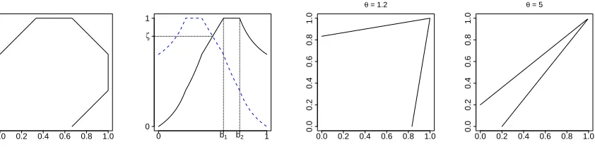
Figure 1: Left: the unit sphere for a particular normν; centre-left: illustration ofτ(z) (solid line) andτ(1−z) (dashed line) for the sameν. Centre-right and right: illustration of the unit sphere ofν(x, y) =θmax(x, y)+(1−θ) min(x, y) for two different values ofθ.

2.2

Radial variable in Gumbel MDA

Suppose thatRis in the Gumbel MDA, with upper endpointr?_{∈(0,∞] i.e.,}

lim

t→r?FR(t+r/b(t))/FR(t) =e

−r_,

whereb(t) is termed the auxiliary function. Such distributions can be expressed as

FR(r) =c(r) exp

−

Z r

z

b(t)dt

, (8)

where z < r < r?, c(r) → c > 0 as r → r?, and a = 1/b is absolutely continuous with density a0 satisfying limt→r?a0(t) = 0 (e.g.Embrechts et al.,2013, Chapter 3.3). Several distributions in this domain have mass on_R−,

but we suppose here thatR is conditioned to be positive, which does not affect the tail behavior. If r? =∞, we also have (Hashorva,2012) that for anyλ >1, ρ∈R,

lim

r→∞(rb(r)) ρ_F

R(λr)/FR(r) = 0. (9)

Notation and assumptions for (W1, W2)

Suppose that W1 d

=W2 d

= W ∈[0,1] andν(W1, W2) = 1. To this end, we assume thatν is a symmetric norm,

i.e.,ν(x, y) =ν(y, x), and scaled to satisfyν(x, y)≥max(x, y), such that the unit sphere ofν is contained in that of max, withν(b,1−b) =b for someb ≥1/2. Let τ(z) =z/ν(z,1−z) = 1/ν(1,1/z−1). The random variable

Z=W1/(W1+W2)∈[0,1] has distribution symmetric about 1/2, and satisfies

(W1, W2) = (Z,1−Z)/ν(Z,1−Z) = (τ(Z), τ(1−Z)). (10)

Define Iν = [b1, b2]⊆[1/2,1] as the interval such that τ(z) = 1 for all z ∈Iν, andτ(z)<1 forz 6∈Iν, and write

τ(z) =τ1(z) forz∈[0, b1],τ(z) = 1 forz∈[b1, b2], andτ(z) =τ2(z) forz∈[b2,1], withτ1strictly increasing and

τ2 strictly decreasing. Figure 1 illustrates τ for a particular ν; further illustrations are given in Appendix C. We

assume further that

(Z1): Z has a Lebesgue density,fZ, positive everywhere on (0,1), and that its survival function is regularly varying

at 1, withFZ(1− ·)∈RV0αZ,αZ >0,

and make the following mild regularity assumptions on the norm,ν, or equivalently τ:

(N1): The function τ is twice (piecewise) continuously differentiable except for finitely many points, at which we only require existence of left and right derivatives of first and second order.

In practice, (N1) and (N2) are satisfied by a wide variety of commonly used norms, and the upper limit ofγ1, γ2≤1 in

(N2) is a consequence of convexity of the normν; see Lemma9in AppendixA. Note thatτ(z)_≶τ(1−z)⇔z_≶1−z, so that

min(τ(z), τ(1−z)) =

(

τ(z), z∈[0,1/2],

τ(1−z), z∈[1/2,1].

Finally, denoteζ=τ(1/2)∈[1/2,1], so thatW∧= min(τ(Z), τ(1−Z))∈[0, ζ].

Proposition 2(R in Gumbel MDA). Assume FR satisfies (8)and that (N1), (N2) and (Z1) hold. Then:

1. Ifζ <1,χX = 0 andηX= limx→r?logF_R(x)/logF_R(x/ζ), which is defined only for r?=∞.

2. Ifζ= 1, thenηX= 1. Further, b1= 1/2and

χX =







0 if b2>1/2, i.e.,P(W = 1)>0,

2τ20(1/2+)

τ₂0(1/2+)−τ10(1/2−)

otherwise.

We observe that asymptotic independence arises for ζ <1, with the residual tail dependence coefficient deter-mined by the properties ofFR. The following corollary covers an important subclass of distributions in the Gumbel

MDA.

Corollary 1. Ifζ <1 and−logFR∈RVδ∞,δ≥0, thenηX=ζδ.

Ifδ= 0, as in the case of log-normalR, thenηX = 1. Another possibility in the Gumbel MDA is−logFR(x)∼

exp(x), as in the reverse Gumbel distribution, for which ηX = 0. If r?<∞, then whenζ <1 the upper endpoint

ofX∧ is less than that ofX1, so ηX is not defined.

If ζ = 1, then one has asymptotic independence only if P(W = 1) = P(Z ∈ Iν) > 0, which is equivalent to

ν(x, y) behaving locally like theL∞norm around the pointx=y. Ifζ= 1 and P(W = 1) = 0, thenb1=b2= 1/2,

and the “pointy” shape of such norms induces asymptotic dependence. The following example illustrates this case.

Example 2. Let ν(x, y) = θmax(x, y) + (1−θ) min(x, y), θ > 1; see Figure 1 for an illustration. We have

ζ = 1 and b1 = b2 = 1/2, so we can calculate χX > 0 using Proposition 2, by evaluating τ10(1/2+) = 4θ and

τ₂0(1/2−) = −4(θ−1). This yields χX = 2(θ−1)/(2θ−1), which is an increasing function of θ; in particular

χX →0+ as θ→1+ andχX →1− as θ→+∞.

Example 3. Let ν(x, y) = (xp+yp)1/p, p ≥ 1, so that ζ = 2−1/p < 1. In this case b1 = b2 = 1 and 1−

τ−1_{(1−s) =ps}1/p_{[1 +o(1)], i.e.,γ= 1/p. For anyZ satisfying (Z1), the conditions of Proposition2are satisfied,}

and ηX = limx→r?logF_R(x)/logF_R(21/px). As a concrete example, if F_R(x) = exp(−xδ), then η_X = 2−δ/p by

Corollary1.

2.3

Radial variable in negative Weibull MDA

Suppose thatR >0 is in the negative Weibull MDA with upper endpoint r?>0, i.e,

FR(r?−s) =`(s)sαR, `∈RV00, αR>0;

equivalently FR(r?− ·) ∈ RV0αR. Note that the distribution of R cannot have a point mass on r

?_{. The general}

assumptions for (W1, W2) are the same as in Section2.2.

Proposition 3 (R in negative Weibull MDA). Assume FR(r?− ·)∈RV0αR and that (N1), (N2) and (Z1) hold.

Then:

1. Ifζ <1,χX = 0 andηX is not defined.

2. Ifζ= 1, thenb1= 1/2 and

χX =







0 if P(W = 1)>0,

2τ₂0(1/2+)

τ₂0(1/2+)−τ10(1/2−)

otherwise, ηX=

( _α

R

1+αR if P(W = 1)>0,

Example 4. Letν(x, y) = max(x, y), so thatζ= 1,b1= 1/2,b2= 1 and P(W = 1) = 1/2. ForFR= (1 +λr) −1/λ + ,

λ <0 withr?_{=−1/λ, Proposition3givesη}

X = (1−λ)−1, notingαR=−1/λ. This represents (part of) a model

given inWadsworth et al.(2017).

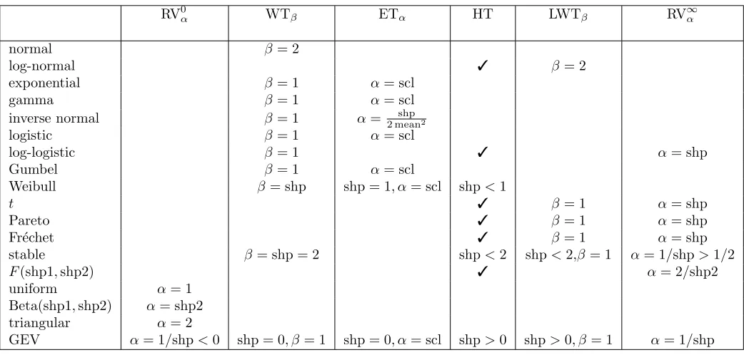
Table 1 summarizes the tail dependence for (X1, X2) using the norms from Examples2–4, under different tail

behaviors forR.

ν =Lp norm,p≥1 ν =L∞ norm ν =θmax +(1−θ) min,θ≥1

Radial variableR χX ηX χX ηX χX ηX

Regularly varying

FR∈RV∞−α,α >0 eq. (4) 1 eq. (4) 1 eq. (4) 1

Log-normal

−logFR(r)∼k(logr)2,k >0 0 1 0 1 2(θ−1)/(2θ−1) 1

Weibull-like

−logFR(r)∼krδ,k, δ >0 0 2−δ/p 0 1 2(θ−1)/(2θ−1) 1

a) exponential (δ= 1) 0 2−1/p 0 1 2(θ−1)/(2θ−1) 1 b) normal (δ= 2) 0 2−2/p 0 1 2(θ−1)/(2θ−1) 1 Log of exponential

−logFR(r)∼kexp(r),k >0 0 0 0 1 2(θ−1)/(2θ−1) 1

Exponential behavior atr?_<∞

FR(r?−1/r)∼kexp(−r),k >0 0 ND 0 1 2(θ−1)/(2θ−1) 1

Negative Weibull

FR(r?− ·)∈RV0α, α >0 0 ND 0 α/(1 +α) 2(θ−1)/(2θ−1) 1

a) uniform (r?_{= 1, α= 1) 0 ND 0 1/2 2(θ−1)/(2θ−1) 1}

Table 1: Values of χX and ηX for (X1, X2) = R(W1, W2) with different tail decay rates of the variable R and

angular variables defined onLp,L∞norms, and the norm of Example2. ND = not defined.

3

Unconstrained angular variables

We now treat the case where the support W is two-dimensional. As noted in Section 1, there are cases where (W1, W2) itself might have a random scale representation, and by redefining the scaling variable we get back to

the situation of one-dimensional W. We thus focus on constructions where this is not necessarily the case. To avoid additional complications we assume throughout this section that W1 and W2 share the common marginal

distributionFW. We also generally assume that the tail dependence coefficientχW and the residual tail dependence

coefficientηW of (W1, W2) exist, although some results may still be obtained with the latter undefined.

In Section 2, the constraints imposed by W being a unit sphere gave bounded marginal distributions forWj,

j = 1,2, and deterministic dependence between (W1, W2). For two-dimensional W, the variety of marginal and

dependence behaviors possible for (W1, W2) means that systematic characterization according only to the MDA of

R is more difficult. In fact, we need to consider different tail decays of both the radial variableR and the angular variableW since the combination of the two is crucial to classify the extremal dependence of (X1, X2) =R(W1, W2).

We focus on some interesting sub-classes that still incorporate a wide variety of structures and cover most of the parametric univariate distributions available forRandW.

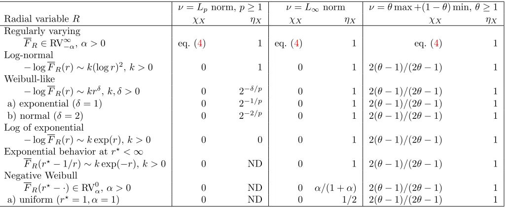
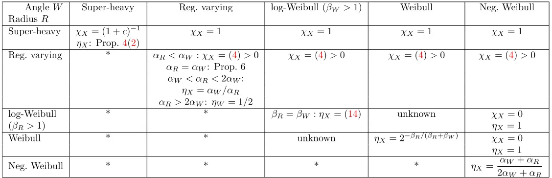
This section is structured according to the tail heaviness assumed for R, W, or both of them. In decreasing order we consider distributions with superheavy tails, regularly varying distributions, distributions of log-Weibull and Weibull type, and finally distributions with finite upper endpoint in the negative Weibull domain of attraction. Table2 summarizes the general results developed in the following, and Table 3 contains the extremal dependence coefficients for all combinations of tail decays of R andW for the specific, yet interesting example whereW1 and

W2 are independent.

3.1

Superheavy-tailed variables

Suppose that R or W is superheavy-tailed, i.e., logR or logW is heavy-tailed. This case naturally arises when considering random location constructions logR+ (logW1,logW2); we thus further assumeW >0 so that logWj,

RadiusR additional assumptions χX ηX

Superheavy tails

a) FW(x)/FR(x)→c Prop. 4 1+cχW_1+c 1

b)FR=o(FW) χW >0 χW 1

χW = 0,FR(x)≤CFW∧(x) 0 ηW χW = 0, FW∧=o(FR) 0 (2b)

RV∞_−α

R

a) E(WαR+ε_{)<∞ P(W >0) = 1 (4) 1}

b)FW ∈RV∞−αW

(i)αR> αW χW (12)

(ii)αR=αW Prop. 6 Prop. 6 1

LWTβR>1 FW, FW∧ ∈LWTβR χW (14)

WTβR FW ∈WTβW, FW∧∈WTβW∧ Prop. 8 Prop.8

Gumbel Prop.9(1) χW 1

Negative Weibull

Prop.9(2) χW ηW

Prop.9(3) 0 (17)

Table 2: Tail dependence summaries χX andηX for (X1, X2) =R(W1, W2) with different tail decay rates of the

radial variable R >0 and unconstrained variablesW1 d

=W2.

Proposition 4(Superheavy-tailed variables).

1. IfFlogR∈CE0 andFW(x)/FR(x)→c≥0asx→ ∞, thenηX= 1 and

χX= (1 +c χW)/(1 +c)>0. (11)

2. IfFlogW ∈CE0 andFR=o(FW), thenχX =χW. If further FlogR∈CE0 and

(a) FlogW∧∈CE0 with FR(x)/FW∧(x)≤C for a constantC >0 asx→ ∞, then ηX =ηW;

(b) FW∧ =o(FR), then, provided the limit exists,

ηX = lim

x→∞logFW(x)/logFR(x).

Example 5 (Independence model). In order to illustrate the results of this section, we consider the example where R, W1 and W2 are independent. In this case FW∧ = (FW)

2_{, χ}

W = 0 and ηW = 1/2. If FlogR ∈ CE0

and FW(x)/FR(x) → c ≥ 0 as x → ∞, then Proposition 4(1) yields asymptotic dependence in (X1, X2) with

χX = (1 +c)−1. Hence ifFlogR∈CE0 andW has a comparable tail, thenχX ∈(0,1), whilst ifW has tail lighter

than superheavy, thenχX = 1. On the other hand, ifW is superheavy-tailed withFlogW ∈CE0, then W∧ is also

superheavy-tailed. If R has lighter tail than W∧, then FR(x)≤CFW∧(x) for largex with some C > 0, and by

Proposition 4(2a) we haveχX= 0 and ηX = 1/2. The caseηX6=ηW may arise when the tail ofW dominates the

tail ofR and the tail ofR dominates the tail ofW∧. For a concrete example, consider log-Weibull tails inW and

R with FW(exp(x))∼exp(−xβ) and FR(exp(x))∼exp(−(1 +c)xβ), where 0< β, c <1. Then, ηX = (1 +c)−1

according to Proposition4(2b). The first row and column of Table3 summarize these results.

3.2

Regularly varying variables

In this section we consider the case whereR,W or both of them are regularly varying. WhenRis regularly varying with indexαR >0 and E(WαR+ε)<∞for someε >0, then the tail dependence coefficient χX is as described in

Proposition 1in Section 2.1. We firstly consider the case whereW is regularly varying with index αW >0 andR

is lighter tailed, i.e., either also regularly varying withαR > αW or even lighter tailed such as distributions in the

Gumbel or negative Weibull domain of attraction. Secondly, we study the case where bothRandW are regularly varying with the same indexαW =αR, which turns out to be particularly involved and which requires additional

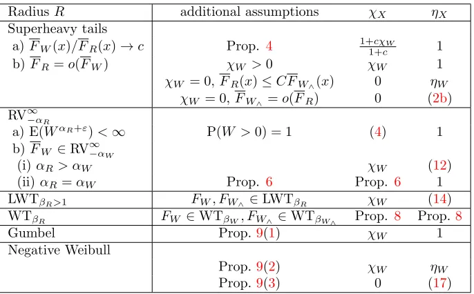
AngleW Super-heavy Reg. varying log-Weibull (βW >1) Weibull Neg. Weibull

RadiusR

Super-heavy χX= (1 +c)−1 χX= 1 χX = 1 χX= 1 χX = 1

ηX: Prop.4(2)

Reg. varying * αR< αW :χX= (4)>0 χX= (4)>0 χX = (4)>0 χX= (4)>0

αR=αW: Prop. 6

αW < αR<2αW:

ηX =αW/αR

αR>2αW: ηW = 1/2

log-Weibull * * βR=βW :ηX = (14) unknown χX = 0

(βR>1) ηX = 1

Weibull * * unknown ηX= 2−βR/(βR+βW) χX = 0

ηX = 1

Neg. Weibull * * * * ηX =

αW+αR

2αW +αR

Table 3: The values of χX and ηX for (X1, X2) =R(W1, W2) withW1, W2 d

=W independent, with different tail decay rates of the radial and angular variables. The *’s indicate that multiplication with R does not change the tail dependence of (W1, W2), i.e.,χX=χW = 0 andηX =ηW = 1/2. The combinations of Weibull and log-Weibull

tails remain open problems.

Proposition 5 (W regularly varying with R lighter). Let FW ∈ RV∞−αW, αW ≥ 0, and suppose that either

FR ∈ RV∞−αR with αR > αW, or R is in the Gumbel or negative Weibull domain of attraction; denote the latter

case by αR= +∞. Then χX =χW and

ηX=

(

αW/αR, ifαR< αW/ηW, ηW = 0or ηW not defined,

ηW, ifαR> αW/ηW or αR= +∞.

(12)

The case where R and W are regularly varying with the same indexα > 0 leads to various scenarios for the extremal dependence in (X1, X2). SinceFR, FW ∈RV−α∞ is equivalent toFlogR, FlogW ∈ETα, and ETα is closed

under convolutions, we have thatFlogX∈ETα (Watanabe, 2008, Lemma 2.5).

Proposition 6(Regularly varyingRandW with the same index). LetFR, FW ∈RV∞−αwithα >0. ThenηX= 1,

and we have the following:

1. IfFlogR∈CEα, and ifFW(x)/FR(x)→c≥0 asx→ ∞, then

χX =

E(Wα

∧) +c χWE(Rα)

E(Wα_{) +cE(R}α₎ .

2. IfFlogW ∈CEα andFR=o(FW), then χX=χW.

3. LetFlogR∈ETα,βR withβR≥ −1 and E(R

α_{) =∞if β}

R=−1, and letFlogW ∈ETα,βW.

(a) IfχW >0 and if eitherβW >−1 orβW =−1 and E(Wα) =∞, thenχX=χW.

(b) IfχW ≥0 and if eitherβW <−1 orβW =−1< βR and E(Wα)<∞, then χX=E(W∧α)/E(Wα).

(c) IfβR>−1,βW >−1 and E(W∧α+ε)<∞for someε >0, thenχX = 0.

Remark 4. Proposition 6 contains certain results of Proposition 4 as a special case when allowing for α = 0. Proposition6(1),(2) treats the case of convolution-equivalent tails in logRor logW, which are relatively light since the expectation E(Rα_{) or E(W}α_{) is finite; notice that ET}

α,β with β <−1 is an important subclass of CEα, see

Lemma 2.3 ofPakes(2004). The tail ofRis not dominated by that ofW in Proposition6(1), while it is dominated in Proposition6(2). Proposition6(3) shifts focus to relatively heavy tails inRwith E(Rα_{) =∞, such as the gamma}

Example 6(Independence model). We continue Example5, where nowW1andW2are independent and regularly

varying with indexαW, andRis regularly varying with indexαR. IfαR< αW, then we have asymptotic dependence

withχX given in (4). The same is true in general whenW has a lighter tail thanRthat is not necessarily regularly

varying. By Proposition5, if αW < αR <2αW, then (X1, X2) is asymptotically independent withηX =αW/αR,

and if αR > 2αW, then ηX = 1/2. In general, if R is even lighter tailed, it does not affect the coefficients χX

and ηX. IfαR =αW =α, then ηX = 1 and different scenarios for χX arise depending on the distributions ofR

and W: see Proposition 6. Suppose α > 0; since FW∧ ∈RV

∞

−2α, FX∧ ∼E(W

α

∧)FR, and so χX = E(W∧α)/c >0

if FX ∼cFR for some c >0. In particular, c = E(Wα) if FW ∈ETα,βW and FR ∈ETα,βR with βW < βR and

βW <−1. This fills the second row and column of Table3.

3.3

Log-Weibull-type variables

In this and the following section we concentrate on radial and angular variables in the Gumbel domain of attraction. Due to the large variety of distributions in this domain we consider subsets that include the most commonly used distribution families. We firstly study the case where bothRandW are log-Weibull-tailed; equivalently, logRand logW are Weibull-tailed. We recall that a random variableY is log-Weibull-tailed if

FY(y) =`(logy)(logy)γexp −α(logy)β

, `∈RV∞₀ , γ ∈_R, α, β >0, (13)

and we writeFY ∈LWTβ. The parameterβ has the predominant influence on the tail decay rate, withβ= 1 if and

only ifFY ∈RV∞−α, whileβ <1 gives superheavy-tailedFY, andβ >1 yields rapid variation ofY, i.e.,FY ∈RV∞−∞.

In the following, we denote theβ-parameters ofRandW byβRandβW, respectively. The superheavy-tailed case,

βR<1 orβW <1, is already covered by Section3.1, and the case of regularly varying tails withβR= 1 orβW = 1

is treated in Section3.2.

We therefore study the remaining case βR >1 and βW >1, which encompasses important distributions such

as the log-Gaussian. As in Section 3.1, it is more intuitive to consider the random location construction logR+ log(W1, W2), where we can apply convolution-based results. When independent heavy-tailed summands are involved

in the convolution, typically only one of the values of summands has a dominant contribution to a high values of the sum, resulting in relatively simple formulas; see Section3.1. On the contrary, in the light-tailed set-up all summands may contribute significantly when high values arise in the sum, rendering the tail analysis more intricate. Only relatively few general results on convolutions with tails lighter than exponential are available in the literature. The following lemma will be useful for this and the next section.

Lemma 1. Let (W1, W2) be a random vector with Wj ∼FW, j = 1,2, such that both FW ∈ WTβW and FW∧ ∈

WTβW∧, with other parameters also indexed byW andW∧.

1. IfβW∧=βW,αW∧ =αW, then, provided the limit exists,χW = limx→∞

`W∧(x)xγW∧

`W(x)xγW .

2. IfβW∧=βW, thenηW =αW/αW∧.

3. IfβW∧> βW, thenlogFW =o(logFW∧), andηW is not defined.

Remark 5. The proof of Lemma 1 is straightforward from (13). It also covers the case where W and W∧ are

log-Weibull-tailed, since the tail and residual tail dependence coefficients are invariant under monotonic marginal transformations.

We consider the set-up where the components R, W and W∧ are log-Weibull-tailed with the same coefficient

β > 1 and a simplified form of the slowly varying function ` by assuming that it is asymptotically constant, i.e.,

`(x)∼c >0.

Proposition 7 (Light-tailed random location withFR∈LWTβ,β >1). Suppose thatFR, FW, FW∧ ∈LWTβ with

possibly different parametersα, γ indexed by the correspondingR,W andW∧, but whereβ =βR=βW =βW∧ >1.

Assume that the slowly varying functions` behave asymptotically like positive constants.

1. IfχW >0, then χX=χW >0.

2. IfχW = 0, then χX= 0 and

ηX=ηW ×

α1/(β−1)_W ∧ +α

1/(β−1) R

α1/(β−1)_W +α1/(β−1)_R

!β−1

, (14)

Example 7 (Gaussian factor model). Suppose that logR is univariate standard Gaussian and that log(W1, W2)

is bivariate standard Gaussian, independent of R and with Gaussian correlation ρW ∈ (−1,1]. Then we have

log-Weibull tails with parametersβR=βW =βW∧ = 2,αR=αW = 1/2 andαW∧ = 1/(1 +ρW) (see Example 9).

Applying (14) givesηX=ηW ×(3 +ρW)/(2(1 +ρW)) = (3 +ρW)/4.

Example 8 (Independence model). As in Examples5 and 6 we let R, W1 andW2 be independent, and we now

assume that they are log-Weibull-tailed with equalβparameter. By independence,FW∧ ∈LWTβwithαW∧= 2αW.

Proposition7 givesχX= 0 with ηX calculated by formula (14).

3.4

Weibull-type variables

We now consider the case where R and W follow a Weibull-type distribution, a rich class in the Gumbel MDA. Recall that a variableY is of Weibull-type,FY ∈WTβ, if

FY(y) =`(y)yγexp −αyβ

, `∈RV∞₀ , γ∈R, α, β >0. (15)

Well-known examples of Weibull-tailed distributions are the Gaussian withβ = 2, the gamma withβ= 1 or, more generally, the Weibull whereβ is called the Weibull index.

For developing useful results, we further assume that, in addition toRandW,W∧also has a Weibull-type tail.

As previously, we index the corresponding` functions and the parameters α, γ in (15) by the variable name. We also recall Lemma1 concerning the dependence coefficients of the vector (W1, W2).

Proposition 8 (Weibull-type variables). Suppose that FR ∈WTβR,FW ∈WTβW andFW∧ ∈WTβW∧. We have

the following hierarchy of dependence structures:

1. If βW∧ = βW, αW∧ = αW, γW∧ = γW, then χX = χW = limx→∞`W∧(x)/`W(x), if the limit exists, and ηX=ηW = 1.

2. IfβW∧=βW,αW∧ =αW,γW∧< γW, then χX= 0 andηX =ηW = 1.

3. IfβW∧=βW,αW∧ > αW, thenχX = 0and

ηX =η

βR/(βR+βW)

W = (αW/αW∧)

βR/(βR+βW)

.

4. IfβW∧> βW, thenχX= 0 andηX =ηW = 0.

In all of the cases encompassed by Proposition8, (X1, X2) and (W1, W2) have the same tail dependence coefficient

χ, which can be positive only in case 1. In all other cases the variables are asymptotically independent, and only in case 3 the residual tail dependence coefficientη changes under the multiplication of the radial variableR. Since

βR/(βR+βW)∈(0,1), this always leads to an increase in dependence, that is,ηX > ηW.

Example 9 (Gaussian scale mixtures). To illustrate the most interesting case 3 in Proposition 8 we consider (W1, W2) following a bivariate Gaussian distribution with standardized margins and correlationρW. We have that

FW(x)∼rW(x) exp(−x2/2), FW∧(x)∼rW∧(x) exp{−x

2_{/(1 +ρ} W)},

where the tail distribution of the minimum follows from bounds on the multivariate Mills ratio (e.g.Hashorva and H¨usler, 2003), and rW and rW∧ are regularly varying functions. Therefore, ηW = (1 +ρW)/2 and Proposition8

confirmsHuser et al.(2017, Theorem 2) where

ηX=η

βR/(βR+2)

W ={(1 +ρW)/2}βR/(βR+2).

Example 10 (Independence model). We continue the example whereR, W1 and W2 are independent, and they

are now assumed to be Weibull-tailed. The variable W∧ is also Weibull-tailed with βW∧ =βW andαW∧ = 2αW.

Therefore, the third part of Proposition 8 entails that ηX = 2−βR/(βR+βW). This expression tends to 1/2 if

3.5

Variables in the negative Weibull domain of attraction

The remaining cases are those where R, W or both of them are in the negative Weibull MDA, with finite upper endpoint. Recall that a variableY is in the negative Weibull MDA if

FY(y?−s) =`(s)sα, `∈RV00, α >0. (16)

The case where R is superheavy-tailed or regularly varying and W satisfies (16) has been covered in part 1 of Proposition 4 and Proposition 1, respectively. On the other hand, the case where the tail of R satisfies (16) and

W is superheavy-tailed or regularly varying is treated by part 2 of Proposition4 and Proposition5, respectively. It remains to study the situation where one ofR or W is of form (16), and the other is in the Gumbel domain of attraction as defined in (8). In this section we focus on the case whereW∧has the same upper endpoint asW; for

a more detailed study whereW∧ can have a smaller upper endpoint, and W may have a point mass on its upper

endpoint, see Section2.

Proposition 9(Variables in the negative Weibull MDA). 1. Suppose thatRis in the Gumbel MDA with upper endpoint r? _{∈ (0,∞] and that W and W}

∧ satisfy (16) with parameters αW and αW∧, respectively. Then χX=χW andηX= 1.

2. Let R satisfy (16) and let W and W∧ be in the Gumbel MDA with equal upper endpoint w? ∈ (0,∞] and

auxiliary functionsbW andbW∧, such thatlimx→w?bW(x)/bW∧(x)exists. ThenχX =χW andηX =ηW.

3. Let R, W and W∧ all satisfy (16) with endpointsr?, w?, w? and parameters αR, αW and αW∧, respectively.

If αW∧ =αW thenχX =χW andηX = 1. IfαW∧ > αW thenχX=χW = 0 and

ηX = (αW +αR)/(αW∧+αR)> αW/αW∧ =ηW. (17)

Example 11 (Independence model). Continuing the running independence example, we now suppose thatFR, FW

satisfy (16) with parametersαR, αW. Clearly,FW∧ also satisfies (16), with parameterαW∧ = 2αW. The third part

of Proposition 9shows that

ηX= (αW+αR)/(2αW +αR)∈(1/2,1),

hence by varying the parametersαR, αW >0 we can attain the whole range of residual tail dependence coefficients

related to positive association.

4

Literature review and examples

Here we present an overview of related literature, detailing how existing examples and results fit into the framework of this paper.

Elliptical copulas Let Σ be a positive-definite covariance matrix with Cholesky decomposition Σ = AAT_,

and (U1, U2) be uniformly distributed on the L2 sphere {(w1, w2) : (w1, w2)T(w1, w2) = 1}. Then (X1, X2) =

RA(U1, U2)T has an elliptical distribution for anyR >0 called thegenerator. Therefore (W1, W2)T =A(U1, U2)T

lies on the Mahalanobis sphereW ={(w1, w2) : (w1, w2)TΣ−1(w1, w2) = 1}, and the extremal dependence in the

upper right orthant is unchanged by taking (Wj)+ = max(Wj,0). It is well known that (X1, X2) is asymptotically

dependent if and only ifR is in the Fr´echet MDA (Hult and Lindskog,2002, Theorem 4.3). In that case, the tail dependence coefficientχX is given by (4), withWj replaced by (Wj)+; see alsoOpitz(2013). ForRin the Gumbel

MDA, the scaling condition onν such thatτ(w)∈[0,1] yields Σ with diagonal elements 1, off-diagonal elements

ρ∈(−1,1), and residual tail dependence coefficient is given by Proposition2(1) withζ=τ(1/2) ={(1 +ρ)/2}1/2_.

Hashorva(2010) details calculation ofηX assumingRto be in the Gumbel MDA, providing an alternative

perspec-tive on the derivation. The spatial model ofHuser et al.(2017) is also covered by this case.

Example (Gaussian). The Gaussian distribution arises when FR(r) =e−r

2_/2

, so that by Corollary1,ηX=ζ2=

Archimedean and Liouville copulas Archimedean (respectively Liouville) copulas arise as the survival cop-ula when (W1, W2) is uniformly (respectively Dirichlet) distributed on the positive part of the L1 sphere W = {(w1, w2)∈[0,1]2:w1+w2= 1}, andR >0. That is, (X1, X2) =R(W1, W2) has aninverted Archimedean or

Li-ouville copula, whilst the Archimedean or LiLi-ouville copula itself is that of (t(X1), t(X2)), for a monotonic decreasing

transformationt. By takingt(x) = 1/x, we obtain 1/(X1, X2) = ( ˜X1,X˜2) = ˜R( ˜W1,W˜2), so Archimedean copulas

have a random scale representation with ( ˜W1,W˜2) constrained by functional dependence that is not represented by

a norm.

Archimedean copulas are typically defined in terms of a non-increasing continuous generator function ψ : [0,∞) → [0,1], such that C(u1, u2) = ψ(ψ−1(u1) +ψ−1(u2)). The link between ψ and the variable R ∼ FR is

given in equation (3.3) ofMcNeil and Neˇslehov´a(2009); ford= 2 this is

FR(r) =ψ(r)−rψ0(r+), r >0, (18)

whereψ0(r+) denotes the right-hand derivative ofψ.

Archimedean copulas are a special case of Liouville copulas, whose dependence properties are studied inBelzile and Neˇslehov´a (2018). For (X1, X2), their Theorem 1 states that R in the Fr´echet MDA leads to asymptotic

dependence, whilst the Gumbel and negative Weibull MDAs lead to asymptotic independence. The exponent func-tion given in their Theorem 1 matches equafunc-tion (6). In their Theorem 2, Belzile and Neˇslehov´a (2018) consider the extremal dependence properties of 1/(X1, X2) = ˜R( ˜W1,W˜2), i.e., the Liouville copula itself. Since the

recip-rocal of Dirichlet random variables have regularly varying tails, this links with Proposition 5 which states that asymptotic independence arises if ( ˜W1,W˜2) themselves are asymptotically independent and heavier-tailed thanR.

Proposition6(3c) is relevant if ˜Rand ˜W are regularly varying with the same index.

Example (Gumbel and inverted Gumbel copulas). The Gumbel, or logistic, Archimedean copula arises when

ψ(x) = e−xθ, θ ∈ (0,1]. By (18), FR(r) = e−r θ

(1 +θrθ_{)∈ WT}

θ. The copula of (X1, X2) is the asymptotically

independent inverted Gumbel copula (Ledford and Tawn, 1997). We haveζ=τ(1/2) = 1/2 and soηX = 2−θ by

Corollary1. The Gumbel copula is that of 1/(X1, X2) = ˜R( ˜W1,W˜2), withFR˜(r) =e−r

−θ

(1 +θr−θ), soFR˜∈RV ∞

−θ.

The dependence structure follows from Proposition 1 forθ <1 since E( ˜Wθ_{)<∞. Noting that ˜W}

∧ is a bounded

random variable,χX = 0 forθ= 1, as given by Proposition6(3c). In fact, forθ= 1, the copula is the independence

copula.

Archimax copulas Bivariate Archimax copulas were introduced by Cap´era`a et al. (2000) and extended to the multivariate case with a stochastic representation by Charpentier et al. (2014). They are so-called because of a connection to both Archimedean and extreme-value max-stable copulas. Letting ψ be the generator of an Archimedean copula, andV the exponent function defined in (5), a bivariate Archimax copula can be expressed as

C(u1, u2) =ψ◦V(1/ψ−1(u1),1/ψ−1(u2)), such that takingV(x1, x2) = 1/x2+ 1/x2 — corresponding to the

inde-pendence max-stable copula — yields an Archimedean copula, whilst takingψ(x) =e−xyields a max-stable copula.

Charpentier et al.(2014) show that the vector (X1, X2) =R(W1, W2) has an inverted Archimax copula ifFR is as

in (18), and P(W1≥w1, W2≥w2) = max(0,1−V(1/w1,1/w2)). Hence ( ˜X1,X˜2) = 1/(X1, X2) = ˜R( ˜W1,W˜2) has an

Archimax copula. We haveF_W˜(w)∈RV∞−1andχ_W˜ = 2−V(1,1) which is positive unlessV(x1, x2) = 1/x2+ 1/x2.

If ˜R has a lighter tail then Proposition 5 gives χ_X˜ = χ_W˜, whilst if ˜R is the same or heavier, the results of

Propositions 1, 4 or 6 are relevant. The inverted case follows similarly to the calculations in Section2 since the margins of W1, W2 are uniform and the zero-truncation in the copula for (W1, W2) means that there is mass on {w∈[0,1] :V(1/w,1/(1−w)) = 1} wheneverV(1/w1,1/w2)>1, whereV(1/x1,1/x2) defines a norm.

Example (Gumbel Archimax). Taking V(x1, x2) = (x −1/θ

1 +x

−1/θ 2 )

θ_{, the exponent function of the logistic, then}

the corresponding Archimax copula is C(u1, u2) = ψ{(ψ−1(u1)1/θ +ψ−1(u2)1/θ)θ}, which is Archimedean with

generator ψ(xθ_{) (Charpentier et al., 2014). If ψ(x) = e}−xα

, α ∈ (0,1], then we obtain the Gumbel copula with parameterθα. Tail dependence results can then be obtained as in the example above, or considering the Archimax structure. Following the latter, for ˜X Proposition 1 gives χ_X˜ = 2−V(1,1)α = 2−2θα, for α ∈ (0,1) whilst

Proposition 6(3a) gives the extension to α= 1. For the inverted copula ηX = (2−θ)α, following similar lines to

Proposition2.

Multivariate (ρ-)Pareto copulas Letρ: (0,∞)2 →(0,∞) be a positive homogeneous function. Multivariate

ρ-Pareto copulas arise whenFR(r) =r−1, i.e. standard Pareto, and the random vector (W1, W2) is concentrated

on W = {(w1, w2) ∈ R2+ : ρ(w1, w2) = 1} with marginals satisfying E(W) < ∞ (Dombry and Ribatet, 2015).

Pareto distributions (Rootz´en and Tajvidi,2006; Ferreira and de Haan,2014;Rootz´en et al.,2018). Such copulas are asymptotically dependent, except for the case outlined in Section2.1, withχX given by (4). Although we have

focused on norms andρneed not be convex, there is nothing in Proposition1requiring this.

Example (Bivariate Pareto copula associated to the Gumbel copula). Since the Gumbel copula is a max-stable distribution, it has an associated Pareto copula. IfZ has densityfZ(z) =h(z) max(z,1−z)21−θ, wherehis given

by (7), then (X1, X2) =R(W1, W2) =R(Z,1−Z)/max(Z,1−Z) withFR(r) =r−1leads to the associated bivariate

Pareto copula. The distribution function of (X1, X2) is

P(X1≤x1, X2≤x2) ={V(min(x1,1),min(x2,1))−V(x1, x2)}/V(1,1),

whereV(x1, x2) = (x−1/θ1 +x −1/θ

2 )θ is the exponent function for the Gumbel distribution.

Model of de Haan and Zhou (2011) They describe the losses of two banks by a factor modelSj =C+Lj,

j= 1,2, whereFLj ∈RV ∞

−αandFC∈RV∞−β. Forβ < αthey show thatS= (S1, S2) is completely asymptotically

dependent, i.e.,χS = 1, and forβ =αthey obtainχS ∈(0,1). Ifα < β <2αasymptotic independence arises with

ηS =α/β, and ifβ >2αthenηS= 1/2. Our proposition4yields the same results as special cases withR= exp(C)

andWj = exp(Lj),j = 1,2.

Model of Wadsworth et al.(2017) They consider the copula induced by takingR to be generalized Pareto,

FR(r) = (1 +λr)−1/λ+ , and W={(w1, w2)∈[0,1]2:k(w1, w2)k∗= 1} wherek · k∗ is a symmetric norm subject to

certain restrictions. These restrictions mean that λ≤0 corresponds to asymptotic independence; the residual tail dependence coefficientηX is as given in Proposition2forλ= 0 withζ=τ(1/2) =k(1,1)k−1∗ , and Proposition3for

λ <0. We note that if the normν has certain shapes that were excluded inWadsworth et al. (2017), asymptotic dependence is possible forλ≤0. WhenR is in the Fr´echet MDA (λ >0) then asymptotic dependence holds with

χX given by (4).

Model of Krupskii et al. (2016) They consider location mixtures of Gaussian distributions, corresponding to scale mixtures of log-Gaussian distributions. According to their Proposition 1, asymptotic dependence occurs when the location variable is of exponential type, i.e. the scale is of Pareto type; the givenχXcan then be obtained via (4).

When the location is Weibull-tailed but with shape in (0,1), the scale is superheavy-tailed, withFR∈RV∞0 , and

perfect extremal dependence (χX = 1) arises, as noted in Remark 3 following Proposition 1. When the random

location is Weibull-tailed with shape in (1,∞) then the random scale R is in the Gumbel MDA and asymptotic independence arises. If FlogR ∈ WT2 has the same Weibull coefficient 2 as the standard Gaussian logW and as

logW∧ (provided that ρ= cor(log W1,log W2)∈(−1,1]), then we can apply Proposition7 to calculate the value

ofηX given as

ηX=ηW

αW∧+αR αW +αR

=1 +ρ 2

(1 +ρ)−1+αR

1/2 +αR

= 1 + (1 +ρ)αR 1 + 2αR

,

which extends the results ofKrupskii et al.(2016). Specifically, with standard Gaussian logRwe getηX= (3+ρ)/4,

see Example7.

Model ofHuser and Wadsworth(2018) They consider scale mixtures of asymptotically independent vectors where both R andW have Pareto margins with different shape parameters. Asymptotic dependence arises when

R is heavier tailed; χX is then given by (4), whilst asymptotic independence arises when W is heavier tailed and

ηX is given by (12). When R and W have the same shape parameter, their assumption ηW < 1 implies that

E(W∧α+ε)<∞for some ε >0, giving asymptotic independence by Proposition6(3c).

Various other articles also focus on polar or scale-mixture representations. Hashorva (2012) examines the extremal behavior of scale mixtures when R is in the Gumbel MDA. He considers both one- and two-dimensional W, both with similarities and differences to our set-up. For one-dimensionalW, he assumes a functional constraint of the form (W1, W2) = (W, ρW +z∗(W)) for measurable z∗ : [0,1]→(0,∞); ρ ∈(−1,1) (the specification also

allows for negative components, but we focus here on the positive part). Constraints to certain norm spheres, such as the Mahalanobis orLp norm, could be written in this way, however examples such as the L∞ norm could

Hashorva(2012), we typically assume symmetry, there are nonetheless some connections between the results in our Section3.5and that paper.

Nolde(2014) provides an interpretation of extremal dependence in terms of agauge function (see alsoBalkema and Nolde (2010) andBalkema and Embrechts (2007)), which, loosely speaking, corresponds to level sets of the density in light-tailed margins. The main result ofNolde(2014) (Theorem 2.1) is presented in terms of Weibull-type margins, such that−logFX ∈RV∞δ ,δ >0; in terms of Section2, this corresponds to−logFR∈RV∞δ . By noting

that where the density ofR, fR, exists, the joint density of (X1, X2) =R(τ(Z), τ(1−Z)) is

f(X1,X2)(x1, x2) =fR(ν(x1, x2))fZ(x1/(x1+x2))ν(x1, x2)/(x1+x2) 2_,

the gauge function of (X1, X2) is obtained asν when −logFR ∈RV∞δ , using Proposition 3.1 therein. We found

ηX =ζδ, withζ=ν(1,1)−1, precisely as inNolde(2014).

Various papers focus on extremal dependence arising from certain types of polar representation, but from a conditional extremes perspective (Heffernan and Tawn, 2004; Heffernan and Resnick, 2007). This is different to our focus; here we examine the extremal dependence as both variables grow at the same rate. In the conditional approach, different rates of growth may be required in the different components. Abdous et al. (2005) examine conditional limits in the context of elliptical copulas, whilstFoug`eres and Soulier(2010) andSeifert(2014) consider the constrainedW case, withR in the Gumbel MDA.

5

New examples

We present two new constructions that have the desirable property of smoothly interpolating between asymptotic dependence and asymptotic independence, whilst yielding non-trivial structures within each class. By smoothness, we mean that the transition between classes occurs at an interior point,θ0, of the parameter space Θ, and, assuming

increasing dependence with θ, limθ→θ0+χX = 0, limθ→θ0−ηX = 1. To our knowledge, the only other models in

the literature with this behavior are (i) that of Wadsworth et al.(2017), whereν(x, y) = max(x, y) and FR(x) =

(1 +λx)−1/λ₊ , λ ∈ R, and (ii) that of Huser and Wadsworth(2018) where FR(x) = x−1/δ, FW(x) = x−1/(1−δ),

δ∈(0,1), andηW <1. The first example is constructed using constrained (W1, W2) (Section2), where the required

ingredients areFR,ν, andFZ, whilst the second uses unconstrained (W1, W2) (Section3) with ingredientsFR,FW

and the dependence structure of (W1, W2).

5.1

Model 1

In Propositions2 and 3, it was demonstrated how the shape of ν affects the tail dependence of (X1, X2) whenR

is in the Gumbel or negative Weibull MDA. In Example2, a particular norm that yields asymptotic dependence was given; here we extend the parameterization of this norm and use our results to present a new asymptotically (in)dependent copula. Since the cases whereR has finite upper endpoint r? _{<∞lead to undefined η}

X, we focus

onr?=∞.

Proposition 10. Let R be in the Gumbel MDA with r? _{=∞ and let ν(x, y) = θmax(x, y) + (1−θ) min(x, y),}

θ≥1/2. Then for(W1, W2)defined through (10)andZ satisfying the conditions in Section2.2,

χX = max(2(θ−1)/(2θ−1),0) ηX= lim

x→∞logFR(x)/logFR(x/min(θ,1)).

We note that if−logFR∈RVδ, for example, then we have a continuous parametric family exhibiting asymptotic

dependence forθ >1 withχX = 2(θ−1)/(2θ−1), and asymptotic independence forθ≤1 withηX =θδ. To make

things concrete, we propose the following model.

Model 1.

FR(r) =e−r δ

ν(x, y) =θmax(x, y) + (1−θ) min(x, y), θ≥1/2 Z ∼Beta(α, α).

The set of models defined in Proposition 10, exemplified by Model 1, has some rather interesting behavior in the extremes. Whilst the limiting quantities χX, ηX are given in Proposition 10, the subasymptotic behavior

of (X1, X2), in particular the behavior of the slowly varying function ` in (2), is not prescribed by any of the

propositions in this paper. Combining equations (2) and (3), define

χX(q) = Pr(X1≥FX−11(q), X1≥F −1

so that for ηX = 1, χX(q) = `(1−q). For Model 1 we find that χX(q) is not necessarily monotonic, and may

decrease before increasing to a positive limit value. Figure 2 shows χX(q) for various parameterizations of the

model. This non-monotonic behavior appears uncommon; to our knowledge there are no well-known theoretical examples of this.

1−q

χX

(

q

)

10−1 ₁₀−2 ₁₀−3 ₁₀−4 ₁₀−5 ₁₀−6 ₁₀−7

0.0

0.1

0.2

0.3

0.4

θ =0.75 , α =1

δ =0.5

δ =1

δ =1.5

δ =2

δ =3

1−q

χX

(

q

)

10−1 ₁₀−2 ₁₀−3 ₁₀−4 ₁₀−5 ₁₀−6 ₁₀−7

0.0 0.1 0.2 0.3 0.4 0.5

θ =1 , α =1

1−q

χX

(

q

)

10−1 ₁₀−2 ₁₀−3 ₁₀−4 ₁₀−5 ₁₀−6 ₁₀−7

0.0 0.1 0.2 0.3 0.4 0.5

θ =1.25 , α =1

1−q

χX

(

q

)

10−1 ₁₀−2 ₁₀−3 ₁₀−4 ₁₀−5 ₁₀−6 ₁₀−7

0.0

0.1

0.2

0.3

0.4

θ =0.75 , δ =1

α =0.5

α =1

α =1.5

α =2

α =3

1−q

χX

(

q

)

10−1 ₁₀−2 ₁₀−3 ₁₀−4 ₁₀−5 ₁₀−6 ₁₀−7

0.0 0.1 0.2 0.3 0.4 0.5

θ =1 , δ =1

1−q

χX

(

q

)

10−1 ₁₀−2 ₁₀−3 ₁₀−4 ₁₀−5 ₁₀−6 ₁₀−7

0.0 0.1 0.2 0.3 0.4 0.5

θ =1.25 , δ =1

Figure 2: Theoretical χX(q) for Model1 plotted against 1−qon a logarithmic scale for q∈[1−10−1,1−10−7].

Different columns show different values ofθ; thick horizontal lines show the true limiting values ofχX = (0,0,1/3)

(left-right). Top row: δvaries within a panel; bottom row: αvaries within a panel.

5.2

Model 2

The following proposition collates results from Propositions1and9, and provides a general principle for constructing new dependence models permitting both asymptotic dependence and asymptotic independence.

Proposition 11. Let R be in the MDA of a generalized extreme value distribution with shape parameter ξ ∈ _R, and let (W1, W2)with W1

d

=W2 d

=W have χW = 0, well-definedηW ∈(0,1), andFW(w?− ·)∈RV0αW,αW >0.

Then

1. Forξ >0,χX =E(W 1/ξ

∧ )/E(W1/ξ),ηX = 1,

2. Forξ= 0,χX = 0,ηX = 1,

3. Forξ <0,χX = 0,ηX = (1−ξαW)/(1−ξαW/ηW).

The model construction opportunities from Proposition11are quite varied; specifically takingFRthat permits

all three tail behaviors produces a flexible range of models spanning the two dependence classes. We therefore propose the following concrete model, based on our running independence example.

Model 2.

For the special case α = 1, i.e, W ∼ Unif(0,1), one can explicitly calculate χX and VX as well as ηX. By

Proposition11, forξ <0,ηX = (1−ξ)/(1−2ξ) with limξ→0−ηX = 1, andχX = 0; forξ= 0,χX = 0,ηX = 1, and

forξ >0,χX = 2ξ/(2ξ+ 1), whilst

VX(x1, x2) = min(x1, x2)−1+

1 2ξ+ 1

_min(x

1, x2)

max(x1, x2)

ξ

max(x1, x2)−1. (19)

The limits of (19) as ξ → 0 and ξ → ∞ are x−1₁ +x−1₂ and min(x1, x2)−1, corresponding to independence and

perfect dependence (e.g. Beirlant et al., 2004, Ch. 8). Figure3 displays the function χX(q) for Model 2 across a

range of differentαandξ values.

1−q

χX

(

q

)

10−1 ₁₀−2 ₁₀−3 ₁₀−4 ₁₀−5 ₁₀−6 ₁₀−7

0.0

0.1

0.2

0.3

0.4

0.5

0.6

0.7

α =0.5

ξ =0.2

ξ =0.1

ξ =0

ξ = −0.1

ξ = −0.2

1−q

χX

(

q

)

10−1 ₁₀−2 ₁₀−3 ₁₀−4 ₁₀−5 ₁₀−6 ₁₀−7

0.0

0.1

0.2

0.3

0.4

0.5

0.6

0.7

α =1

1−q

χX

(

q

)

10−1 ₁₀−2 ₁₀−3 ₁₀−4 ₁₀−5 ₁₀−6 ₁₀−7

0.0

0.1

0.2

0.3

0.4

0.5

0.6

0.7

α =2

Figure 3: Theoretical χX(q) for Model2 plotted against 1−qon a logarithmic scale for q∈[1−10−1,1−10−7].

Different columns show different values of α; dashed horizontal lines show the true limiting values ofχX, which

depends onξ(and is zero forξ≤0).

6

Discussion

The paper studies the extremal properties of copulas (X1, X2) =R(W1, W2) and determines the tail and residual

tail dependence coefficientsχX andηX, respectively.

In Section2, where (W1, W2) is constrained to the sphere of some norm, classical results on multivariate Pareto

copulas are recovered for regularly varying R, whereas new structures are obtained for distributions of R with light tails or finite upper endpoint. In particular, for the Gumbel MDA we get a large variety of behaviors for asymptotically independent (X1, X2) that strongly depend on the auxiliary function b ofR and the shape of the

ν-sphere. This extends the results of Wadsworth et al.(2017) who considered only the exponential distribution in this class.

For unconstrained distributions of bothRandW, Section3formalizes the general intuition that heavier tails of

Rintroduce more additional dependence in (X1, X2). The results summarized in Table3for the special case of the

independence model allow for several conclusions. The most interesting (and involved) situations figure along the main diagonal whereR andW have similar tail behavior. Above this main diagonal,R is so heavy that it mostly dominates the extremal dependence in (X1, X2). On the other hand, below the diagonal, R is too light tailed,

relatively toW, to have an impact on the tail dependence coefficients χX andηX. Similar observations hold true

for the more general case of arbitrary dependence in (W1, W2) summarized in Table 2.

We note that there is a clear overlap between the results obtained in Sections2 and3. If one considersχW as

derived from the shape of W, then many results in Section 2 are obtained from Section3, just as Proposition1

is relevant in both sections. However, the separate treatment seems justified on the grounds of the importance of such constructions, and the additional insight gained in focusing on the shape ofW.

Multivariate analogs of the upper and residual tail dependence coefficients are obtained by considering the d -variate survival function P(X1≥x1, . . . , Xd≥xd) in (2) and (3). For random scale constructions inddimensions,

the results from Section 3 are all directly applicable if theWj components have common margins, since similarly

to the bivariate case, we only need to consider the two variables X∧ = Rmin(W1, . . . , Wd) and Xj =RWj. An

The above results provide a general and unifying framework to analyze bivariate extremal dependence, and Section4shows that they cover many of the existing examples in the copula and the extreme value literature. Most importantly, combining the insights from different sections enables the construction of numerous new statistical models that smoothly interpolate between asymptotic dependence and independence; see Section5for two instances. Although our focus was on dependence, knowledge on how the marginal scales ofRandW and the dependence properties of (W1, W2) influence the dependence of (X1, X2) makes it easier to construct models (X1, X2) that

naturally accommodate both marginal distributions and dependence of multivariate data. Such modeling avoids what may be construed as the artificial separation of modeling of margins and dependence known as copula modeling. For example, in factor constructions based on independent random variables, such as the ones with independentW1

andW2discussed throughout, our results give guidance on the relative tail heaviness ofRwith respect to (W1, W2)

necessary to transition from asymptotic independence to asymptotic dependence in (X1, X2), and both heavy- or

light-tailed marginal distributions are possible by considering the distribution of either (X1, X2) or log(X1, X2) as

a model for data.

In Sections 2 and 3, we often considered the simplification W1 d

= W2, yielding X1 d

= X2, which allows the

coefficients χX and ηX to be calculated without reference to marginal quantile functions. A weaker sufficient

condition for this isFX1(x)∼FX2(x) asx→x

?_{, withx}?_{a common upper end point. To see this sufficiency, define}

xq= min{FX−11(q), F −1 X2(q)},x

q _{= max{F}−1 X1(q), F

−1

X2(q)}, and note that

P(X1≥xq, X2≥xq)

max{FX1(x q_{), F}

X2(x q_)} ≤

P(X1≥FX−11(q), X2≥F −1 X2(q))

1−q ≤

P(X1≥xq, X2≥xq)

min{FX1(xq), FX2(xq)}

, (20)

where max{FX1(x q_{), F}

X2(x

q_{)} = min{F}

X1(xq), FX2(xq)} = 1−q. Consequently, the tail dependence coefficient

χX of (X1, X2), if it exists, is bounded between the limit superior of the left-hand side and the limit inferior of

the right-hand side in (20), respectively, for q → 1. Whilst these bounds hold in general for common upper end point, they deliver the precise coefficient χX only if FX1(x) ∼FX2(x), x→ x

? _{or both limits are zero. Similar}

arguments apply to the residual tail dependence coefficient ηX, where the corresponding bounds determine ηX

under the weaker requirement logFX1(x)∼logFX2(x),x→x ?_.

Whilst our focus has been on the coefficients χX and ηX, we note that there are important aspects of the

dependence structure that are not described by these coefficients. For example, in Section2, we found that when

Rwas in the Gumbel or negative Weibull MDA,χX andηX depended only on the shape ofν and the distribution

ofR, but not at all on the distribution ofZ. Nonetheless, the latter plays an important role in the behavior of the slowly varying function`in (3), which was exemplified in Figure2.

7

Proofs

This section contains proofs of propositions from Sections 2, 3 and 5. Proofs of lemmas are deferred to Ap-pendix A. Recall that in the case of common marginal distributions FX with upper endpoint x?, the tail

de-pendence coefficient is χX = limx→x?F_X∧(x)/F_X(x), whilst the residual tail dependence coefficient is η_X =

limx→x?logF_X(x)/logF_X∧(x).

7.1

Proofs for Section

2

Proof of Proposition1. Since E(W_jα+ε) < ∞, j = 1,2, Breiman’s lemma (Breiman, 1965, see also Lemma 8 in AppendixA) gives

FXj(x)∼E(W α

j )FR(x), x→ ∞, (21)

so thatFXj ∈RV ∞

−α. Now consider the quantile functions ofXj andR; denote these by F_Xj−1(q), F_R−1(q). Suppose

firstly thatα >0. Taking the reciprocal of relation (21), and using Proposition 2.6 (vi) ofResnick(2007), we have

F_X−1

j(q)∼F −1 R (q)E(W

α j)

1/α_{, q→1. (22)}

Consider now

P(X1≥FX−11(q), X2≥F −1

X2(q)) = P

Rmin

_W

1

E(Wα 1)1/α

[1 +o(1)], W2

E(Wα 2)1/α

[1 +o(1)]

≥F_R−1(q)