© 2019, IRJET | Impact Factor value: 7.34 | ISO 9001:2008 Certified Journal
| Page 838
Freight and Margin Optimisation in Building Material Industry using
Data Analytics and Network Optimisation Technique (Case Study:
Indian Ceramic Product Manufacturing Company)
Sanjeeva
1, Akash Kumar
21
S.P. Jain Institute of Management and Research, Mumbai, Maharashtra, India,
Indian Institute of Technology (ISM) Dhanbad, Jharkhand, India.
2
Indian Institute of Technology (ISM) Dhanbad, Jharkhand, India.
---***---Abstract -
This case study aims at understanding the causeof spiraling freight cost and dwindling margin of a building material company in a country in South Asia. In this study, sales data, transportation data and margin variation in different geographies of the country were analyzed and optimisation of freight and profit margin were done using the concept of network optimization tool and data analytics tools like Solver. The results of analysis throw pleasant surprises in the form of potential improvements above 30%.
Key Words: Average Radial Distance, Freight Index, Freight Optimisation, Margin Optimisation
1. INTRODUCTION
Optimization means maximizing the return at a given risk level or risk is minimized for a given expected return [1]. According to the great management consultant Peter Drucker, “Knowledge has to be improved, challenged and increased constantly, or it vanishes.” In reference to a supply chain, without constant study, a company can lose sight of how its supply chain impacts the entire business [2]. This case study is about a building material company in a country in South Asia which has 6 number of manufacturing locations across the country and 26 number of sales hubs. Before the study, the scenario was as follows. The average radial distance over which the finished goods were being transported was 768 miles and the freight index of the company was 3.10 cents/ton/mile. Total weight of material transported from all manufacturing locations in a month was 36 thousand tons on average. The total average freight for the transportation of the finished goods in a month was approximately USD 900,000. Also, the total operating margin of the company was stagnating at USD 5 million per month for last couple of years. We analysed the data to calculate average radial distance and freight index for each manufacturing location. We found that these indices varied from one manufacturing location to another. Further, we tried to analyse the relationship between average radial distance and freight index. Whereas, overall, a good degree of correlation was shown, some manufacturing locations didn’t conform to the relationship. Considering the fact that each manufacturing location demonstrated its own pattern of SCM cost, we inferred that SCM networks of all or at least
some manufacturing locations were not optimised. Considering this and also the fact that freight bill was considerably high, we decided to carry out network optimisation.
1.1 Aims & Objective
This study was carried out with following objectives:
To optimize the cost of transportation of finished goods.
To maximise the profit of the company by analysing the contribution (Price realised – variable cost) variation in different geographies of the country and optimising the same.
2. METHODOLOGY
Following concepts and approach were used in this study
2.1 Concept of Average Radial Distance and Freight Index
Average Radial Distance is the weighted average distance (by weight) from a manufacturing location over which the finished products are being transported. This index gives us an indication about how well the manufacturing location is located with respect to the market.
Freight Index is defined as cents spent to transport 1 ton of finished products over 1 mile.
We calculated this index for all the manufacturing locations. This index provides an indication about freight cost efficiency of each manufacturing location.
© 2019, IRJET | Impact Factor value: 7.34 | ISO 9001:2008 Certified Journal
| Page 839
Calculation Framework:
For a particular manufacturing location:
Let total quantity dispatched per month to each sales hub from that manufacturing location be T1, T2, T3…….,TN
Let Distance of each sales hub from that manufacturing location be D1, D2, D3…….,DN.
Let Freight per ton from the manufacturing location to each sales hub be F1, F2, F3…….,FN.
Total tonnage = Σ Ti
Total freight = Σ Fi Ti
Total Ton-miles = Σ Ti Di
Total freight /miles = Σ (Fi Ti / Di)
Freight Index for the manufacturing location (F.I.) = (Total freight /miles) / Total tonnage = [Σ (Fi Ti / Di)] / [Σ Ti]
Average Radial Distance = Total Ton-miles / Total tonnage = [Σ Ti Di] / [Σ Ti]
Using above concept, Freight Index and Average Radial Distance of all the manufacturing locations were calculated.
Having calculated the above parameters for individual manufacturing locations, the Freight Index of the Company was calculated which came out to be 3.10 cents/ton/mile. Average Radial Distance before optimisation was 768 miles. As a result of Network Optimisation, the Average Radial Distance came down to 529miles. This in turn lead to significant freight saving.
It may apparently seem that a manufacturing location with lower Average Radial Distance would have lower average freight. But, through our study, we busted this myth and brought a different perspective through the concept of Freight Index (FI). Freight Index looks at freight with respect to not only per unit weight moved, but also per unit distance moved.
Relation between Average radial distance and Freight Index of individual manufacturing location:
Manufacturing locations Freight Index
(cents/ton/mile) Average Radial Distance (miles)
RAK04 3.34 362
NUK03 3.61 429
WED02 3.45 588
JIV06 3.11 691
NEP01 2.99 839
JAR05 2.97 1023
Correlation Coefficient between FI and Average
Radial Distance -0.84
From above table and graph, it can be very well seen that there is a very high degree of negative correlation between average distance moved and Freight Index. This explains, to a great extent, why Freight Index of JAR05, NEP01 and JIV06 are low and that of NUK03, RAK04 and WED02 are high. Manufacturing location with longer average radial distance have lower freight per ton per mile. This is so because a vehicle is better utilized if it moves continuously for longer period of time before every stoppage for loading/unloading.
At the same time, we also realised that the Freight Index of WED02 and NUK03 are higher than that predicted by the regression formula. This shows that apart from distance, there are other reasons which are jacking Freight Index of WED02 and NUK03. Some of these reasons have to do with terrain, local labour situation and so on. For example, geographies with different terrain tend to have higher F.I. Geographies with high labour cost also tend to have higher F.I.
Further, a considerably high value of R- square in the above graph shows high degree of predictability of this equation.
Thus, freight equation developed during this study started being used to benchmark and develop clean sheet costing for use during freight negotiation.
2.2 Concept of Network Optimisation for optimisation of Freight and Margin
Freight Optimisation:
First of all, sales data i.e. dispatched quantities from each manufacturing location to each sales hub were collected and then the data were organised in the following format:
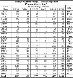
Tonnage matrix: This matrix contains the total dispatched quantities in tons from each manufacturing location to respective sales hub (Table 1).
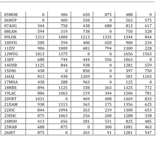
Distance Matrix: This matrix contains the distance of each manufacturing location from respective sales hub (Table 2).
© 2019, IRJET | Impact Factor value: 7.34 | ISO 9001:2008 Certified Journal
| Page 840
I. Production capacity of each manufacturing location was considered constant i.e. total dispatched quantity from a particular manufacturing location was considered constant.
II. Total demand of each sales hub was considered constant.
Considering all these factors, the analytical tool called ‘Solver’, calculates optimal scenario showing which manufacturing location should serve which market to minimise the total freight for the company.
Although, this analysis has been done at product category level, for the sake of simplicity, we are producing analysis result for all the products taken together.
[image:3.595.304.564.80.318.2]The optimised tonnage matrix is shown in Table 3.
Table 1
As – Is Scenario (For freight optimisation study)
Tonnage Matrix showing As - Is dispatch pattern (Average Monthly ‘tons’)
Sales Hubs
Manufacturing locations
Total
NEP01 WED02 NUK03 RAK04 JAR05 JIV06
01LED 309 171 9 0 743 51 1282
02CUL 118 47 21 0 791 214 1192
03AHG 25 73 51 0 541 32 722
04AHC 388 158 43 9 1467 185 2250
05MOB 0 288 190 52 611 0 1141
06NUP 0 79 153 0 608 184 1024
07AOG 321 1 80 16 97 49 564
08GAN 45 8 29 0 20 25 127
09LOK 295 98 93 16 913 932 2348
10DYH 401 55 322 121 492 79 1470
11ZIV 69 68 43 52 174 491 897
12WUG 18 16 0 82 120 236
13JIV 56 31 96 121 140 0 445
14UHB 57 25 22 0 181 161 445
15DNI 211 0 95 0 1012 251 1569
16IAJ 146 147 142 0 784 107 1326
17MHA 336 149 56 0 734 0 1275
18NRE 846 16 286 439 1456 624 3668
19LAC 418 41 146 182 351 1113 2252
20VRT 282 0 197 5 462 558 1504
21DAM 370 78 219 233 399 365 1664
22IOC 267 9 73 311 484 548 1693
23EHC 958 48 188 332 698 1248 3473
24BUH 152 15 168 33 182 49 598
25NAB 345 45 0 230 567 517 1703
26IRT 160 0 132 214 468 579 1552
Total 6591 1668 2855 2366 14457 8484
Table 2
Distance Matrix (For freight optimisation study)
Distance Matrix (Miles)
Sales
Hubs NEP01 WED02 Manufacturing locations NUK03 RAK04 JAR05 JIV06
01LED 956 500 1313 0 719 1175
02CUL 925 519 1238 0 1063 1081
03AHG 963 531 1313 0 728 1175
04AHC 1100 719 1500 1738 863 1331
05MOB 0 406 650 875 488 0
06NUP 0 400 550 0 563 575
07AOG 344 750 438 688 813 617
08GAN 594 319 738 0 750 528
09LOK 1313 1000 1213 1335 1344 844
10DYH 500 594 400 650 900 234
11ZIV 906 1000 681 794 1300 228
12WUG 1813 1375 0 0 1656 1563
13JIV 688 744 444 556 1063 0
14UHB 1125 844 938 0 1281 559
15DNI 438 0 850 0 397 750
16IAJ 813 438 1269 0 581 1163
17MHA 438 288 963 0 125 0
18NRE 894 1125 338 363 1325 772
19LAC 806 1063 219 344 1206 781
20VRT 1031 0 469 408 1469 833
21DAM 938 1313 363 175 1356 625
22IOC 844 1094 263 219 1300 653
23EHC 875 1063 256 200 1288 338
24BUH 413 656 281 531 825 485
25NAB 688 875 0 300 1081 463
26IRT 875 0 263 91 1281 547
Table 3
Optimised Scenario (For freight optimisation study)
Tonnage Matrix showing optimum dispatch pattern considering same production capacity of each manufacturing location and same demand of
each sale hub (Average Monthly ‘tons’)
Sales Hub
Manufacturing locations
Total
NEP01 WED02 NUK03 RAK04 JAR05 JIV06
01LED 0 0 0 0 1282 0 1282
02CUL 0 0 0 485 707 0 1192
03AHG 0 0 0 0 722 0 722
04AHC 0 0 0 0 2250 0 2250
05MOB 1141 0 0 0 0 0 1141
06NUP 1024 0 0 0 0 0 1024
07AOG 564 0 0 0 0 0 564
08GAN 0 0 0 0 127 0 127
09LOK 0 0 0 0 2348 0 2348
10DYH 0 0 0 0 0 1470 1470
11ZIV 0 0 0 0 0 897 897
12WUG 0 0 236 0 0 0 236
13JIV 0 0 0 0 0 445 445
14UHB 0 0 0 445 0 0 445
15DNI 0 0 0 0 1569 0 1569
16IAJ 0 0 0 0 1326 0 1326
17MHA 0 0 0 0 1275 0 1275
18NRE 3668 0 0 0 0 0 3668
19LAC 0 0 0 0 2252 0 2252
20VRT 0 1504 0 0 0 0 1504
21DAM 0 0 0 48 0 1616 1664
22IOC 194 0 916 0 0 583 1693
23EHC 0 0 0 0 0 3473 3473
24BUH 0 0 0 0 598 0 598
25NAB 0 0 1703 0 0 0 1703
26IRT 0 164 0 1388 0 0 1552
Total 6591 1668 2855 2366 14457 8484
Having optimised the dispatched pattern, the savings in freight bill was calculated whose summary is tabulated below:
As Is Condition Optimised Condition
Total Dispatched
Tonnage 36,421
Total Dispatched
Tonnage 36,421
© 2019, IRJET | Impact Factor value: 7.34 | ISO 9001:2008 Certified Journal
| Page 841
Miles As Is
transportation bill @ 3.10 F.I.
(cent/ton/mile) 8,67,713
Optimum transportation bill @ 3.10 F.I.
(cent/ton/mile) 5,97,833
As Is Average Radial Distance (in
Miles) 768
Optimum Average Radial Distance (in
Miles) 529
Total savings from the freight optimisation came out to be USD 270,000 per month.
Evaluation of Capacity - Demand Scenarios:
NEP01 manufacturing location is running at 50% capacity utilization. Given this, a case is considered when NEP01 runs at 100% capacity utilization. Now, we wanted to analyse how distribution pattern would get impacted. For the analysis of the case, three scenarios have been considered and in all the scenario, network optimisation is carried out.
Scenario I – When production capacity of NEP01 is doubled, it is assumed that in As-Is condition the increased production would be subsumed by all the markets proportionately because of proportionate increase in demand in all markets.
[image:4.595.32.292.453.728.2]Table 4 and Table 5 shows the As-Is and Optimised condition tonnage matrices for this scenario respectively.
Table 4
As-Is Condition (For freight optimisation with enhanced capacity - Scenario I)
Tonnage Matrix showing As - Is dispatch pattern (Average Monthly ‘tons’)
Sales Hubs
Manufacturing Locations
Total
NEP01 WED02 NUK03 RAK04 JAR05 JIV06
01LED 618 171 9 0 743 51 1591
02CUL 236 47 21 0 791 214 1310
03AHG 49 73 51 0 541 32 747
04AHC 776 158 43 9 1467 185 2638
05MOB 0 288 190 52 611 0 1141
06NUP 0 79 153 0 608 184 1024
07AOG 642 1 80 16 97 49 885
08GAN 90 8 29 0 20 25 172
09LOK 591 98 93 16 913 932 2643
10DYH 802 55 322 121 492 79 1871
11ZIV 138 68 43 52 174 491 966
12WUG 36 16 0 82 120 254
13JIV 112 31 96 121 140 0 501
14UHB 113 25 22 0 181 161 502
15DNI 422 0 95 0 1012 251 1780
16IAJ 292 147 142 0 784 107 1472
17MHA 672 149 56 0 734 0 1611
18NRE 1692 16 286 439 1456 624 4513
19LAC 835 41 146 182 351 1113 2669
20VRT 564 0 197 5 462 558 1786
21DAM 740 78 219 233 399 365 2034
22IOC 534 9 73 311 484 548 1960
23EHC 1915 48 188 332 698 1248 4430
24BUH 304 15 168 33 182 49 750
25NAB 689 45 0 230 567 517 2048
26IRT 320 0 132 214 468 579 1712
Total 13183 1668 2855 2366 14457 8484
Table 5
Optimised Condition (For freight optimisation with enhanced capacity - Scenario I)
Tonnage Matrix showing optimum dispatch pattern considering same production capacity of each manufacturing location and same demand of
each sale hub (Average Monthly ‘tons’)
Sales Hub
Manufacturing Locations
Total
NEP01 WED02 NUK03 RAK04 JAR05 JIV06
01LED 0 0 0 0 1591 0 1591
02CUL 0 0 0 0 1310 0 1310
03AHG 0 0 0 0 747 0 747
04AHC 0 0 0 0 2638 0 2638
05MOB 1141 0 0 0 0 0 1141
06NUP 1024 0 0 0 0 0 1024
07AOG 885 0 0 0 0 0 885
08GAN 0 0 0 0 172 0 172
09LOK 0 0 0 0 2643 0 2643
10DYH 676 0 0 0 490 705 1871
11ZIV 0 0 0 0 0 966 966
12WUG 0 0 254 0 0 0 254
13JIV 0 0 0 0 0 501 501
14UHB 0 0 0 502 0 0 502
15DNI 0 0 0 0 1780 0 1780
16IAJ 0 0 0 0 1472 0 1472
17MHA 0 0 0 0 1611 0 1611
18NRE 4513 0 0 0 0 0 4513
19LAC 2115 0 553 0 1 0 2669
20VRT 118 1668 0 0 0 0 1786
21DAM 0 0 0 152 0 1881 2034
22IOC 1960 0 0 0 0 0 1960
23EHC 0 0 0 0 0 4430 4430
24BUH 750 0 0 0 0 0 750
25NAB 0 0 2048 0 0 0 2048
26IRT 0 0 0 1712 0 0 1712
Total 13183 1668 2855 2366 14457 8484
Having optimised the dispatched pattern, the savings in freight bill was calculated whose summary is tabulated below:
Scenario I – When NEP01 capacity doubles and all the demands are subsumed by all the markets
As Is Condition Optimised Condition
Total Dispatched
Tonnage 43,013
Total Dispatched
Tonnage 43,013
As Is Ton-Miles
3,33,43,800
Optimum
Ton-Miles 2,30,67,718
As Is transportation bill @ 3.10 F.I.
(cent/ton/miles) 10,34,229
Optimum transportation bill @ 3.10 F.I.
(cent/ton/miles) 7,15,495
As Is Average Radial Distance
(in Miles) 775
Optimum Average Radial Distance
(in Miles) 536
Scenario II – When production capacity of NEP01 is doubled, it is assumed that in As-Is condition the increased production would be subsumed by only South and West markets proportionately because of proportionate increase in demand in South and West markets. It is also assumed that the demand of North and East markets would remain unchanged.
[image:4.595.314.556.505.629.2]© 2019, IRJET | Impact Factor value: 7.34 | ISO 9001:2008 Certified Journal
| Page 842
Table 6
As-Is Condition (For freight optimisation with enhanced capacity - Scenario II)
Tonnage Matrix showing As - Is dispatch pattern (Average Monthly ‘tons’)
Sales
Hubs Region Manufacturing Locations Total NEP01 WED02 NUK03 RAK04 JAR05 JIV06 01LED N&E 309 171 9 0 743 51 1282
02CUL N&E 118 47 21 0 791 214 1192
03AHG N&E 25 73 51 0 541 32 722
04AHC N&E 388 158 43 9 1467 185 2250
05MOB S&W 0 288 190 52 611 0 1141
06NUP S&W 0 79 153 0 608 184 1024
07AOG S&W 757 1 80 16 97 49 1000
08GAN N&E 45 8 29 0 20 25 127
09LOK N&E 295 98 93 16 913 932 2348
10DYH S&W 946 55 322 121 492 79 2015
11ZIV N&E 69 68 43 52 174 491 897
12WUG N&E 18 16 0 82 120 236
13JIV N&E 56 31 96 121 140 0 445
14UHB N&E 57 25 22 0 181 161 445
15DNI N&E 211 0 95 0 1012 251 1569
16IAJ N&E 146 147 142 0 784 107 1326
17MHA S&W 792 149 56 0 734 0 1731
18NRE S&W 1994 16 286 439 1456 624 4816
19LAC S&W 984 41 146 182 351 1113 2819
20VRT S&W 665 0 197 5 462 558 1887
21DAM S&W 872 78 219 233 399 365 2166
22IOC S&W 629 9 73 311 484 548 2055
23EHC S&W 2258 48 188 332 698 1248 4773
24BUH S&W 358 15 168 33 182 49 805
25NAB S&W 812 45 0 230 567 517 2171
26IRT S&W 377 0 132 214 468 579 1769
Total 13183 1668 2855 2366 14457 8484
Table 7
Optimised Condition (For freight optimisation with enhanced capacity - Scenario II)
Tonnage Matrix showing optimum dispatch pattern considering same production capacity of each manufacturing location and same demand of each sale hub
(Average Monthly ‘tons’)
Sales
Hub Region Manufacturing Locations Total NEP01 WED02 NUK03 RAK04 JAR05 JIV06
01LED N&E 0 0 0 0 1282 0 1282
02CUL N&E 0 0 0 0 1192 0 1192
03AHG N&E 0 0 0 0 722 0 722
04AHC N&E 0 0 0 0 2250 0 2250
05MOB S&W 1141 0 0 0 0 0 1141
06NUP S&W 1024 0 0 0 0 0 1024
07AOG S&W 1000 0 0 0 0 0 1000
08GAN N&E 0 0 0 0 127 0 127
09LOK N&E 0 0 0 0 2348 0 2348
10DYH S&W 1414 0 0 0 247 355 2015
11ZIV N&E 0 0 0 0 0 897 897
12WUG N&E 0 0 236 0 0 0 236
13JIV N&E 0 0 0 0 0 445 445
14UHB N&E 0 0 0 445 0 0 445
15DNI N&E 0 0 0 0 1569 0 1569
16IAJ N&E 0 0 0 0 1326 0 1326
17MHA S&W 0 0 0 0 1731 0 1731
18NRE S&W 4816 0 0 0 0 0 4816
19LAC S&W 709 0 448 0 1662 0 2819
20VRT S&W 219 1668 0 0 0 0 1887
21DAM S&W 0 0 0 152 0 2014 2166
22IOC S&W 2055 0 0 0 0 0 2055
23EHC S&W 0 0 0 0 0 4773 4773
24BUH S&W 805 0 0 0 0 0 805
25NAB S&W 0 0 2171 0 0 0 2171
26IRT S&W 0 0 0 1769 0 0 1769
Total 13183 1668 2855 2366 14457 8484
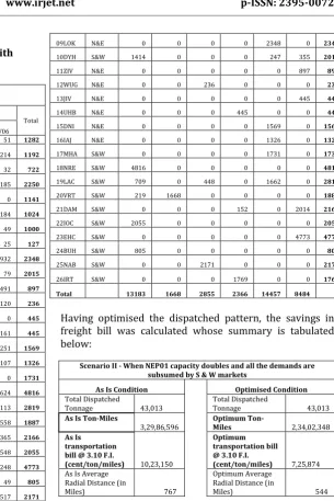
Having optimised the dispatched pattern, the savings in freight bill was calculated whose summary is tabulated below:
Scenario II - When NEP01 capacity doubles and all the demands are subsumed by S & W markets
As Is Condition Optimised Condition
Total Dispatched Tonnage
43,013
Total Dispatched
Tonnage 43,013
As Is Ton-Miles
3,29,86,596 Optimum Ton-Miles 2,34,02,348
As Is transportation bill @ 3.10 F.I. (cent/ton/miles)
10,23,150
Optimum transportation bill @ 3.10 F.I. (cent/ton/miles)
7,25,874 As Is Average
Radial Distance (in
Miles) 767
Optimum Average Radial Distance (in
Miles) 544
[image:5.595.253.559.69.527.2]Scenario III – When production capacity of NEP01 is doubled, it is assumed that in As-Is condition the increased production would be subsumed by only North and East markets proportionately because of proportionate increase in demand in North and East markets. It was also assumed that the demand of South and West markets would remain unchanged.
Table 8 and Table 9 shows the As-Is and Optimised condition tonnage matrices for this scenario respectively.
Table 8
As-Is Condition (For freight optimisation with enhanced capacity - Scenario III)
Tonnage Matrix showing As - Is dispatch pattern (Average Monthly ‘tons’)
Sales
Hubs Region Manufacturing Locations Total NEP01 WED02 NUK03 RAK04 JAR05 JIV06
© 2019, IRJET | Impact Factor value: 7.34 | ISO 9001:2008 Certified Journal
| Page 843
02CUL N&E 566 47 21 0 791 214 1640
03AHG N&E 118 73 51 0 541 32 815
04AHC N&E 1862 158 43 9 1467 185 3724
05MOB S&W 0 288 190 52 611 0 1141
06NUP S&W 0 79 153 0 608 184 1024
07AOG S&W 321 1 80 16 97 49 564
08GAN N&E 216 8 29 0 20 25 298
09LOK N&E 1416 98 93 16 913 932 3469
10DYH S&W 401 55 322 121 492 79 1470
11ZIV N&E 331 68 43 52 174 491 1159
12WUG N&E 85 16 0 82 120 304
13JIV N&E 269 31 96 121 140 0 657
14UHB N&E 271 25 22 0 181 161 660
15DNI N&E 1013 0 95 0 1012 251 2371
16IAJ N&E 699 147 142 0 784 107 1880
17MHA S&W 336 149 56 0 734 0 1275
18NRE S&W 846 16 286 439 1456 624 3668
19LAC S&W 418 41 146 182 351 1113 2252
20VRT S&W 282 0 197 5 462 558 1504
21DAM S&W 370 78 219 233 399 365 1664
22IOC S&W 267 9 73 311 484 548 1693
23EHC S&W 958 48 188 332 698 1248 3473
24BUH S&W 152 15 168 33 182 49 598
25NAB S&W 345 45 0 230 567 517 1703
26IRT S&W 160 0 132 214 468 579 1552
Total 13183 1668 2855 2366 14457 8484
Table 9
Optimised Condition (For freight optimisation with enhanced capacity - Scenario III)
Tonnage Matrix showing optimum dispatch pattern considering same production capacity of each manufacturing location and same demand of each sale hub
(Average Monthly ‘tons’)
Sales
Hub Region Manufacturing Locations Total NEP01 WED02 NUK03 RAK04 JAR05 JIV06
01LED N&E 0 0 0 0 2454 0 2454
02CUL N&E 0 0 0 1640 0 0 1640
03AHG N&E 0 0 0 0 815 0 815
04AHC N&E 0 0 0 0 3724 0 3724
05MOB S&W 1141 0 0 0 0 0 1141
06NUP S&W 1024 0 0 0 0 0 1024
07AOG S&W 564 0 0 0 0 0 564
08GAN N&E 0 0 0 0 298 0 298
09LOK N&E 0 0 0 0 1640 1829 3469
10DYH S&W 1470 0 0 0 0 0 1470
11ZIV N&E 0 0 0 0 0 1159 1159
12WUG N&E 0 0 304 0 0 0 304
13JIV N&E 0 0 0 0 0 657 657
14UHB N&E 0 0 0 660 0 0 660
15DNI N&E 0 0 0 0 2371 0 2371
16IAJ N&E 0 0 0 0 1880 0 1880
17MHA S&W 0 0 0 0 1275 0 1275
18NRE S&W 3668 0 0 0 0 0 3668
19LAC S&W 2252 0 0 0 0 0 2252
20VRT S&W 0 1504 0 0 0 0 1504
21DAM S&W 773 0 0 0 0 891 1664
22IOC S&W 1693 0 0 0 0 0 1693
23EHC S&W 0 0 0 0 0 3473 3473
24BUH S&W 598 0 0 0 0 0 598
25NAB S&W 0 0 1703 0 0 0 1703
26IRT S&W 0 164 848 66 0 474 1552
Total 13183 1668 2855 2366 14457 8484
Having optimised the dispatched pattern, the savings in freight bill was calculated whose summary is tabulated below:
Scenario III - When NEP 01 capacity doubles and all the demands are subsumed by N & E markets
As Is Condition Optimised Condition
Total Dispatched
Tonnage 43,013 Total Dispatched Tonnage 43,013
As Is Ton-Miles 3,43,42,35
4 Optimum Ton-Miles 2,26,35,547
As Is transportation bill @ 3.10 F.I.
(cent/ton/miles) 10,65,202
Optimum transportation bill @ 3.10 F.I.
(cent/ton/miles) 7,02,090
As Is Average Radial Distance (in
Miles) 798
Optimum Average Radial Distance (in
Miles) 526
Inference: Summary of the transportation bills in all 3 scenarios are tabulated below:
Transportation Bill
As Is Condition Optimised Condition
Scenario I 10,34,229 7,15,495
Scenario II (S&W) 10,23,150 7,25,874
Scenario III (N&E) 10,65,202 7,02,090
From the above table, we can see that Scenario III in the optimised condition has lowest freight bill. Thus, company would be most benefitted if demand rises specifically in North and East regions to consume entire additional production from NEP01 manufacturing location.
In this context, it is interesting to note that Scenario III had highest freight bill in As-Is Condition. This might be due to the fact that North and East regions are farther away from the manufacturing location NEP01.
© 2019, IRJET | Impact Factor value: 7.34 | ISO 9001:2008 Certified Journal
| Page 844
Our second observation is that the difference between highest freight bill and lowest freight bill in As-Is Condition is USD 42,052. This reduces to USD 23,784 in optimised condition. Thus, no matter which demand scenario emerges in future, difference in freight bills would not be significant.
Besides, since Scenario I is the most likely scenario, the intensity of risk of higher freight bill is only USD 13,405. So, management can safely opt for increasing the capacity utilisation in NEP01 manufacturing location.
Optimisation of Contribution Margin
While optimising the freight network, it was realized that the company is realizing different margin for different products in different markets. Therefore, an optimisation analysis to maximize the overall margin of the company from the market was also carried out.
To carry out this analysis, the data were organised in the following format:
Contribution Margin = Realised Selling price – Variable cost of product in the market.
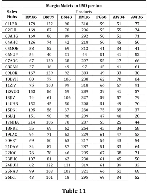
Margin Matrix: This matrix contains the margin on different products in different markets (Table 10).
Tonnage Matrix: This matrix contains the total dispatched quantities in tons from each manufacturing location to respective sales hub during a month (on average) (Table 11).
After arranging data in such format, we optimised the dispatch pattern from each manufacturing location to all sales hub by using Network optimisation technique. While optimising the dispatch pattern following assumptions were made:
I. Total production capacity of a manufacturing location for a product was considered constant. II. Total demand of each sales hub was considered
constant.
Although, this analysis had been carried out for all the manufacturing locations, but for the sake of simplicity, we are producing data of the manufacturing location with highest potential. Product wise details of all manufacturing locations would have been too cumbersome to be included in this note.
In this case study, we found that margin was not only dependent on freight, but it is a factor of following parameters, among others:
I. Freight: Lower the freight from the manufacturing location, lower the landed cost of product and hence higher margin
II. Competition: Less presence of competitors in a market, higher the margin, since supply creates pressure on price
III. Local taxes: Higher the local taxes, lower the margin
IV. Relative cost of manufacturing at different manufacturing location: If two manufacturing locations serve the same market, one with lower cost of manufacturing would fetch better margin Considering all these factors, the analytical tool called ‘Solver’, calculates optimal scenario showing which manufacturing location should serve which market to maximise the margin.
The optimised margin matrix is shown in Table 12.
Table 10
Margin Matrix (For Margin Optimisation study)
Margin Matrix in USD per ton Sales
Hubs
Products
BM66 BM99 BM43 BM16 PG66 AW34 AW36
[image:7.595.310.556.326.650.2]01LED 179 122 90 310 59 51 77 02CUL 169 87 78 296 55 55 74 03AHG 169 86 89 292 50 51 71 04AHC 126 74 42 218 50 45 50 05MOB 58 82 69 312 41 34 41 06NUP 54 40 31 44 51 41 52 07AOG 67 130 38 297 55 17 66 08GAN 37 16 49 97 45 41 61 09LOK 167 129 92 303 49 33 30 10DYH 80 77 106 238 62 70 84 11ZIV 75 108 99 318 66 67 91 12WUG 153 86 59 289 39 41 57 13JIV 74 61 106 327 59 57 79 14UHB 152 45 50 208 51 49 70 15DNI 195 58 37 230 75 35 37 16IAJ 151 90 96 299 47 40 20 17MHA 214 106 70 287 55 25 44 18NRE 55 69 62 264 45 34 58 19LAC 94 71 62 229 61 47 53 20VRT 69 50 63 217 54 43 54 21DAM 34 87 57 287 51 33 64 22IOC 76 78 46 295 67 38 71 23EHC 107 81 62 230 61 45 58 24BUH 62 122 111 319 61 39 33 25NAB 99 103 103 321 66 51 68 26IRT 43 101 18 295 69 34 52
Table 11
As – Is Scenario (For Margin Optimisation study)
Tonnage Matrix showing As is Dispatch in ton
Sales Hub
Products Total
BM66 BM99 BM43 BM16 PG66 AW34 AW36
01LED 114 31 - - 22 69 20 257
02CUL 47 11 - - 107 - 20 185
03AHG 3 - - - 17 - - 20
© 2019, IRJET | Impact Factor value: 7.34 | ISO 9001:2008 Certified Journal
| Page 845
05MOB 1,530 274 8 29 763 174 750 3529
06NUP 1,523 115 5 8 899 299 287 3135
07AOG 540 48 2 6 130 65 151 942
08GAN 18 - - - 9 14 12 52
09LOK 127 34 1 - 206 25 112 504
10DYH 212 45 2 4 16 140 179 597
11ZIV 21 3 0 2 24 36 52 138
12WUG 36 - - - 19 6 - 61
13JIV 82 - - - - - - 82
14UHB 19 - - - 43 - - 63
15DNI 23 13 0 27 57 9 109 238 16IAJ 14 1 7 - 3 31 61 117 17MHA 61 37 8 7 9 36 43 201 18NRE 532 62 7 0 134 60 50 846 19LAC 249 4 1 0 37 32 3 326 20VRT 194 - - - 150 - - 344
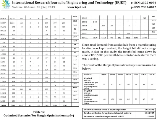
[image:8.595.30.562.47.452.2]21DAM 464 43 10 10 120 41 192 880 22IOC 281 2 7 - 5 4 8 307 23EHC 611 369 18 11 275 14 137 1435 24BUH 212 2 - 4 5 7 36 265 25NAB 349 13 4 2 72 75 143 657 26IRT 178 1 - 0 49 19 21 268 TOTAL 7530 1112 82 112 3202 1181 2502 Table 12 Optimised Scenario (For Margin Optimisation study) Tonnage Matrix showing Optimised Dispatch in ton Sales Hub BM66 BM99 BM43 Products BM16 PG66 AW34 AW36 Total 01LED 257 - - - - - - 257
02CUL 185 - - - - - - 185
03AHG 20 - - - - - - 20
04AHC 274 - - - - - - 274
05MOB 2,848 - - 112 - 569 - 3529
06NUP - - - - 2,921 214 - 3135
07AOG - 942 - - - - - 942
08GAN - - - - - - 52 52 09LOK 504 - - - - - - 504
10DYH - - - - - 398 198 597 11ZIV - - - - - - 138 138 12WUG 61 - - - - - - 61
13JIV - - - - - - 82 82 14UHB 63 - - - - - - 63
15DNI 238 - - - - - - 238
16IAJ 117 - - - - - - 117
17MHA 201 - - - - - - 201
18NRE - - - - - - 846 846 19LAC 326 - - - - - - 326
20VRT 344 - - - - - - 344
21DAM - - - - - - 880 880 22IOC - - - - - - 307 307 23EHC 1,435 - - - - - - 1435
24BUH - 169 82 - 13 - - 265
25NAB 657 - - - - - - 657
26IRT - - - - 268 - - 268
TOTAL 7530 1112 82 112 3202 1181 2502
Since, total demand from a sales hub from a manufacturing location was kept constant, the freight bill did not change much. In fact, in this study, the freight bill came down by almost USD 5000 per month because in ton-miles terms there was a saving.
The result of the Margin Optimisation study is summarised as below:
Products: BM66 BM99 BM43 BM16 PG66 AW34 AW36
Weighted average contribution, per ton, for as is dispatch pattern (USD)
72 82 65 257 51 43 52
Weighted average contribution, per ton, for optimised dispatch pattern (USD)
101 129 111 312 53 47 67
Total contribution for as is dispatch pattern: 1,015,891
Total contribution for optimised dispatch pattern: 1,341,957
Increase in contribution per month in USD 326,066
3. CONCLUSIONS
We are fully conscious of the fact that the result of this analytics shows an ideal final result (IFR). However, in practice, the company might face some constraints while practically implementing the entire recommendation.
Therefore, a series of brainstorming sessions between interfacing departments were held leading to a number of action items which finally resulted in considerable cost saving and margin improvement for the company. The major changes brought about were related to following aspects:
Change of product mix of various manufacturing locations.
Change of product mix in various markets.
Construction of a new manufacturing location in a geographical region which had high demand and had locally available raw material but no manufacturing location.
A number of recipe optimisation study were also carried out to reduce the inbound transportation cost.
© 2019, IRJET | Impact Factor value: 7.34 | ISO 9001:2008 Certified Journal
| Page 846
REFERENCES
[1] Pragnya Parimita Mishra, Kunal Sharma, “Inventory and Logistics Cost Optimization in Automobile Industry”,
International Journal of Engineering Research and Applications (IJERA), ISSN: 2248-9622, Vol. 3, Issue 4, Jul-Aug 2013, pp.1632-1635.
[2] Craig, Don. “What is Supply Chain Network Optimization?” TransportationInsight (blog), June 10,
2014, //
www.transportationinsight.com/blog/networks/2014/ 06/supply-chain-network-optimization/.
BIOGRAPHIES
Sanjeeva, Bachelor of Technology from Indian Institute of Technology (ISM) Dhanbad, India, MBA from S P Jain Institute of Management and Research, Mumbai, India, Six Sigma Black Belt, presently working as President (Commercial & Special Projects) in a leading building material company in India.