Autonomous Decision Making for a Vehicle
Isha
Student
National Institute of Technology Kurukshetra, India
Mamtesh
Assistant Professor National Institute of Technology
Kurukshetra, India
ABSTRACT
It includes Deep Learning techniques using convolutional neural networks for getting the predictions and probabilities for the best decision that has to be made while driving a car like lane detection, traffic signals recognition and their localization and simultaneously developing a steering model to help to take decision regarding steering wheel, throttle thus stimulate a car like humans. In this paper, lane detection is the main concern is to move the steering in appropriate direction with proper angle and the problem is solved using convolutional neural networks via creating a model which then is trained over some collected training data of steering decisions on a track in a simulated environment.
Keywords
Autonomous Car, Autonomous Vehicle, Driverless Cars, Deep Learning, Convolutional Neural Network
1.
INTRODUCTION
In the world of improving technology day by day self driving cars are one of the booming side of the technology empowerment while during driving it is must that the driver must pay his/her complete attention to minimize the risk of accidents which is for sure a tiring task and since computers can make computations, calculations and processing faster than a normal human thus it can surely serve benefit in making decisions in some day to day activities such as driving. It can also help in optimizing fuel consumption by calculating shorter paths and being in disciplined manner while driving. This paper is associated with Deep Learning and convolutional neural networks[11][17] to create an autonomous decision maker for vehicles which can do all the necessary calculations and computations and processing such as being in right lane, identify traffic symbols and the main thing which is steering control help a vehicle to drive as like a human is driving it such a methodology have helped us to greatly improve the visual traffic symbol recognition, object localization and detection and simultaneously other corresponding domains including self driving vehicles[1] etc. There are mainly two modeling strategies. Earlier traditional system does a lot of computations in order to find out what would be the steering predicted angle and real time image is captured from the cameras that are being fitted all over the car to get the required complete overview of car surroundings. But in end to end systems, we only need to take the data in front of vehicle and from it give out a steering angle. Although using end to end models for real self driving car requires a lot of labeled data which is still not present according to Andrew Ng [3][4]. But their performance can be seen on demo systems. In this paper, implementation is divided into 3 aspects:
Lane detection part which concerns with detecting the lanes on the roads and highways which becomes the foremost part of the implementation via which one can come up with a decision to be in right lane while driving always. Also there is a challenge with the curvy roads which can be tackled bird eye view and sliding window approach to get the resulted line describing the interested lane.
Traffic sign recognition- The objective of this module is to recognize traffic signs so that rules should be followed by autonomous car.
Predict the angles at which the car needs to be moved similar to what a human would do.
The remaining sections of this paper are as follows. Section 2 discusses about the literature survey of autonomous cars. Section 3, 4, 5 about implementation. Section 6 represents the result and observations. Finally section 7 discusses about the limitations of the current work, and covers the future directions of this work.
2.
BACKGROUND
2.1
Convolution Neural Network
[image:1.595.317.542.488.664.2]Convolutional neural network is also a category of neural network [1] with some added layers. These are vital in order to process an image including in it are Convolutional layer, non linearity, pooling and fully connected layer[3][13].
Fig 2.1: Convolutional Network [3]
Convolving Step
In above figure, Image is converted in set of pixels and on it filter is moved which is given by:
1 0 1
0 1 0
1 0 1
The filter is of dimension 3x3.Above given image sample is of dimension 5x5 and the output will be of dimension (n-f+1). * (n-f+1) . where n is size of image and f is size of filter ,i.e. (5-3+1) x (5-3+1) which is equal to 3x3. Here the value of one cell of convolved feature is defined by element wise multiplying the filter with the image on which it is currently present and adding those numbers together.
[image:2.595.82.256.74.173.2]Padding can also be useful in order to put off the removal of important features from border after adding a padding of p, output will be of dimension (n-f+2*p+1) * (n-f+2*p+1). Stride can also be included to this which defines step width ((n+2*p-f)/s)+1 * ((n+2*p-f)/s)+1
Fig 2.2: Convolution over Volume
Non Linearity
If non linearity is not functional, the output will be reliant upon the input in a linear form and thus it hysterics the data almost linearly and it is of no use in case if we use large amount of layers.
Pooling Layer
It reduces size of output layer height and width, as it just extracts features which is required from a particular region ignoring other. Pooling Layer[16][15] can be of 2 types: Max and average Pooling. In max pooling, there is a window of some resolute size and it is moved over the output of previous layer and this window finds out the maximum value inside the existing window. In average pooling, we take the average of the current window. There is no trainable parameter in this window.
Flattening the Layers
After finishing the previous steps, we supposed to have a pooled feature map by now. In this step convert the matrix into 1-D array.
Fully Connected Layer
This is the final layer responsible for decision making and produces output just similar to neural layers. The trainable parameters between these layers are given by Nneurons in current layer * Nneurons in next layer. Output can be softmax layer in case of classification problem statement or regression output.
3.
ADVACNE LANE DETECTION
The one of the most required activity in driving a car is to be in right lane to avoid any mishappening, thus one of the main concerns becomes to detect the lane so that the automated car can run in a prescribed area and avoid accidents. This approach is used to minimize the errors as much as possible. The detailed procedure of identifying lane is described as below.
[image:2.595.318.546.269.410.2]The following picture describes with what we are going to start
Fig 3.1: Picture of Unprocessed Image
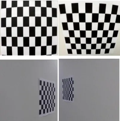
[image:2.595.329.530.550.753.2]Camera Calibration: In the real world when a picture is captured in camera there comes distortion due to conversion of 3D plane in 2D plane. The algorithm where image is converted from 3d to 2d, suffers dilemma of winding at edges. Therefore, first step in detecting lanes become calibration of camera[5][6]. This progression involves calculating point on image and point on real object in 3d plane object of predefined form of a chess board, the reason it uses a chess board is that a chess board has a preset shape and we can easily judge when it is distorted. Around 20 pictures are picked from a chess board which is taken from unusual angles.
Fig 3.3: Finding Points on Image
Pseudo code for camera calibration is
def find_corners(array_of_chessboard_images)
start
for every image of chessboard used for calibration
objectpoints=create a grid of points like in the 3d space (0,0,0),(0,1,0)…(8,5,0) where z always zero as 2d
imagepoints=find_Chessboard_Corner(image,(points_in _x_dir,points_in_y_dir))
save imagepoints and objectpoints in the list
return list
end
Distortion Removal: The next step is distortion removal. Since due to tilting and various angles at which picture is taken distortion is introduced. Using points calculated in earlier step, calibration is achieved. It results in some matrix and vectors which helps to map one type of points on actual object to points on an image for every further image that we wish to correct.
function
undistort_image(image,imagepoints,objectpoints)
#caliberate_Camera using imagepoints and objectpoints
#camera matrix that is used to transform 3d image to 2d image
#distortion vector that consist of 5 vectors that is used to correct the distortion in an image
vectors,matrix=caliberate_Camera(imagepoints,objectpoi nts,image_shape)
#undistort image using camera matrix and distortion vector
[image:3.595.332.528.189.421.2]return undistort (image,mtx,dist)
Fig 3.4: Distortion Removal Over a Sample Image
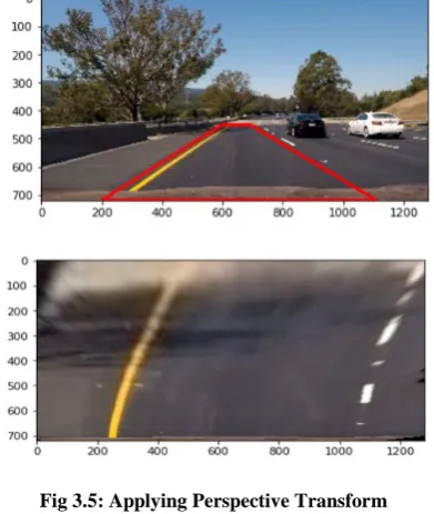
Perspective Transform: Since camera is recording from front, the lanes appear to converge at far distance due to which curvature recognition becomes difficult.. Actual lanes are parallel but due to this distance and shape size proportionality they appear to meet at far distance which created difficulties for identifying the lane and its curvature. Therefore there is needed to look it from some different perspective where they still appear parallel. The best Perspective is to stare from top which is recognized as bird eye view.
Fig 3.5: Applying Perspective Transform
Pseudo Code:
function transform_perspective(image,S_points, D_points)
start
#here source_points and destination_points are point on a real and wraped image respectively
#source_points and destination_points representing a polygon
matrix=find_matrix_for_transformation(source_points,de stination_points)
bird_eye_view=apply_perspective_on_image(image,mat rix)
return bird_eye_view
end
[image:3.595.64.279.646.724.2]Fig 3.6: Poor Separation of Lane Lines in GrayScale
[image:4.595.319.546.71.533.2]Fig 3.7: Thresholding on Red Channel
Fig 3.8: Best Detection in Saturation Channel ofHLS
Pseudo Code:
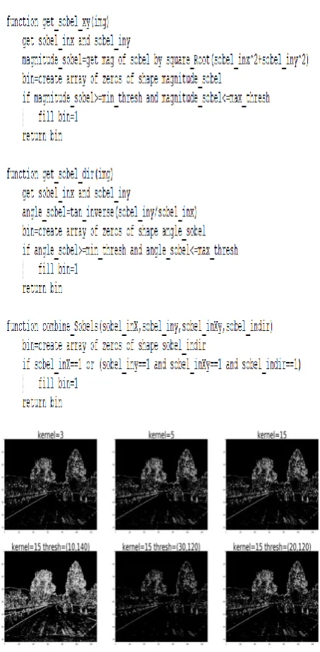
Gradient Thresholding: For images with poor and non-uniform illumination, gradient thresholding is required to separate the objects of attention from the background.
Now to find sudden changes in the input frame which is edges Sobel transform is used[8]. Here combination of x, y, xy and directional Sobel is used. Directly canny edge is not used because Sobel gives us flexibility to find edges with directionality and intensity constraint which removes unwanted edges and give a more specific filtering.
Pseudo Code:
[image:4.595.58.287.72.417.2]Fig 3.9: Experimenting Various Threshold and Kernel Parameters for Sobel x
Fig 3.10: Directional Thresholding Parameters Experimentation
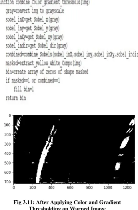
[image:4.595.322.551.571.712.2]Pseudo Code:
Fig 3.11: After Applying Color and Gradient Thresholding on Warped Image
Drawing histogram: Histogram of perspective image is drawn by summing pixels of y direction and peaks of histogram shows the x positions where lane lines are present. Because the intensities at that position will be maximum.
Pseudo Code:
function find_histogram(image)
/* function to create histogram based on intensities in y direction*/
Cropped=image[(height//2):,:]
#crop image and get bottom half image
hist=calculate sum on vertical axis i.e axis=0 with sum function return hist
Fig 3.12: Identification of Lanes Using Histogram
[image:5.595.59.280.87.424.2]Sliding Window: X position from drawing histogram gives starting position for applying sliding window approach. This approach helps to find white points which are present under the sliding window. The output of this step is points under sliding window which is likely to be a part of lane line
Fig 3.13: Application of Sliding Window Approach
Fitting Polynomial: After getting the points of lanes from sliding window approach a 2nd degree polynomial is fitted to coordinates of points founded which will give a clear line of lane identified after the processing the image which the major goal of the lane detection. The complete procedure is done once only because lines mostly remain same and previous curve can give us wide information about new curve
Pseudo code:
function lane_fit(image) start
hist=find_histogram(image)
left_start,right_start=find_peaks(hist)
set parameters for sliding window
non_zero=find nonzero points
if initial_info_present then
left_fit=A*(nonzero_y)^2+B*nonzero_y+C
left_lane_inds=inds of non-zero points present within a margin from left_fit
right_fit=A’*(nonzero_y)^2+B’*nonzero_y+C’
right_lane_inds=inds of non-zero points present within a margin from right_fit
percentage_of_points_inside_sliding_window=((sum(left _lane_inds)+sum(right_lane_inds)) //len(nonzero)
if percentage_of_points_inside_sliding_window<req_per or no previous information then
for w in range 0 to(no_of_total_windows-1)
calculate dimensions of current window
sliding_left=save inds from nonzero which is present under sliding window moving on left_lane
sliding_right=save inds from nonzero which is present under sliding window moving on right_lane
append these points to the left_lane_inds and right_lane_inds respectively
if len(sliding_left)>min_pixels:
#determiningstart for next window to accommodate curving of lanes
left_lane_start=mean of dimensions of points under left_lane
if len(sliding_right)>min_pixels:
[image:5.595.61.278.590.689.2]#fit_2_degree curve on left lane with x axis as y_left and y axis as x_left
left_fit=polyfit(y_left,x_left,2)
right_fit=polyfit(y_right,x_right,2)
#save information of curve and nonzero points and dimensions of sliding window in left_lane_info and right_lane_info
return left_line_info,right_lane_info
Additional information: Radius of curvature is calculated which is an essential measure for driving cars. Formula used is called curvature formula.
R= [1+(y’(x))2
]3/2 /|y’’(x)|
Here y(x) is the 2 degree polynomial
y`(x), y``(x) is single derivative and double derivative respectively
[image:6.595.58.279.296.486.2]R is radius at point y=point at foot of road
Fig 3.14: Final Output of Detected Lane
Old versus New Approach Output Comparison
[image:6.595.331.524.334.576.2]This approach is advance version of the approach discussed in minor project. The output of earlier approach looks like below
Fig 3.15: Minor Project Approach of Lane Detection
Some differences in output are as follows:
In earlier version, A 1d line of type y=mx+c is fitted and simple image processing techniques are used to detect them. But in advance version a quadratic function is used to fit the lines with some advance algorithms which seems to be a better fit for the lane lines
Lane fitting in earlier version does not do that much great on curves and these lines seem to merge together.
Therefore, In the new approach the lane lines are fitted from different angle like viewing from above to better detect lines which appear to meet at end of road but in actual they are parallel which can be easily viewed If it is looked from above
In current version more advance metric calculation can be done like calculating twist, but this can’t be achieved in earlier version.
A better and smooth fit is obtained in current version as compared to previous versions
4.
END-TO-END DECISION MAKING
FOR STEERING ANGLES
Main important part of self driving car is to predict the angles at which the car needs to be moved similar to what a human would do.
Data Collection
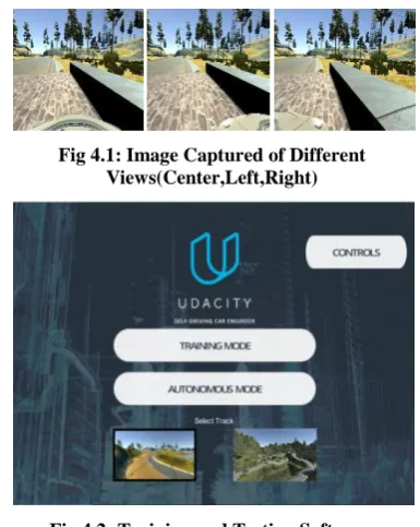
In this paper, data is collected by actually driving the car in the training mode given in the software. The collected is stored in a .csv file having seven columns, first three columns provides the link for the left, right and center captured images, a column for steering angle, throttle, brake and speed is stored. .
Fig 4.1: Image Captured of Different Views(Center,Left,Right)
Fig 4.2: Training and Testing Software
Data Balancing
[image:6.595.55.286.531.650.2]trained on the data with lot of left right steering then the car will not travel straight even on a straight road because it will learn to rotate the steering as much as it learned from left and right steers during the training. The problem arises due to this is that the car would not be able to travel along a straight line and keep on deflecting from the required lane which can surely increase the chances of sever accidents and hence this is why we need to balance the data. There are two techniques used to balance the data in this project which are discussed as below.
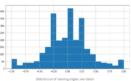
[image:7.595.326.536.139.269.2] Advanced Data Collection Technique: In this technique the goal is to collect data in a smart way such that it balances the data according to the requirements. This is achieved by collecting the data at some particular locations of the track.
Fig 4.3: Visualization of Data Collected (nearly centralized to zero degree)
Now to eradicate this problem the strategy made was to increase the data at which steering is at some angle and to do so the car at data collection mode of simulator was drove randomly at left and right angles of steering even on the straight road as a result of which they get data rid of biasness around zero degree. Now again as a problem the car started moving not in a straight even at the straight road. Thus to get rid of all this data is balanced precisely over a particular values. Data augmentation is performed which is discussed later. Thus via this technique data balancing can be achieved and this is how the dataset is improved to required extent.
Data Augmentation: End to end system works better with a lot of data more good therefore in order to reduce the biased parts in order to prevent the network to always at 0 angle we add different augmentation[9] techniques. Here we have used left and right view as also a part of dataset with same steering angles but with little changes done to it to encounter their views. Then the image is flipped using horizontal axis and steering angle is made negative to accommodate the change which in turn can create more data for the particular side. After this image is translated i.e. pixels are moved and depending upon pixels that is moved steering angle is changed according to it. Then random brightness is provided to image by converted image into HSV and changing its V component. Also random shadow is applied by converted image into HSL and changing light component of image and hence a lot of translations, transformation are applied to balance the data. Data augmentation can be proved a best technique to generate data at runtime which is used up and destroyed after usage at the run time as well. This is effective approach as it can overcome the problem of
[image:7.595.57.279.208.393.2]memory as well. Using data augmentation drastic changes to the dataset has been observed which is favorable to the project as it remove completely the problem of data centralization over zero value and proved to be good technique for run time data creation and memory constraints.
Fig 4.4: Data Balancing via Data Augmentation
5.
TRAFFIC SIGNAL DETECTION
Traffic signs are an important part of road understanding and autonomous and instantaneous decision making. Without these signs the probabilities of road accidents will escalate. So to further improve the functionality of our model, we have introduced this essential and vital feature called Traffic Sign Detection. In this paper, German traffic signs are used which basically have 43 classes of various traffic signs viz.
Fig 5.1: Random Samples from Training Set One from Each Class
The objective of this module is to recognize these traffic sign and classify them based on classes to which it belongs First step for this is to preprocess the images using following methods as given in research paper [12]
Changing the color schema from RGB to YUV. Here we convert the 3 channeled RGB image into YUV where only Y channel is used.
Changing image contrast suitably. Some images contrast is not upto mark, So to enhance this its contrast is enlarged by means of Histogram Equalization.
Standardizing or Normalizing Image is normalized to improve optimizer rapidity for convergence. For this, Mean is subtracted and divided with its standard deviation.
Model Architecture
[image:7.595.325.540.411.544.2]as non linearity constraint.2 FCC layer is employed having softmax output of 43.Gradient Descent is used as a method to reduce loss. This model produces following accuracy
Output accuracy for this is not up to mark. So we moved to more complex model, changing basic lenet, adding more deepness and layers to network and also data augmentation is also employed. A more advance optimizer i.e. adam optimizer is used to train model. The architecture is shown below
This modified model helps to improve the accuracy up to 98% Following method is used to augment our images.
[image:8.595.314.542.72.269.2]Data Augmentation Various data augmentation techniques as mentioned in that section are applied to get an array of randomly plotted images. Datasets of images are generally big. So storing them is a challenging task. Also it solves the issue of data imbalance across classes. Here data becomes highly varied which cover general real time conditions. So we use data augmentation here to generate many augmented images at runtime for training. Image data generator of keras is used for this point.
Fig 5.2: Sample Augmented images
6.
RESULTS AND OBSERVATIONS
6.1
Steering Decision
The automated car is able to take decision based on the runtime input frames and able to travel properly on the required track in the simulated environment. The steering decision can be viewed on the terminal screen and collaborated with simulator the car can run.
Fig 6.1: Self Driving in Action
6.2
Lane Detection
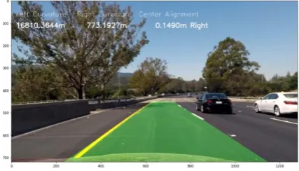
[image:8.595.55.285.333.447.2]The final lane is detected successfully and is bounded in a green region depicting the required results. The curvature too is calculated successfully using the formula mentioned in the description of lane detection module along with the information of alignment of the car from the center of the lane. The final output of the lane detection module is shown as below
[image:8.595.322.536.627.749.2]6.3
Traffic Sign Classifier
The implemented model is successfully able to classify the input traffic signs with an accuracy of nearly 98%.
7.
CONCLUSION
Traditional systems do not have capability to take decision on such various parameters and to slow run time capabilities and memory constraints the challenge become more difficult. The field of automation does a lot of computations in order to find out what would be the predicted angle for the steering. In earlier systems, the direct work is on the real time image that is being captured from the cameras integrated with the sensors which are being fitted all over the car to get the complete overview of the surroundings in which car is traveling. The information collected from these sensors is applied together and get fused in order to produce a meaning full output of the types of object in surrounding of the vehicle and also detect where the lanes are present so that vehicle can stay on road. Along with all this it needs to detect and decode the meaning of the traffic symbols which needs to be followed. Although using end to end models for real self driving car requires a lot of labeled data which is still not present this is according to Andrew Ng. But surely their performance can be measured and seen on the demo systems. In this paper practice of end to end self driving car representation taken from nvidia and then tried to implement a few important components that are useful in actual systems which includes lane detection and traffic sign classifier which can be moreover combined with sensors fuse the information and path planners to detect the actual angle which satisfies the main aim of the paper
.
8.
REFERENCES
[1] Brilian Tafjira Nugraha, Shun-Feng Su, Fahmizal et al., “Towards Self-driving Car Using Convolutional Neural Network and Road Lane Detector”, 2nd International Conference on Automation, Cognitive Science, Optics, Micro Electro-Mechanical System, and Information Technology (ICACOMIT), IEEE, 2017.
[2] Mochamad Vicky Ghani Aziz, Ary Setijadi Prihatmanto, Hilwadi Hindersah et al., “Implementation of Lane Detection Algorithm for Self-Driving Car on Toll Road Cipularang using Python Language”, 4th International Conference on Electric Vehicular Technology (ICEVT), IEEE, 2017.
[3] LecunY, Bottou L, Bengio Y, et al.”Gradient-based learning applied to document recognition”, Proceedings of the IEEE, pp-2278-2324,1998
[4] Davida Del Testa, Daniel Dworakowski, Jiakai Zhang et at., “End to End for Self Driving Cars”, Nvidia Corporation Holmdel, NJ 07735, 2016.
[5] Zhang, Zhengyou et al., "Camera calibration with one-dimensional objects." IEEE Transactions on Pattern Analysis and Machine Intelligence, pp 892-899, 2004
[6] Zhang, Zhengdong, Yasuyuki Matsushita, and Yi Ma. et al., “Camera calibration with lens distortion from low-rank textures." CVPR 2011. IEEE, 2011.
[7] Gao, Wenshuo, et al., "An improved Sobel edge detection.", IEEE 2010 3rd International Conference on Computer Science and Information Technology, Vol. 5, 2010.
[8] Vincent, O. Rebecca, and Olusegun Folorunso.et al., "A descriptive algorithm for sobel image edge detection.", Proceedings of Informing Science & IT Education Conference (InSITE). Vol. 40. California: Informing Science Institute, 2009.
[9] Nan, Liangliang, and Peter Wonka, et al., "Polyfit: Polygonal surface reconstruction from point clouds.", Proceedings of the IEEE International Conference on Computer Vision, 2017.
[10] Wang, Jason, and Luis Perez et al., "The effectiveness of data augmentation in image classification using deep learning." Convolutional Neural Networks Vis. Recognit , 2017.
[11] [Rausch, Viktor et al. "Learning a deep neural net policy for end-to-end control of autonomous vehicles.”, 2017 American Control Conference (ACC) IEEE, 2017.
[12] Pierre Sermanet and Yann LeCun et al., “Traffic Sign Recognition with Multi-Scale Convolutional Networks”, Courant Institute of Mathematical Sciences, New York University
[13] Neena Aloysius and Geetha M,” A Review on Deep Convolutional Neural Networks”, International Conference on Communication and Signal Processing(IEEE), pp-588-592, 2017
[14] R. C. Gonzalez, "Deep Convolutional Neural Networks", in IEEE Signal Processing Magazine, vol. 35, no. 6, pp. 79-87, Nov. 2018
[15] S. Albawi, T. A. Mohammed and S. Al-Zawi, "Understanding of a convolutional neural network," 2017 International Conference on Engineering and Technology (ICET), Antalya, pp. 1-6, 2017
[16] S. Lu, Z. Lu, S. Aok and L. Graham, "Fruit Classification Based on Six Layer Convolutional Neural Network," 2018 IEEE 23rd International Conference on Digital Signal Processing (DSP), Shanghai, China, pp. 1-5,2018.
![Fig 2.1: Convolutional Network [3]](https://thumb-us.123doks.com/thumbv2/123dok_us/9301883.429366/1.595.317.542.488.664/fig-convolutional-network.webp)