Performance evaluation of the national bureau of standards implementation of the open systems interconnection class 4 transport protocol in a wide area network environment

Performance Evaluation

of the National Bureau of Standards Implementation

of the Open System Interconnection

Class

4

Transport Protocol

in a Wide Area Network Environment

by

William John Chimiak

Center for Communications and Signal Processing Department of Electrical and Computer Engineering

North Carolina State University

~-\RSTR.-\CT

CHL\1I.AK,

\VILLL~vI JOH~. Performance Evaluation of the

National

Bureau of Standards Implementation of the Open System Interconnection Class 4 Transport Protocol in a "Vide Area Network Environment.

(lJnder the direction of "Y. Chou and 4~.A.Nilsson)

The National Bureau of Standards Implementation of the Open System Inter-connection Class 4 Transport Protocol in a Wide Area Network can be modeled by constructing a two node BC~/fP network with the local operation of the transport protocol represented by an

:vI/GIl

processor sharing node and the external service by an ~l/G/J:. node. The outputs of the model are the service time of the local transport entity and the the time of external service which sum to the time delay introduced by the transport protocol. In reality, the local service time is insignificantly small compared to the total time delay. Development of this model revealed that an assumption of an error free wide area network was unnecessary and that the model deals with realistic degrees of error.

The transport protocol under study is assumed to be resident in the operating system kernel. This permits rapid dissemination of protocol commands with respect to the network layer's support. Therefore, management of the lower layer by the transport entity is the key issue impacting the performance of the transport protocol.

TA-\RLE

OF'

(tO~TE~TS

1 l~TRODlJCTION 1

2

THE OSI ,,"-RCHITECTURE

.

2.1 The OSI Transport Layer 5

2.2 The NBS Transport Protocol 7

2.2.1 Characteristicsof the NBS Implementation 8

2.2.2 Transport Protocol Data Units 9

2.2.3 Datagram Service 10

2.2.4 Transport Service Data Unit Classes 10

3

"~N,,L\.LYSIS OF END- TO-END PROTOCOLS 13

3.1 Introduction 13

3.2 Chapin's Proposed Model 13

3.3 An HDLC Model

0...

14

3.4 Path Control Buffer Overflow Model 14

3.,5 Flow Control Comparison 1.5

3.6 Summary 17

4

j\;IETHOD

OF THE

NBS

TRA2\SPORT

PROTOCOL

.-\~~L\.L

YSIS

18

4.1 Management Concerns of the Transport Protocol... 20

4.1.1 Network Time :20

4.1.2 Impact on Virtual Circuit Service :21

iii

4.1.--1 ~urnrnary of [01pact :2f>

4.1.5

Why Implement the Protocol :26

4 ~) _{Analytical Model -r:}

- I

4.2.1 Assumptions .

... »

o Transport Protocol Model . 29

4.2.2.1 The Processor Sharing Node 3.)

4.2.2.2 The External Node 37

,5 TThfE DEL.L\.)~ -\);ALY-SIS 39

.5.1 Probability that a Service Phase Does not Timeout . Probability the External Service Phase is successful .

:39 43

.5.2.1.1 Expected :\umber of Service Phases 44

.5.3 External Service Time 45

.5.3.1 Introduction 45

.5.3.2 Overhead TPDl~Phases 46

.3.3.2.1 Unlimited Retransmission Assumption 47

.5.3.2.2 Limited Retransmission Assumption 48

.5.3.3 Service Time for the Data Transmission Phases

'so

5.3.3.1 Unlimited Retransmission Assumption .52

.5.:3.3.2 Limited Retransmissions

.

C

.

Wid ~.

,).:3.3.3 Expressions for omposrte v 1 O\V ,_lze . 61

iv

.5.:3.~.1 Datagrarn Probability Density Function 64

5.3.4.2 The Short Transfer 65

5.3.4.3 The Blossomed Transfer 6,)

6

4L\NAL

YSIS OF THE v"ARIOUS NIESSAGE (.TSDU) CLASSES 69

6.1 Successful Virtual Circuit Class (SOLID_ESTAB) 69

6.1.1 External Service Time for the ESTAB Class Message 69

6.1.2 Transport Entity Service Time 71

6.2 Normal Datagram Transactions 71

6.2.1 Two'vVayDatagram Transfer Class (TWO\V~\Y_XFER) .

6.2.1.1 Service Time For Short Transfers .

6.2.1.2 Service Time for Blossomed Transfers .

6.2.1.3 Service Times for the TWOvVA'{·_XFER Class . 76 6.2.2 Three Way Datagram Transfer Class (TRI"V,,~Y_XFER) ; ,

6.2.2.1 Short Transfer Service Time .

6.2.2.2 Blossomed Three Way Datagram Transfer .

6.2.2.3 Service Times for the TRI"V~t\Y_XFER Class ..

;

,

83

84

6.3 Pathological TSDU Classes 85

6.3.1 The Unsuccessful Virtual Circuit Class (NO_ESTAB) 85 6.3.2 Unsuccessful T\\'o \Vay Datagram Class (T'v\tO\V.-\Y_F4~IL) 88

6.:3.2.1 Short Transfer 88

v

6.;3.:2.:~ Total Service Time 9:2

6.3.3 Unsuccessful Three \\lay Datagram Class (TRlv\TA Y_F AIL) 93

6.3.:3.1 Blossomed Transactions 93

6.3.3.2 Short Transfers 93

6.3.3.3 Final TRIW.L~Y_F~\IL Times 97

6.4 Combined ClassesofTSDL~s 98

, RESULTS... 99

8

~-\~ALYSIS

OF RESULTS

104

9

~1~L\.JOR FI);DI:\GS

xxo

Fl~Tl-RE

DIRECTIO:,\S

106

10 REFERE='iCES 109

11 ..L\.PPE~DICES 111

11.1 Appendix ..-\.: Expected ='iumber of External Services... 111 11.2 Appendix B: Service Time of the Second Server 113 11.3 Appendix C: Proof that the datagram b(n) is different from a(n)

114

11.4 APPENDIX D 115

115

11.4.1 Pollaczek - Khinchin .

115

11.4.2 Burke's Output Theorem .

116

11.4.3 Burke's General Output Theorem .

11.4.4 Jackson's Theorem 116

vi

11.4.0 BC'\lP :\et\vorks L17

11.4.6.1 Restrictions: 117

11.4.6.2 Problems Not Applicable to BeMP Solution 117

11.4.7 Arrival Theorem 118

11.4.8 Norton'sTheorem 118

vii

rr

:illLE OF F lGt ·RES

OSI Seven Layer Model 6

Timing Diagram for Transmission Without Transport Layer 22

General Model for TSDU Service 30

Model for a Phase with Only Local Service 31

BC~'1P

Model

of SOI~ID

ESTiV3 Class

TSDlJ 34

General BCNIP Model ofthe Transport Protocol... 36

Data Transfer ~lodel .. 51

EST~-\B

Class .\lessage

Timing Diagram 70

T\VOV\l~-\Y_XFER (Short Transfer) 7:3

T\VO\\l~-\.Y_XFER (Blossomed Transfer) 7-1

BC\tlP ylodel of the Two\\rAY_XFER Class TSDlJ 7.1

TRI'V~~

'{_XFER

(Short Transfer)

78

TRf\V..

AY_XFER

(Blossomed Transfer)

79

BC~lP Model of the TRI"V~-\.Y_XFER

Class Message

80

NO_EST AB Class

TSDU

Timing Diagram

86

BCNIP

~10DEL

OF THE NO_ESTAB

CL~t\SS

TSDU

87

TWOvVAY_FAIL

(Short Transfer) 89

T"VO\V~-\Y_F~t\IL (Blossomed Transfer) 90

BCyIP Model of T"VOW4~)-_F AIL Class Messages 91

viii

TRI\'\P.,-\

)"_F',:\IL [Blossomed Transf'er ) g.)

ix

LlST OF T

~-\BLES

Table 1: Error Free ~et,vorkComparison

Table 2: Network with Error Comparison

100 101 Table 3: Model Breakdown of the ESTAB ClassTSDlJ 102

L

CH.~Tf~R 1

INTRODUCTION

Processing information has always been a hallmark of civilization. Conse-quently, there is always a desire to optimize the ability to process information. Computer communications in the past decade has opened up a major new resource for processing information. This movement has been influenced and directed by the architectures of computer networks.

It is difficult for a single computer manufacturer to offer hardware that is fully suitable for all applications . Assembling a single system which has the greatest generalized power for information processing is a problem which must be solved. It is financially unsound to acquire a separate mainframe computer for every appli-cation. It is also unreasonable to assume that any agency can purvhase every hardware and software suite needed for specialized applications. However. pooling resources to link computing facilities can avoid this problem and prove to be cost effective.

2

and that provides tlexibility for growth which is inciependcnt.of a single mnuufuc-turer. This dissertation focuses on the third approach, the inter-systems communi-cation architecture.

The

Open System Interconnection (OSI) provides the model for such an archi-tecture. OSI is a seven layer architecture. The layered architecture of

OSI

allows an orderly protocol development so long as

the

layer interfaces are well-defined. The structure of its architecture suggests a method of analysis which permits one layer to be distinct from its adjacent layers. This approach provides the first analytical model for the transport protocol which is the lowest layer with true end-to-end significance. Furthermore, because of the layering. t.he methods of analyzing the transport protocol may be applicable to the higher OSI layers.

The National Bureau of Standards (NBS) has implemented a class 4 transport layer protocol. This dissertation analyzes the time delay characteristics of the NBS implementation.

c.

lL\ ~)

rr

ll~

r{

:.?

THE OSI iillCHITECTLrRE

The International Standards Organization (ISO) has developed the Open Sys-tem Interconnection (OSI) reference model to facilitate communication between computer systems. This reference model establishes a seven layer architecture for communication. The layers are the application layer, the presentation layer. the session layer, the transport layer, the network layer, the data link layer. and the physical layer. The ISO study committee 16 has completed the transport layer specification

[1].

From this specification, the National Bureau of Standards (~BS) has implemented a protocol for the OS1 transport layer

[2-4].

This implementation provides two of the five classes of services, the class 4 service and the class 2

ser-VIce.

2.1. OSI Transport Layer

In order to more conveniently discuss the OS1 model, t\VO definitions must be introduced. ~:\. protocol entity is an operational implementation of a protocol. Because there are seven layers in the OSI architecture, some entities in different communicating machines are of the same layer. When these entities communicate

with one another they will do so as peers, being of the same layer. "rhus, they are

peer entities.

Understanding the relationship between the layers of the OSI architecture is a key to understanding rhe transport layer protocol. Figure 1 demonstrates these

relationsh ips.

In the OSI refe-re n ce model, layer ~

(:\i

takes on values 1 through 6) provides layer ~

+

1 with a basic set of functions called service primitives. Furtherrnore, layer ~1 (M = 2,3,-1,5,6) uses the service primitives of layer ~I-l in order to be able

to provide the layer ~{ service prirnitives. So the transport layer, with the network

layer service primitives, supplies the session layer with a basic set of transport

ser-vice primitives.

Peer layer communication is another important concept in the analysis of the

transport layer. Basically, peer entities in the OSI reference model communicate with one another using the services provided by the adjacent lower layers. This

cOffirTIunication may have one of two extents of meaning. The first is end-to-end

significance which involves only the peer entities at both the source and the

UseI"' A

Application

Presentation

Session

Transport

Netwol"'k

Data Link

Physical

1

I

~

."

1

f:::r---J.l

." ~,

J

I

!

I

~, ."

I

Ll

_I

i

i

I

I

I

6

Use!" B ~

7

~igIli li ("an ce. The 0Lher exte ntor conuItUnicatio n iII V()lv(\S Ih(\ 11 ()d(\ (,[ltit i(\S whirh

make up the logical circuit between the source and destination in addition to the

source and destination entities. The layers below the transport layer have protocols with this extent of communication.

Providing transparent end-to-end data transmission to the session layer is the

function of the transport protocol. This function is accomplished using the service

primitives listed

by

the

ISO

study committee 16 in the transport layer specification

[1].

They are:

(1)

connect request indication,

(2)

connect response «onfirmat ion.

(3)

data request indication.

(4:)

disconnect request, and

(.5)

disconnect indication.

Furthermore, the data transmission occurs either through an established logical circuit to the end user, connection-oriented transmission, or to the end user

without previously establishing a logical circuit, the datagram transmission.

2.2. The NBS Transport Protocol

NBS has developed a working implementation of the class 2 and the class!

transport protocols

[2-·4J.

The class :2 protocol is assumed to operate in a very

reli-able network. and the class ,-t protocol is assumed to work in a less reliable

dissertation deals solelv with th« ('la~,~ 1trausport protocol. I"llrtllt,t'lllorl', the sps-sion entity will be referred to as the user, for convenience.

The NBS transport protocol must provide the service primitives in accordance with the formal specification of the transport layer. In order to abstract the ser-vices the transport layer renders for the two different transmission schemes, two

distinct finite state machines (FS~'I) were developed. One was for the

connection-oriented data transfers; the other was for the connectionless or datagram transfers.

2.2.1. Characteristics

or

the NBS Implementation

The resulting '\F~S imploruentatio n has the following characteristics. The

transport entity has a single queue, the work queue. Each transport connection is governed by its own FS~'l. Finally, the entity can be either a user process or be a part of the kernel.

The work queue stores the service phase requests of the transport. service data

units (TSDUs) which are the user requests for transport service. The actual phase of service that the TSDU requires is governed by the connection's FS~'I.

A

separate

FSNI

controls the operation of each transport connection. The

state of the FSN[ isdetermined by the phase of service of the TSDlT and thestatus of the computer system, the network, and the peer entity. Some states call for a

phase of service requiring no external service. These service phases are completed

queue. An example

or

this is the st at.e which closes tht· t.runsport «otuu-ction.

Other states require external service for their associated TSD{}s . The transport entity services these and then sends them out for the network and the peer entity to service. The _disconnect request is one state requiring external service in addi-tion to the local transport entity service.

The .\:BS transport entity can be a user process or a part of the kernel of the operating system. Entities resident in the kernel have priority service. This. most likely, results in the best performance because the protocol functions will enjoy the priority of the operating system instead of a user process priority. The entity created by a user process wou ld be easier to implerne nt because the operating sys-tem would not have to be altered. However, as a user process, this entity would compete with other processes for CPC time.

2.2.2. Transport Protocol Data Units

Transport entities communicate with each other using transport protocol data units (TPDUs). This dissertation deals with six TPDlTs. They are the data (DT), acknowledgement (ACK), connection request (CR), connection confirm (CC), disconnect request (DR), and disconnect confirm (DC) TPDU's.

10

termiuated. The connection is released upon receipt

or

a ()(. "['I-l()lP [rom thv peer

transport entity. In short, the function of a TPDU gives rise to its name.

2.2.3. Datagram Service

The use of the DR TPDU and the DC TPDU differentiates the two datagram service types. The two way transfer is one type. In this service. the user gives his transport entity data in the form of a

TSDlT.

The entity delivers the data with a DR TPDU from the peer transport entity acknowledging the receipt of the TSDL:

and the connection is closed. In the other datagram type, the three way transfer, the

TSDlT

is sent

by

the users transport. entity and is acknowledged

by

the the peer entity. The users trun-sport entity must then acknowledg~the DR TPDLP

with a DC TPDU. This last acknowledgement is the main difference between the two way and the three way datagram services.

2.2.4. Transport Service Data Unit Classes

User requests for datagram and connection-oriented services can be classified. The key to classifying these requests is to trace them through their finite state machines, making note of where significant delays occur. Certain user requests have common delays. Thus, such user requests are grouped in a class. This tech-nique of tracing user requests produced six classes of TSDUs:

:\O_ES'[',\B

TRlvVA.Y_F6..\.IL

TvVOWA Y _XFER

TRIW.A. Y _XFER

II

Con nect ion oriented trunsf'ers whose initinl [Iegotiation parameters are unacceptable to both parties.

Two way datagram transfers whose initial negotiation

param-eters are unacceptable to both parties.

Three way datagram transfers whose initial negotiation

parameters are unacceptable to both parties.

Two way datagram transfers whose initial negotiation par

arn-eters are acceptable to both parties.

Three way datagram t.ransf'ers whose initial negotiation

par arnct crs are acceptable to both parties.

An example of the common delays found for the

NO_ESTi\B

class of TSDU is now

presented.

Example

The following is an example of how the delays are identified for the

~O_ESTAB class of transport request. For clarity, the transport entity initiating

the request, or the sender, is denoted transport

A.

The peer entity responding to the request, or the receiver, is denoted transport

B.

Tracing this class of TSDU through the transport layer yields the following.

(1)

First, the request must be made to transfer data. This results in the user connect request delay. Here the session entity requests the services of the

12

(~) Ir a n e two rk con ne('ti()(L does not e xist , th(' Iirst st ;It. (\ that t~l<• r(Jq11PSt reaches is the CALLING state, which is the wait for a network connection

to be established. This is the network connection confirm delay. Other-wise, the TSDU reaches the CR_SENT state.

(3) Once there is a confirmed network service available, a C~R must be sent by transport A. Transport B sends a CC in response to the CR where the negotiation parameters are not acceptable, as this is a NO_EST AB class

request. So the next delay is the bad connection confirm delay.

(4)

Transport A then sends a DR which is answered by transport B's DC. This is the del ay t0 ~t'Ild a D R.

(5) Transport A waits a reasonable amount of time before releasing the

connec-tion reference number for possible use, where a connecconnec-tion number is a

number assigned by a transport entity to keep control over a given

connec-tion. This is the reference wait delay.

(6) Finally, the connection must be closed which accounts for the closed delay.

( IlL:\~)T EE~. :)

ANALYSIS OF END-TO-END PROTOC·OLS

3.1. Introduction

This chapter presents a su mmary of published studies related to the transport layer. To date. however, only a fe\v papers in the literature deal with end-to-end multifunction protocols. The first models examined are Chapins proposed tran-sport models [.5]. The High-Level Data Link Control

(HDLC)

model of

Bux,

Kum-merle. and Troung [t3J is then d iscussed , followed by Reiser's path control buffer overflow model

[71.

Finally. a review of Sch wartz's work [8] comparing flow con-trol schemes completes the consideration of prior work in the area of end-to-end multifunction protocols.

3.2. Chapin's Proposed Model

For t.he dat.agrurn service, the model proposed by Chnpin dOE's not provide for

the isolation of the transport entity. Instead, he combines the transport entity's queue with that of the network. However, the OSI reference mode] calls for the network layer to be disjoint from the transport layer. Equally important, the NBS implementation does not combine these two queues. Thus, the datagram model cannot be used in this dissertation.

3.3. An HOLC Model

Bux et

al [6]

study the

HDLC

protocol.

In

their paper, they are not concerned with initiation or termination of a connection arid they assume the existence of separate send and receive buffers. Th is model is similar to Chapin's con n--ct ion oriented model and su~ers the same shortcomings. However, only studying the data transfer phase of the protocol is an interesting restriction which this HDLC paper utilizes. Moreover, this strategy does give some indication of throughput restrictions during data transmission.

3.4. Path Control Buffer Overflow Model

In Reiser's paper

[7],

a buffer overflow model is proposed for path control analysis. The operation of a path control scheme in a network is examined. Specifically, Reiser studies the following protocol functions:

15

I~) i L i

\ - flleSS:lges router to ttu en< -usvr [Jro('ess wit hill a dc~tinut.iou uodr.

(3) messages routed on a transit route between nodes of a network,

(4)

implementation of flow con trol, and

(5)

management of the buffer pools.

Reiser studies the behavior of every node In the network. He does not single out

source-destination pairs. As a result, network time is not separated from the total

transaction time. This is not acceptable for the study of the transport layer . ..Another difficulty is that the path control protocol isa function of the System Net-work Archir.ectu re (S.\i~~) of [B~r which does not enjoy a one to one

correspon-dence with the O~l architecture. In particular, Reiser uses a homogeneous network

which has each node actively enforcing flow control. In the NBS implementation,

flow control must be performed by the source and destination transport entities. Reiser's approach, then, cannot be used in the dissertation.

3.5. Flow Control Comparison

A comparison of two flow control mechanisms is the subject of Schwartz's

paper [8]. One mechanism is the swapping window such as that used in SNA

net-works. The other is the sliding window mechanism such as that used in the

tran-sport layer. The study is limited to single, loss-free virtual routes.

The swapping window model is a closed queuing network. It consists of \,1

queues with exponential servers which feed two other components. One is a bulk

If)

the arrival rate of the system. The M queues in this model represents the number

of nodes in the virtual circuit. Because of the bulk arrival mechanism, the Norton equivalent rnethod of solution

[9]

is not applicable. Nevertheless, Schwartz uses

the Norton analysis and compares the results with a simulation of the network.

The results of his simulation shows the Norton approximation to be adequate for

virtual circuits of under six hops with rnoderate loading. At seven hops, even the independence assumption between nodes breaks down which makes the results

worse.

In his sliding window analysis. a closed queuing network is again used . Mes-sages exceeding the available window are assumed to be blocked. His model has :\,

the window size, messages circulating in a closed network of M transit nodes which

ends with a special queue for the window mechanism. The special queue blocks

messages

if

N messages are in the Lv[ nodes. For this model, the Norton

comple-ment queue is solvable using the loss assumption.

This study, then, proposes a heuristic approach for swapping window flow

control schemes. Schwartz uses a loss mechanism which adequately models the

sliding window scheme. The NBS transport protocol, however, is a sliding window

scheme in which messages arriving outside the window are not necessarily lost.

Thus, the swapping window How control model cannot be used as it is a model of a

different flow control discipline, and the sliding window analysis cannot be used as

17

3.6. Surnmar-y

This section dealt with the work related to the study of end-to-end protocols.

None of the four models adequately represents the transport layer protocol. The

next chapter presents a new analytical model as well as the development of the

IS

(

~

u.\

I)

rr

El-{ ~1

iVIETHOD OF THE

NBS

TRf\NSPORT PROTOCOL l\0ii-\L'{SIS

The result of this analysis is an analytical model of the NBS transport layer

protocol in a wide area network envirorunent in which the transport entity under study is embedded in its operating environment. Because the NBS protocol makes

use of only a single queue for holding requests, the transport layer protocol entity

is modeled as a single queue server. The server's output either feeds back to itself,

closes a transport connection, or directs the

TSDlT

to an external server which

feeds the processed TSDl- back to the work que1l€. The external server is made up of the network layer service and the other external transport entities with which

the transport protocol interacts. From this model, an expression for time delay is

derived. The model results are then compared to values obtained from a

simula-tion program.

The purpose of the simulation program is to simulate the operation of the

class 4OSI transport layer protocol. The following statistics are obtained from the

simulation: message throughput, message delay time, message service time,

exter-nal messa~etime. The external message service time is the service time a TSDU receives external to the initiating transport entity.

In

the simulation, the user requests that data be transferred by two \vay, three

way. or connection oriented transfer. The requests arriving to the transport. entity

19

Jist ributed. The entit.y must then work to ensure reliab!« dat~J trn.nstuission

or

th«

data or inform the user of an unsuccessful attempt.

In the study of the transport protocol, the average size of the TDPes rnust be determined. From these values, the mean transmission times of theTPDUs can be easily found. The expressions for the probability of timeouts and the probability

of retransmissions are based upon these mean transmission times.

The first step in analyzing the protocol is to determine the mean size of the TSDU and the mean sizes of the TPDUs in terms of some standard. The max-imurn size of the DT TPDtT, dmax, is that standard. So rewrite the following mean values in terrns

or

Jn1J.X:

E[TS'DU]=.rts

"dmax

E[CR]=x

cr

"dmax

E[CC]=x

_ce

"dmaz

E[DR]

= Xdr

"dmaz

E [DC] = Ide "dmcz

E [A CK] ==

Xack

"dmaz

(4.1)

The expected time to transmit the various TPDUs LS the ratio of the mean

TPDU size to the network link capacity, net_cap. So

T

_eR

~

net_cap

Tee

==

£LfU

net_cap

2n

lJ.Qtl

net_cap

T

_Dc

₌

-.m

net_cap

TACK

=

~

net_cap

(4.2)

40L, Marragernent Concerns of the Transport Protocol

In a decision to utilize a new protocol, the management of a computing

instal-lation must weigh various issues involving cost, practicality, reliability, and

accu-racy. A key variable in these issues is the delay to the users. Management must therefore be concerned

with

the impact of the transport protocol on the

telecom-munications services provided by th-ir facility. This section deals wirh the overall impact of the transport protocol on the virtual circuit service and the datagram

service.

4.1.1. Network Time

The irnpact of the transport layer is best measured by sending a message

through the network without using the transport entity, measuring the

perfor-mance, sending a message through the network using the transport entity,

measur-ing that performance, and then comparing those two performances. Both the vir-tual circuit and datagram services are studied. These services are further broken

down into two separate. cases. One involves itself with a transmission in which

timeouts are not assurned to occur or occur so infrequently that they may be

21

(see Figure 2). On the average, Itsdu DTs are sent. All of the DTs are

ack-nowledged; however, the last ..~CK is sufficient to acknowledge

the TSDlT.

So

::::: ItJdu.

T

DT

+

2T.\'D as TACK

«

T

DT.

where T~VD

-=

The delay of the network layer.

).IO\V consider t irneouts. Let

R

=

E [

lVo. of

data

I

Dr - retransmissions

Then

(4.3)

(4.1)

With the transport entity. the value for the three classes of messages are now

considered.

4.1.2. Impact on Virtual Circuit Service

First is the EST~L\Bmessage class.

but

T

_eniiiI y ;::::" [~ number oftimes through the entity]

Texternal

=

[T

CR

+

T

NO

+

T

CC

+

T

NO ]

+

[Xtsdu

Tor

+

T

NO

+

TACK

+

T

NO ]

+

[T

OR

+

T,vo

+

t

DC

+

T,vO ]

(4.5)

---22

TSDU

Figure

~

TIming Diagram for Transmission

7'..1C/\

TOT»

(tOR

+

Toe

J

Tentlty

because the DT TPDlJ is larger than the other TPDUs and the total entity time is insignificant.

So the difference in time between data transfers with and without the transport protocol, which is denoted J.xport. is

~Iport

=

(T

m 1d y

+

Tezlernal) -

T

=

(TCR + T

cc

+ 2

T,vo

J

+ (

Iisdu

TOT + 2 TNO ) + 2

T

NO

( It.du

T

DT

+

:.!

T.

VD )

( T

CR

+

r

cc

+

I

T.

VD

J

(4.7)

Thus it is the protocol which adds time in the overhead phases of service such as connection establishment and connection release. This is the case whether vir-tual circuit or datagram methods is used.

When timeouts are taken into consideration Texternai becomes

Texternal

=

[T

eR

+

T

ND

+

Tee

+

T

NO]

+(1 +

ROT)

(XtSdu

TOT + 2TNO) + 2*(1 + ROR)TNO

where

R

==

E [

1'/0

. 0f

DR

1

DR - r etr ansmissions

(4.8)

\ - rr

+

T

+ "_)

rjl_jVV

+ "_)

*

(L

+

HVI) )7'.\'D

~xport - CR t'C L

4.1.3. Impact on Datagram Service

21

(.l.~))

The second class of message is the TWOW}\

y

_X}'ER message. Recall that if

a TSDU fits in a CR TPDU, then it is transmitted by the "short transfer" method, otherwise DT TPDUs are used in the "blossomed transfer". So the external service time is given by

TeIternal

=

P( short transfer) (Tor

+

TNO

+

TOR

+

T

NO )

+P(blossomedtransfer) _(TCR

+

_TNO

+

T

_cc

+

_TNO)

+ P(blossomed transfer} (Xtsdn Tor

+

"2T,vo )

Because

T

_DR

«

T

_{D T .} it is ignored. ThIIS~

flxport = (P(bl?.5somed transfer) -

1)

(XtSdUTor

+

2TNO )

+ P( short transfer) (Tor

+

2

T

NO )

+ P( blossomed transfer)

(T

CR

+

T

cc

+

2

T,vo )

=

P [blossomed trans/er]

(2

*T

ND

+

T

CR

+

Tee)

P[short transfer] TDT(Xtsdu-1)

When retransmissions due to timeouts are also considered,

Texternal

=

P(shorttransfer)(l

+

R_{or ) (Tor}

+

_2TNO)

+ P( blossomed transfer) (

T

CR

+

r

cc

+

2

T

_{NO )}

+ Pi blosso me d tran8/er)(l

+

R_{or )}(XtsdUTor

+

2TNO)

l·'rorn this result and ~~quatiorl L1. titt' dillercnco in tiuu- tlsing thf\ trunsport lnyer is

j.xport = (P(blossomed transfer) - 1)(1

+

R_{D T )} (Xtsdu

T

_{D T}

+

2T_ND

J

+

P{short trctnsfer)(1

+

R

_{D T )}

(T

_{D T}

+

2*T

_{ND )}

+

P( blossomed transfer)

(T

CR

+

T

cc

+

2

T

ND )

= P(short transfer)(l

+

_RDT)TDT

+

P(blo:;somed transfer)

(f

_CR

+

T

_cc

+

2*T

_ND)

- Pishort trans/er)(l

+

RDT)Xtsdu

T

_{D T}

=

P( blos .<om edfran:;jf'r)

(f

_CR

+

fcc

+

:2

*T.

VD

J

- P(short tran8fer)(1

+

RDR)(Xtsdu - l)T_{D T} (4.13) It is interesting to note that

if

the message sizes are one packet in length, P(blossomed transfer) vanishes, and Xts-1 so that there is virtually no overhead introduced by using the datagram service illustrating the advantage of datagram service. Moreover, this situation arises in interactive applications.

The three way datagram service impact is nearly identical with the two way

datagram service because the DC TPDU is sent as the REF _W~L\.IT state is entered. This means that no Network delay is imposed on the transport entity of user ..~.

insigu ilico.n t.

4.1.,t. Summary of Irnpacf

(1)

For the ESTi\..B class in disregarding timeouts

~

zpori =

(T

CR

+

T

cc

+

4

T

ND )

(2) The impact OIl the ESTj-\B class due to the transport layer In an environ-ment when timeouts are taken into consideration is

.11porl

=

T

CR

+

T

ec

+

2

T,VD

+

(1

+

RDR )

T:

VD

(3)

For datagram service disregarding timeouts

~Iport = P( Blossomed Traru;fer)(2

T.

VD

+

T

eR

+

Tee)

-- P(~'hort Tran:;fer)TOT(Xtsdu - l)

(4)

Datagram service when tirneouts are considered is affected by the transport layer protocol in the following way:

~Iport = P(Blosson~edTransfer)(2T.VD

+

T

_CR

+

Tee)

- P(Short

Transfer)(l

+

RDR)(Xtsdu -

l)T

_DT

4.1.5. Why Implement the Protocol

The question naturally arises "Why have a transport protocol if so much over-head is added?" Indeed, as long as one only uses equipment from vendor A which communicates together well, there is no need for this protocol. There is no addi-tional overhead other than that imposed by vendor /\'5 own protocols. However, when one wishes to communicate with someone using equipment of vendor B, one

invent one's own protocol:

- convince the other party to buy equipment from vendor A:or - jointly agree to install the

OS1

architecture.

Furthermore, the existence of wide area networks such as

ARP

~-\~ET and

TELENET certainly open many sources of information processing potential. The

full potential of using such networks can only be tapped when a user can access the

capabilities of other machines making them the user's virtual machines. This can

only be done with a common architecture like the

OSI

reference model,

4.2. r\nalytical rvfodel

This section deals with the analytical model. The assumptions are stated

first, followed by a rough model of the transport layer. Finally, the refined model

is presented.

4.2.1. Assumptions

In

modeling the transport protocol. the following assumptions are made.

(1) User requests have exponentially distributed interarrival times and

exponen-tially distributed data (or

TSDU)

sizes.

(2)

.L~

TSDU

makes up a window in the transport protocol.

(3) The size of the CR.

ee.

DR, DC. and ACK TPDC's are obtained by adding to the mandatory header size. a value uniformly distributed over the size of

(.1 ) ,.I'he 1ine ('a pacitYis tixed alld thl' Iin ks a r(:'

r

u ll d upiex.

(,5) Every DT is acknowledged,

(6)

Timer values are fixed.

(7)

The protocol operates in a wide area network.

(8)

The protocol

will

be resident in the machine as a kernel process. Because of

this, processing times can be assumed to be deterministic and small. These

times are small for the reasons stated in the introduction. Because they are

dwarfed by the network times, the deterministic assumption introduces no

significant error.

(9) Peer erit.it.ies are assumed to be perfect. 010 queuing time is assumed to occur in the peer entities. Simulation results show this to be a good assumption.

(10) Processing times of the peer transport entities (transport B's) are very small. The small entity service time assumption is appropriate as the peer entities

are assumed to be perfect.

(11)

The network layer is modeled as an Erlang server.

(12)

The external service combines the network layer and the peer transport

ser-vice. The external server is modeled as an M/G/~server.

·t.2.~. T'r-ans po rt Protocol Model

In addition to the aforementioned assumptions, it should be understood that a

phase of service is associated with each delay in a TSDL~ class. Fur therrnore, the

entity service rendered is dependent on the phase of service. For example,

datagram and connection oriented data transfers have different data transmission

service distributions. Another example is that the connection establishment

ser-vice phase distribution is different from data transfer serser-vice phase distribution.

This phase dependent service yields the model for transport entity service

appear-ing in Figure 3.

Because obtaining the tirno dclav of the transport protocol is the objective of this dissertation, the Iact that the transport entity utilizes the services of the

net-work layer in communicating with the peer entity must be taken into considera-tion. So the system must be decomposed into the transport entity and the external

service provider.

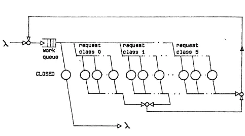
The model for the transport protocol of the OSI is now presented. Consider a

TSDC of an arbitrary request class. It progresses through a series of service phases starting with a request for its transport connection and ends with the termination

of its transport connection, the

CLOSED

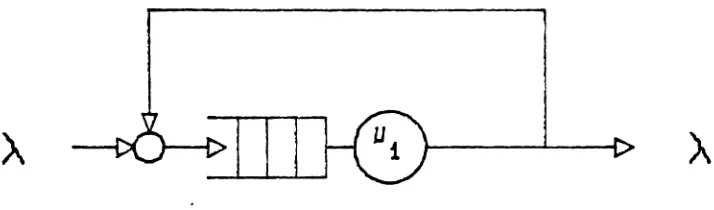
phase (see Figure 3).

Some of the service phases require only the services of the local transport

entity. The rest must use both the transport entity and external services Irorn the

network layer and the peer transport entity. The model for such a service phase is

CLOSED

Figure 3:

General Madel far TSOU

Service

Figure 4:

Model for a Phase with only Local Service

l'qua

I.

as the fIrsL ph~se 0

r

Sf'r v1(' t' 1s tIH' 11sCr s r(:' q1j('St. w

It

i('h rl'qUIres 0IIIY thl' entity's services. The last phase is the C~LOSEDphase which does not feedback. If

this model (combined with the assumption that the actual transport entity times

are almost negligible) was all there was to the analytic model, a solution would

already be available. Kleinrock has this model, the processor sharing model [10],

for the ~I/G/1 case solved for both the average response time, T(x), for a customer

requiring x seconds of processing time

i:

where

T(x)

=

1-p

(4.14)

p

==

utilization

and the waiting time.

\\r(x).

for that customer.

W(x)=~

I-p

(4.1.5)

Some external servicing occurs in the full model (Figure 3). The external

server is comprised of a network service and the service of a peer transport entity.

If the service times of the messages are strictly exponential with no priority

struc-ture or local balance for the model held for all classes of customers, the ~orton

theorem method could be applicable. But in the

NBS

implementation of this

pro-tocol, the DR TPDU is given top priority. Furthermore, service times are not

strictly exponential. Now, if the transmission phase alone is considered and no

timeouts occur, then the required exponential service time exists. The timeout

res-tr iction could be lifted by having randomly occurring tirneouts as shown by Reiser

distr ibutions. In la ct , thrr«- or the -ix cla~sf-'s

or

'I'~[)l'~ Jo not h:l\'C' any expOll(:'fl-tially distributed service times. They are all non-zero mean uniform distribut.ions.

Because the protocol is operating in wide area networks, the network times

are significantly greater than the transport entity times. As long as these network

times are independent of the transport entity. and as long as the network times

remain exponential, then the input stream, due to the external server, remains

Markovian. But if the network is congested or has an unacceptable error rate.

then timeouts and lost acknowledgements make arrivals to the transport entity

dependent on the network time. Appendix D has a list of the four network types

for which a HC").,[P network solution would exist. Sinre this protocol gives the DR

TPDl~ priority, an exact BC'\·lP solution does not exist, suggesting a need for an

alternate solution. This alternate method is to assume a product form solution

and to find out when the DR priority interferes with that assumption.

Each class of message in Figure 3 uses the local transport entity and

some-tirnes uses external service. The model of the

ESTiill

class TSDL~. Figure .5,

illus-trates this point.

Here the connection establishment (CON

EST),

data transfer (D~..\.T~~

XFER).

and connection termination (CON TER.NI) phases are the only service phases to

use both the local transport entity and the external server. The other service

phases use only the local transport entity. These phases are the user interface

(CSER). network connection (:\ET CON), data transfer request (DATA XFER).

extsrnal

server'

n

e

"t

Figure 5:

BC~P

Medel of SOLID ESTAB

Class TSDU

connection t.er rniuation ((.LOSI~I)).

Note also from Figure.5. that the state of the system can be described as the

number of TSDUs in the transport entity, nt ' and the number of TSDUs in

exter-nal service, n_{e •}

With the

BCwlP

assumption, the time to serve a

TSD(->",

T. is expressed as the

sum of t\VO other times: the time taken in the local transport entity,

T,

and the

time taken in external service. T_{e .} That is

T

So

T

(4.16)

(-1.L7)

The functional summary diagram of the SOLID_ESTA.B class model in Figure 6 shows the reduction to two functional nodes.

4.2.2.1. The Processor Sharing Node

From the model, onecan see that

x

where

the required service time

x

-- for a TSDU

and

f..Ll

0(0

(!j)

0(2

~

to

_(S)

work

queue

f

0

f

0

0

Olt

_external

server

Figure 6: General Model of the Tran9port Portocol

~i[lce the arrival rate. A, IS very small, and the servi.:e tinu- of rhe eu t.ity IS

J-LL also very small, the utilization of the transport entity, PI' is negligible. So,

(4.19) As a digression, consider this node to be an Nl/M/l node. The same result would be reached for

T

_{t .}

T.\JA/I

PI

*1-1 - PI A

1

CtlJ..11

=

1 - PI

1

number of services (4.20)

Thus, the time taken in the transport entity is approximately the number of

services required. The units llsed is the time taken for the kernel resident

tran-sport entity to process a request. In this dissertation, one millisecond is arbitrarily

chosen as this reference unit of time.

4.2.2.2. The External Node

Because theexternal node is modeled as an 1\;[j

G

j'XJ server,

(4.~1)

39

CH~L\PTER 5

TL\1E DELi\.Y ANALYSIS

This dissertation analyzes the mean, end-to-end time delay of the transport protocol. The tools for the analysis of time delay are obtained by making use of distributions for service phase success, TSDU size, and window size. The service phase success probabilities are developed first.

The local entity and the external server are treated separately. Therefore, the mean value for the entity time is given by finding the mean number of services a class of TSDl~ receives. The external service time is more difficult to obtain.

The discussion of external service time is broken up into two sections: one sec-tion discusses the time taken for overhead phases, those not directly involved in data transfer, and the other section addresses data transmission. In the data transmission section, virtual circuit transmission and datagram transmission are treated separately.

5.1. Probability that a. Service Phase Does Not Timeout

The probability that a given external phase of service does not timeout. Ph ,IS

40

rrhat is

Pii = P[TTPDU

+

T

ND

+

T

e o R

+

T

ND

<

timer]

where

TTPDU

==

time to transmit the TPDU.

T

eOR

==

time to transmit the corresponding TPDC

Let

(5.1)

~Y = TTPDU

+

T ND

+

TeoR

+

T;vD

Furthermore, let each of the random variables contributing to

X

be independent random variables. Then it is found that

and

a./~

=

a

}PDU

+

2

*

a

~D

+

fI

~OR

In order to find the probability that a data phase is successful, the distribu-tion for the time taken during the data transmission phase is needed. From that distribution, the probability of a successful data transmission is determined. Let

--'Y_i be the amount of time required to send packet i and receive its acknowledge-ment.

It

is easily seen that the event

[packet times out]

==

(Xi?

timeout)

(.5.2)

A window is made up of Xtsdu packets, so within a window, a timeout occurs if

This event IS difficult to quantify, but the complement ot' that event IS readily

obtained.

[packet doesn't timeout]

==

n

("Yl

s; timeout

l

aU i ,

,

P[packet doesn't t£meout] =

i~l

(XI

::S t£meout)

where ~ =: min(Itsdu' no. of packets in the message).

The mean value of

..iY

_i is

:\0\\

2 ? ') .} ?

a ..

r.

= fIjVD

+

aF.fD

+

fIACK

+

IT

Dr

for

4¥t ,

i = 1,2...Xtsdu, assuming TACK, T_{D r ,} and T_ND are independent. Approximate

Xi

as a normal random variable

and then P[timeout] is written as

[

4¥i -

Xi

rir ans -

~¥i

I

P(timeout]

=

P

>

ax,

ax,

=

p

[z

>

_rt_ra_n_S_-_4'¥_i

I

ax,

(.5.-1 )

(S.5)

(S.6)

(.5.7)

(5.8)

(5.9)

Hence ,

Pt« =

P [no timeout in the uJ£ndow]

( )

u,«;

= 1 --

P[tilneout]

(5.10)

For the other phases, the probability that a phase does not timeout is found by assuming the external time is a normally distributed ra ndom variable ..

t'".

This random variable is then compared with the timer value to determine the probabil-ity of success. Probabilities for the overhead phases requiring external service fol-low.

Connection Establishment:

and

Pte

=

p[~y ~

initiate]

where

initiate

==

the connection timer value.

Connection Termination:

x

=

T

DR

+

T

ND

+

T

DC

+ T

iVD

Ptd = P[~Y~terminate]

where

terminate

==

the termination timer value.

Short Transfers:

Ptxs =

P

[.¥::;

initiate]

(.5.11)

(5.12)

(5.13) (5.14 )

(5.t5 )

(,5.16)

where the expected value of a CR TPDlf during short transfers is used instead of

5.2. Probability the External Ser-vice Phase is successful

The probability of service phase i succeeding, Pi, deals with external service

phases. It is the probability that a TPDlJ is successfully sent and acknowledged by the appropriate TPDlT within a specific timeout value and is not lost in the net-work layer. Thus.

[

T PD [ rexchange does not take too lOng]

p£

=

P .4.JVD

TPDC"s are not lost

It is useful to define the following terms:

(1)

PSi

=

phase i is successful.

(2) PC"z

=

phase i is not successful.

(3) TO:,

==

Phase i, in a error free network, exceeds the time allotted to it specified by the timer value.

(4)

L,

==

a TDPU active during phase i is lost.

(5) Ph

==

P{ The time taken to execute a service phase does not exceed the timer

value} ,

Pti

+

qti = 1.

It is apparent that

qti =

P [ TO

I ] .

(6)

q

=

P[L

i ]

for all

i

and

P

+

q=l.

It is interesting to note that if either event

TO

l or £1 occurs. a timeout occurs.

However, these are two different events which contribute to the issuance of a

P [ P

c, ]

= P [ ( TO lOR LI

Jl

=

qtl

+

q -

P [

(TOi AND

Ld ]

Now the actual time taken to send a TPDU through the network is indepen-dent of the loss probability because the loss mechanism works on TPDlJs with equal malice.

It

does not differentiate between tardy TPDl~sand swift

TPDl;s. So

= qti * P

+

q

and

Pi

=

1 -

p[PU

_{i ]}

=

Ptl *P

where

=

C,d,IS,X

5.2.1.1. Expected Number of Service Phases

(5.19)

The expected number of service phases for the transport entity approximates

T

_{t •} It is made up of two types of values. One type is services involving only the local transport entity. The second type of value involves service phases that send the TSDU for external service. Let

V£

be the number of times a

TSDU

visits the transport entity in phasei. When only local service in phase i is required. Vi 1 .

When external service IS required, Vi can assume one of two values. 1

Pi

if

retransmissions are unlimited, and

~

Pi

f +1

-q--,

if

retransmissions are limited to f.

P1

In these two expressions, P, is the P[phase

qi - P [phase i fails]

=

1- Pi

-15

Let the first of the t\VO values of the random variable, ~/l' be the geomet.r ic value. Let the second value, be the truncated geometric value which is developed in

Appendix A. Because retransmissions are actually limited by the protocol, the

truncated geometric value, _1_

Pi

Transport Entity Time

ql+1 .

- - , IS used. In summary,

Pi

last ~hase

= ~ Vi

i=l

where

r _

r

1 for phases requiring only local service

Vi -

l-q!~l

I

I for phases requiring external service

Pi

For phases requiring external service, the difference between the geometric and

ql+1

truncated geometric value is only _ 1- . Because Pi

>

0.5 for a good

implementa-Pi

tion, the geometric value provides an excellent approximation.

5.3. External Service Time

5.3.1. Introduction

In the study of external service time, two simplifying assumptions are made.

They deal with network error and random variable treatment.

Network error is treated in the following \vay. Loss probabilities are assigned

to transactions. It is these probabilities which are used and not the bit error rate

Any

given phase has one or more 1'PDlfs associated

with

it. The t ime taken

to complete a phase is usually the sum of several random variables. Because the

exact treatment of the resultant random variable is extremely cumbersome, the

following approximation is used. If the resultant random variable is dominated by

a few random variables. the small components are either ignored or treated as

con-stants.

It is shown in Appendix B that

T

_e is the sum of the times the TSDU spends in

each phase of external service. This result has a very nice intuitive appeal: The

external service time is found by simply summing the time spent in each phase of

service.

The external time is made up of the time to send data, which is the purpose of

the protocol. It is also made up of overhead phases which ensure orderly data

transfer. The next section covers the mean external service time for overhead

phases. This is followed by a derivation of the external service time for data

transmission.

5.3.2. Overhead TPDU Phases

To accomplish reliable end-to-end data transfer, some overhead is inherent.

The TPDUs used in these phases are not segmented any further by the protocol.

·-(7

T\NO expressions are now developed La examine the time taken in a phase: the time taken to complete a phase of service when the nurnber of retransmissions are unlimited and

the time taken

to

complete

a

phase

of service when

the number

of

retransmissions are limited.

5.3.2.1. Unlimited Retransmission Assumption

First, recall that Pz = P[TPDU succeeds] and Pi

+

qt==1 . If there is no limit to the number

of

retransmissions, the expected time to complete

a

given service phase iseasy to derive. Let the following values be defined:

E [ T_{e ]}

-=

E[Time to complete a service phase]

T

TPDU

==

E[Time to transmit a

TPDlT]

T

COR

==

E[Time

to

transmit the corresponding

TPDU]

TO

==

Timeout value

T

_1VD

==

E[Network

delay]

TTC

==

TTPDU

+

T

e o R ·

Now

E[T

_e] = E[Time to complete a phase

I

successful attempt]p

+

E [Time to complete a phase

I

unsuccessful attempt]ql

=

(TTPDU

+

T

_ND

+

T

e o R

+

TtVD)Pi

+

(TO

+

Te)qi

= TTC

+

q_<>,

t

_YD

+

~

1"'0

Pl

·18

(.1.21 )

As Pi vanishes,

T

_e becomes very large. However, an unbounded service time

is unsatisfactory. To prevent this, the protocol has a fixed number of

retransmis-sions. The last retransmission is special, however.

If

the previous transmission

attempts fail, the timer value is set to accommodate the longest anticipated delay

to maximize a reasonable chance of success. The external service time of the fixed

retransmission strategy is now examined.

5.3.2.2. Limited Retransmission Assumption

In an actual protocol, the number of retransmissions is limited to a number,

f .

For the moment let

tx=

TTPDU

+

2T

ND

+

Teo»

and

ei

==

time taken after i attempts

The expected time to complete an overhead service phase then becomes

where

E

[en]

=

tz

*

Pi

+

(TO

+

E

[en-i-l ])

*

qi

for

n=1,2, ...

.t.i

and

(5.23)

(5.24)

(5.26)

where PI is the probability that the last attempt is successful. which is very close

1""his Ior wa.rd recursion is now oxarnined . Let

ao

==

E [ T

e

J

az

==

E

[e

i ]

From Equation 5.25.

which can be rearranged to

.9

(5.27)

(5.28)

(5.29)

Let ..-l

and

....L

and

B -

-

J:L

Equation .5.29 becomes

qz qz

(5.30)

(5.31 ) This recursion takes the form

n - l

an

=

.It nao

+

B

I ..

4.k

k=O

To prove this, examine the inductivestep:

(5.32)

(

n-l]

=

it. ..4

n

ao

+

B

I

~4k

k=O

+B

n-L

= An-to1 a0

+

B

2

.4k~1

+

B

50

n

4-1 nr Lao

+

B~ ~-ik

k-=O

Equation 5.32 is used to determine af.

f -1

t f

+

B

>.

J.,tk

af

=

./t ao - . J '"1.

k=O

Because

ao

=

E [T

e ].

E [

t; ]

is found by solving equation .5.33 for

ao·

(5.3:3 )

[r

f -1 1

at -

B~

-E[T

e ]

k~O qi

=

ao

=

[:i

r

1

- [:1

r

q/

at -

B

q/

(,5.34)

Pz qi

The forward recursion leads to

Since the last, or

f

th, transmission is governed by the give_up timer whieh is large

enough to virtually ensure a successful transmission, PI-1. Equation ,5.34 becomes

E [ Te ] = tx

+

TO ;:

(1 -

q! )

CS.35)

This is the expectation for the time taken in any phase of service which is not

directly involved in the transmission of data.

5.3.3. Service Time for' the Data Transmission Phases

Another model is used to aid in the analysis of data transmission. This model,

a (n)

I

i

I

A.

I

!

I

r---, I

_~_~--.---l

b (n)

--_._._-{:.>

51

where a (n)

=

P[ TSDU

arriving has n packets]

b

(n)

=

P[ TSDU entering data transmission service has n packets]

52

model, the expected time to t.ransrnit data can be developed.

The service time for the data transmission phases must take both virtual

cir-cuit and datagram transmissions into account. In both cases an assumption

grant-ing unlimited retransmission is given first as the solution is very straightforward.

This is followed by the more realistic restriction on retransmissions.

Although there is a difference between datagram service and virtual circuit service, the development is roughly the same. So the service time is given first and the special considerations given to datagram service are then discussed.

5.3.3.1. Unlimited Retransmission Assumption

When the number of retransmissions is unlimited and the probability of sue-cess IS constant, the probability of retransmission becomes geometrically

distri-buted. This assumption yields the quickest result for the service time.

[ ] _[ - - - dmax

1

(

-E T

e =Px

2

T

1VD

+

TACK+A +qx.rtrans+

T

e ' )

net_cap

where

:c

A

=

2:

na(n) n=O

and

T

e ' = E[Tirne to transmit data after a timeout has occured]

[ T

-

-

dmax]

(

-=

Pz 2 .VD

+

TACK

+

B

+

qx rir ans

+

T_{e ' )}

net_cap

Hence,

f/J

+ -

rlr ans

P.l

Now with A geometrically distributed, B is also geometrically distributed. This results in

r;

=

2T,VD

+

TACK

+

~4_d_m_a_x_

+

_q_xrtrans

net_cap PI

Combining Equations .5.36 and 5.39

E [T]

_e

₌

."') T-

_{~ .VD}

+

T-

_ACK

+

A-

dmax

+

~

rirans

_co

net_cap PI

Using Equations .5.36and 5.38, E [

r, ]

can be written as

(,5.39)

(5.40)

= 2TiVD

+

TACK+PI

*

dmax

(if -

B)

net_cap

(,5.41)

+

dmax

B

+

~

rtrans

net_cap Px

which allows a tabulation of

E [

r, ]

even if A is not geometrically distributed. But

as Pi gets smaller, this result becomes a very poor prediction of time delay.

5.3.3.2. Limited Retransmissions

Consider a limited amount of retransmissions. This gives rise to a truncated geometric distribution.

54

II = 2T_VD

+

TACK

+

B

dma.r

net_cap

Then

E[e

n ]

=

ix

"* Px

+

(TtTans

+

E[en+t])

qx for n=1,2,:3 ....

!

-1 (.').44)

and

Let

and

Equation ,5.45 becomes

andso

This becomes

E [ef ] = tx

~

Pf - tx

~ = tr

*

Px

+

rtrans

*

qx

(.5.4.5)

(.5.46)

So

but

(5.47)