Improvement of Mining Fuzzy Multiple Level Association Rules from Quantitative Data

Improvement of Mining Fuzzy Multiple-Level Association

Rules from Quantitative Data

Alireza Mirzaei Nejad Kousari1, Seyed Javad Mirabedini2, Ehsan Ghasemkhani1

1

Department of Computer Science, East Tehran (Ghiamdasht) Branch, Islamic Azad University, Tehran, Iran; 2Department of Com-puter Science, Central Tehran Branch, Islamic Azad University, Tehran, Iran.

Email: {ali_mnkt, jvd2205}@yahoo.com, [email protected]

Received November 30th, 2011; revised December 31st, 2011; accepted January 11th, 2012

ABSTRACT

Data-mining techniques have been developed to turn data into useful task-oriented knowledge. Most algorithms for mining association rules identify relationships among transactions using binary values and find rules at a single-concept level. Extracting multilevel association rules in transaction databases is most commonly used in data mining. This paper proposes a multilevel fuzzy association rule mining model for extraction of implicit knowledge which stored as quanti- tative values in transactions. For this reason it uses different support value at each level as well as different membership function for each item. By integrating fuzzy-set concepts, data-mining technologies and multiple-level taxonomy, our method finds fuzzy association rules from transaction data sets. This approach adopts a top-down progressively deep- ening approach to derive large itemsets and also incorporates fuzzy boundaries instead of sharp boundary intervals. Comparing our method with previous ones in simulation shows that the proposed method maintains higher precision, the mined rules are closer to reality, and it gives ability to mine association rules at different levels based on the user’s tendency as well.

Keywords: Association Rule; Data Mining; Fuzzy Set; Quantitative Value; Taxonomy

1. Introduction

A useful technique which turns data into task-oriented knowledge is known as data-mining. The mining appro- aches, found from the classes where the information is issued, may be classified as finding association rules, classification rules, clustering rules and sequential rules and etc. An Association rule mining is an important pro- cess in data mining, which determines the correlation be- tween items belonging to a transaction database [1-3]. Association rules are extensively carried out and are use- ful for planning and marketing. For example, they can be used to inform supermarket officials of what products the customers have a tendency to buy together, like “if cus- tomers buy milk, they are more likely to buy bread as well “which can be mined out. The supermarket mana- ger then knows to place the milk and bread in the same place in the store to tempt the customers to buy them simultaneously. In general, every association rule must satisfy two user specified constraints: support and confi-dence. The support of a rule X Y is defined as the fraction of transactions that contain



XY, where X and Y are disjoint sets of items from the given database [4,5]. The confidence is defined as the ratio support (XY)/support(X). Here the aim is to find all rules that

Satisfy user specified minimum support and confidence values. Many algorithms for mining association rules from transactions were proposed, most of which were based upon the Apriori algorithm where it generated and tested candidate itemsets step by step. However, this pro- cessing way might cause high computational costs and iterative database scans. In the past, research has focused on showing binary-valued transaction data. Transaction data usually consists of quantitative values, which then can be dealt with by designing a data-mining algorithm, but this has proved to be a challenge to researches in this field. The majority of algorithms used for association rule mining are to association rules on the single- concept level. Nonetheless using mining multiple-concept- level rules may result in the finding of more exact and useful information from the data. Relevant data item taxono-mies are normally preconceived and can be symbolized using hierarchy trees. Mining multi-level association rules are driven by several reasons, such as:

 The multi-level association rules are more under- standable and are more interpretable for users.

 The multi-level association rules can give us solutions for the unnecessary and unwanted rules.

concept hierarchies are copied by a directed acyclic graph (DAG). A concept hierarchy symbolizes the rela- tionships of the generality and requirement between the items, and classifies them at several stages of abstraction. These concept hierarchies are available, or formed by ex- perts in the field of application. For example, a user may not only be concerned with the associations between “computer” and “printer”, but also wants to know the association between desktop PC price and laser printer price.

Another trend to deal with the problem is based on fuzzy theory [6] which provides an excellent means to model the “fuzzy” boundaries of linguistic terms by in- troducing gradual membership [7]. This paper proposes a fuzzy multiple-level mining algorithm for extracting im- plicit knowledge from transactions stored as quantitative values. Frequent itemsets can be found from proposed algorithm which takes up a top-down progressively by deepening approach. It integrates fuzzy-set concepts data- mining technologies and multiple-level taxonomy to find fuzzy association rules from a transaction data sets. The mined rules are more natural and understandable for hu- man beings. Fuzzy sets have been used for many applica- tions and resulted in good effects. Fuzzy set theory is used more often in intelligent systems; the reason using it is because is simple and similar to human reasoning. Several fuzzy learning algorithms is designed and used for good effect in specific knowledge for generating rules from a sets of data which is given.

2. Apriori Algorithm and Apriori Property

Now we know that to find frequent itemsets, it is effec-tive to use Apriori algorithm. Apriori employs an itera-tive approach known as level-wise search, where k- itemsets are used to explore k + 1-itemsets. Apriori, exploits the following property: If an itemset is frequent, so are all its subsets [8]. The idea is frequent itemset must have subsets of frequent itemsets. Frequent itemsets can be made of mixture of smaller frequent itemsets one after another. Let k-itemset express an itemset having k items. Let Lk represent the set of frequent k-itemsets and

Ck the set of candidate k-itemsets. Therefore the

algo-rithm to generate the frequent itemsets is follows: A1) Ck is generated by joining the itemsets in Lk–1 A2) The itemsets in Ck which have some (k – 1)-subset

that is not in Lk–1 are deleted.

A3) The support of itemsets in Ck is calculated through

data base scan to decide Lk.

After L1 chosen first through data base scan, all three A1-A3 procedures are iterated until Lk becomes empty

set. The association rules are extracted by combining the decided frequent itemsets to calculate the confidence of the association rule [9].

3. Multilevel Association Concept

Mining association rules at multiple concept levels may, however, lead to discovery of more general and impor- tant knowledge from data. Relevant item taxonomies are usually predefined in real‐world applications and can be represented as hierarchy trees. Terminal nodes on the trees represent actual items appearing in transactions; in- ternal nodes represent classes or concepts formed from lower‐level [10].

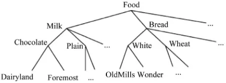
In Figure 1, the root node is at level 0, the internal

nodes representing categories (such as “milk”) are at level 1, the internal nodes representing flavors (such as “chocolate”) are at level 2, and the terminal nodes repre-senting brands (such as “Foremost”) are at level 3. Only terminal nodes appear in transactions [3]. In predefined taxonomies are first encoded using sequences of numbers and the symbol “*” according to their positions in the hierarchy tree. For example, the internal node “Milk” in

Figure 1 would be represented by 1**, the internal node

“Chocolate” by 11*, and the terminal node “Dairyland” by 111 [3].

4. The Proposed Model

In this part we present our algorithm which is called im- proved fuzzy mining algorithm using taxonomy (IFMAT) which is modified the version of previous fuzzy mining algorithm presented in [3]. It consist of data mining, multi-level taxonomy and a set of membership functions to explore fuzzy association rules in accordance a given transaction dataset.

Details of IFMAT algorithm are as following:

Step-1

Use a sequence of numbers and the symbol “*” to en-code the predefined taxonomy by using the formula

*10

C i

where is the location number of node at current level (a set of contiguous integers starting from 1 is assigned to the nodes from left to right as location number), C denotes the code for the th node at current level and

i

i 

is the code of parent of the ith node at current level. An example of a hierarchy and the code for each node are shown in Figure 2, Then After the coding, each item recorded in a customer transaction database will be

Figure 2. An example of a hierarchy with node code.

represented by its code.





1 max k maxhkj k

j l j

count  Count

  _l

then set k = 1, r = 1 where k, is the current level number,

1 k x

x is the number of level in a given tax-onomy and r is to represent the number of items stored in the current frequent itemsets.

set MaxRkj as the region with Max

k j

count

 for

item Ikj . If the value Max

k j

count

 of a region MaxRkj is equal or greater than minimum support

value () in the current level, place Max k j

count

 , into the frequent 1. itemset ( 1) .

k

L

Step-2

In each transaction datum Di where Di is the i-th tran- saction, (n is the number of transaction), add all of the items with the identical first

1 i n

K digit, compute the addition of each groups in the transaction and elimi- nate the groups which their addition are less than  where  is the predefined minimum support value in the current level.

Step-6

If 1 is null, then increase by one,

k

L K r1 and go

to step 2 otherwise set r r 1 and go to the next step.

Step-7

The procedures below are carried out for different value of r:

Step-3 _{a) If} r2 produce the candidate set 2, where

is the set of candidate itemset with 2 items on level from 1 1 to explore “level-crossing” of fre- quent itemset. Candidate itemsets on certain levels may thus contain other-level items. For example, candidate 2- itemsets on level 2 are not limited to containing only pairs of frequent items on level 2. Instead, frequent items on level 2 may be paired with frequent items on level 1 to form candidate 2-itemsets on level 2 (such as {11*, 2**}) [11,12]. Each 2-itemset in ₂ must include at least one item in the 1 and the next item should not be its ancestor in the taxonomy [3]. All possible 2-itemsets are collected in .

k C 2 k C k 1 2

1, 1, L L L

2

r

3_{, ,} k

L  k C k C k L

We considered different membership function for dif- ferent data items. for that each data item has its own cha- racteristics and its own membership function, then con- vert the value of each transaction datum Di for each encoded group name

k ij

V

k j

I into a fuzzy set shown as a following by mapping on the specified membership function, where

k ijl f k ij V k j

I is the j-th item on level , is the quantitative value of

k V_ijk Ik_j in Di,

k j

h is the

k k k

j

I , Rjl (1 l hj) is the

number of fuzzy regions for -th

l fuzzy region of k j

I , is s fuzzy member- ship value in , .

k ijl f k ij V k il

R 1 l h

2

b) If _{, Generate the candidate set} , where is the set of candidate itemset with -items on level from 1

k r C k r C k r k r

L in a way similar to that in the

algorithm [1].

apriori

1 2

1 2

k k k

ij ij ijh

k k k

j j jh

f f f

R R R

            Step-4

Compute the value of each fuzzy region in the transaction data as following, where is the sum-

k il R k il Count Step-8

For each obtained candidate r-itemset S with items





k r

C

mation of fijlk:

1 n k k il ijl i Count f  



a) Compute the fuzzy value of in each transaction datum using the minimum operator as a follow :

S

i

D Step-5





min , , ,

r

is is is is

f  f f  f

Specify Maxcountkj k

using the following formula where Maxcountj is the maximum count value

among Countjl values (1 k j

l h

1

n

s is

i

Count f







c) Providing that Counts is not less than minimum

support  in the current level, insert S in Lk_r Step-9

If equal null then increase K by one and go to the next step otherwise increase r by one and go to step 7.

k r

L

Step-10

If KX then go to step 11, where X is The num-ber of levels in a given taxonomy. otherwise set r1 and go to step 2 .

Step-11

make the fuzzy association rules for all frequent r- itemset including S 





and A B , A B S

 Compute the confidence value of all association rules by:

 

 

1

1 min Confidence

min

n

is i

n

iA i

f

f 

 





Step-12

Select the rules which have confidence values not less than predefined confidence threshold , where  is the predefined minimum confidence value.

5. An Example

Please see the following example in order to have a bet- ter understanding of the algorithm:

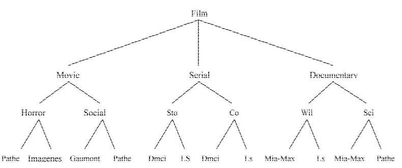
In this example, we use six transactions related to the film sales in a video shop as shown in Table 1 and we use a predefined taxonomy as shown in Figure 3.

As it is shown in Figure 3, we divide the films into three classes of movies, serials and documentaries. Each of these classes have got subordinates, specifying the type of film and the producing companies. For each class of the films, we consider a unique membership function and for each of the membership functions, we consider three fuzzy regions called low, middle and high regions. The membership function related to the serials has been shown in Figure 4 and the membership function for documentary movies has been shown in Figure 5 and the membership function for movies has been shown in Fig- ure 6.

Details of the proposed mining algorithm are given below.

Step 1:

First we change each of the nodes of the taxonomy shown in Figure 3 into their coded equivalents, and the result has been shown in Figure 2. Then we change each of the members of the transactions to their coded equiva- lents, according to Figure 2, the result of which has been.

Table 1. Six example transactions.

Items TID

(Pathe horror movie, 1) (Imagenes horror movie, 4) (Dmci story serial, 4) (LS story serial, 6) (Mia-Max wild life documentary, 7)

D1

(Pathe horror movie, 3) (Imagenes horror movie, 3) (Gaumont social movie, 1) (Dmci comic serial, 5) (LS comic serial, 3) (Pathe scientific documentary, 4) (Mia-Max scientific documentary, 4)

D2

(Dmci story serial, 7) (Dmci comic serial, 8) (LS wild life documentary, 5) (Pathe scientific documentary, 7) D3

(Pathe horror movie, 2) (Dmci story serial, 5) (LS wild life documentary, 5) D4

(Dmci story serial, 5) (LS comic serial, 4) D5

(Pathe horror movie, 3) (Imagenes horror movie, 10) D6

Figure 4. The membership functions used for number of serials sales.

Figure 5. The membership functions used for number of documentary sales.

Figure 6. The membership functions used for number of movie sales.

shown in Table 2.

We then consider a variable called and a variable called and give them a value of one; where stores in itself the number of taxonomy levels and shows the number of items existing in current frequent itemset.

k

r k

r

Step 2:

We place all items in which the of their first digit is similar in a transaction in one single group and sum up their values. For example we classify the items (111,1) (112,4) in Group (1**,5). The result of this task has been shown for all transactions in Table 3.

k

Step 3:

We change the groups obtained in the previous step into the fuzzy set of equation based on the membership function. For example, let’s consider the Group (1**, 5).

Table 2. Encoded transaction data in the example.

TID Items D1 (111,1) (112,4) (211,4) (212,6) (311,7)

D2 (111,3) (112,3) (121,1) (221,5) (222,3) (322,4) (321,4)

D3 (211,7) (221,8) (312,5) (322,7)

D4 (111,2) (211,5) (312,5)

D5 (211,5) (222,4)

D6 (111,3) (112,10) (411,3) (412,9)

Table 3. Level-1 representation in the example.

TID Items D1 (1**,5) (2**,10) (311,7)

D2 (1**,7) (2**,8) (3**,8)

D3 (2**,15) (3**,12)

D4 (1**,2) (2**,5) (3**,5)

D5 (2**,9)

D6 (1**,13)

Since according to the predefined taxonomy in Figure 3, this Group is related to the movies, so we use the mem- bership function related to the sales of the movies. The value 5 in the membership function related to the sale of movies is equal to 0.2 for low region, 0.8 for middle re-gion and 0 for high rere-gion. The equal fuzzy set for all items of the transactions have been shown in Table 4.

Step 4:

We calculate the sum of values in each fuzzy region in all transactions. Let’s consider the as an ex- ample. The sum of fuzzy values of this region in all tran- sactions is obtained through the equation 0 + 0 + 0.8 + 0 + 0 + 0.2 = 1. The sum of fuzzy values for each individ-ual region has been shown in Table 5.

1**.Low

Step 5:

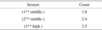
Considering the previous step, the fuzzy region is se-lected with the highest value for each group. As an ex-ample, let’s consider the Group . Its value for Low region is equal to 1 (one), for middle region is equal to 1.8 and for high region is equal to 1.2.

1**

Since the value of middle region, i.e. 1.8 is higher than the other two regions, the middle fuzzy region is chosen as the representative of Group for other processes. This task is also carried out for other groups. Each of these values is compared with the minimum support de-fined in level kth, and in case it is bigger or equal with the predefined minimum support in level kth, it is added to at that level. For instance, let’s assume the minimum support at the first level is considered as 1.8, so since the

values of 1* , and ,

are bigger or equal to 1.8, taking into account the values obtained from Table 5, this single-member sets are placed in according to the Table 6. Since is not

1**

Middle 1

1

L

*.Middle

1 1

L

2 **. 3**.Middle

1 1

Table 4. The level-1 fuzzy sets transformed from the data in Table 3.

TID Level-1 fuzzy set

D1 0.2 0.8 1**.low 1**.middle  _      0.4 0.6 + 2**.middle 2**.high       1 3**.high       D2 0.8 0.2 + 1**.middle 1**.high       0.8 0.2 + 2**.middle 2**.high       1 3**.high       D3 1 2**.high       1 3**.high       D4 0.8 0.2 + 1**.low 1**.high       0.4 0.6 + 2**.low 2**.middle       0.5 0.5 + 3**.middle 3**.high       D5 0.6 0.4 + 2**.middle 2**.high       D6 1 1**.high      

Table 5. The counts of the level-1 fuzzy regions.

count Items 1 (1**.low) 1.8 (1**.middle ) 1.2 (1**.high ) 0.4 (2**.low) 2.4 (2**.middle) 2.2 (2**.high) 0 (3**.high) 0.5 (3**.high) 3.5 (3**.high)

Table 6. The set of frequent 1-itemsets for level one.

Itemset Count (1**.middle ) 1.8 (2**.middle ) 2.4 (3**.high ) 3.5

equal to null, we can then go to the next step.

Step 6:

The candidate set is generated from and here since consists of 3 members of ,

and , members of has been shown in Table 7.

1 2 C **. 1 1 L 1** 1 1 L Midd .Middle 1 2 C

2 **. le 3 Middle

Steps 7, 8, 9 and 10:

The following steps are carried out for the two-mem- ber items in C12:

a) The fuzzy membership value of each of the two- member sets inside the is calculated based on the predefined membership function for each individual item, for the whole transactions. For example, consider the two-member set as an example.

1 2

C

ddl





Table 7. The counts of the level-1 fuzzy regions.

Itemset (1**.middle , 2**.middle)

(1**.middle , 3**.high) (2**.middle , 3**.high)

The fuzzy membership value of this set for transaction 1 is calculated as: min (0.8, 1) = 0.8. This operation must be carried out for all transactions, the final result of which has been shown in Table 8.

D

b) The sum of fuzzy membership values obtained in Section A for each individual two-membership sets are calculated in . The final result has been shown in

Table 9.

1 2

C

c) Since in the sets obtained, only the value of the set





1 2

L

is bigger and/or equal to the value of predefined minimum support in the first level, so the is only equal to one member. All frequent itemsets in Level 1 have been shown in Table 10.

We consider the variable r equal to 2, where r repre-sents the number of the members of those sets that are within the current itemset. Since is only equal to a 2-member set, and we can not produce 3-member sets at Level 2, so we add one unit to and go to the Step 2. The final result for the frequent itemset for Level 2, and for Level 3 with minsupp = 2, have been shown in

Ta-bles 11 and 12, respectively. Since there is no Level 4,

we go to the next step .

1 2

L

k

Step 11:

We will find the fuzzy association rules based on the frequent itemset obtained from the previous steps:  We discover all probable rules from the frequent

Table 8. The membership values for 1**.Middle, 3** high.

Min(1**.middle , 3**.high) 3**.high

1**.middle TID

0.8 1

0.8 D1

0.8 1

0.8 D2

0 1

0 D3

0.2 0.5

0.2 D4

0 0

0 D5

0 0

0 D6

Table 9. The counts of the 2-itemsets at level 1.

Count Itemset

1.4 (1**.middle, 2**.middle)

1.8 (1**.middle, 3**.high)

1.7 (2**.middle, 3**.high)

Table 10. All frequent itemsets in level.

Itemset

Count (1**.middle )

1.8

(2**.middle )

2.4 (3**.high )

3.5 (1**.middle, 3**.high)

1.8

Table 11. The set of level-2 frequent itemsets.

Itemset

Count (11*.middle )

2

(21*.middle )

2.6 (31*.high )

2 (22*.middle) 2 (32*.high ) 2 (11*.middle, 3**.high) 2

Table 12. The set of level-3 frequent itemsets.

Itemset Count (111.low ) 3 (211.middle ) 2.6 (111.middle, 3**.high) 2.1

sociation rules, can be extracted from the frequent itemset with minimum two members.

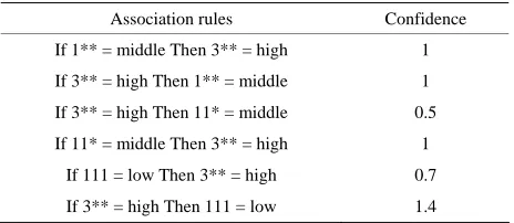
If 1** = middle Then 3** = high If 3** = high Then 1** = middle If 3** = high Then 11* = middle If 11* = middle Then 3** = high If 111 = low Then 3** = high If 3** = high Then 111 = low

 For the rules achieved, we must find the confidence value of each rule. For example, let’s consider the

following rule:

If 1** = middle Then 3** = high

The confidence value for this rule is obtained as fol-lows:

We find the confidence value for the individual rules. The confidence value for all rules has been shown in

Table 13.

Step 12:

The confidence value of all rules are studied with pre- defined minimum confidence threshold and the rules, whose confidence value is bigger than or equal to the predefined minimum confidence threshold, are chosen as final rules. For example, if the minimum confidence value is equal to 1, the final rules shall be as follows:

If 1** = middle Then 3** = high IF 3** = high Then 1** = middle If 11* = middle Then 3** = high If 3** = high Then 111 = low

6. Experimental Results

In this part, we will analyze the results of the experi- ments and analyses made. The proposed algorithm car- ries out the analysis on a number of 100 sales invoices of a food stuff store and 7 of its items and based on the predefined taxonomy from 7 items and the predefined membership function per each item, carries out the min- ing of association rules. The predefined taxonomy in the first level includes 7 nodes that represent the items used in the test, the second level includes 14 nodes that repre- sent the taste or different types of a specific product and in the third level it also consists of 48 nodes that repre- sent the manufacturing companies and factories.

The database transactions include the name of the pro- duct and the quantity of such products purchased. One item may not be used twice in one transaction. In order to observe the results, we first analyze the proposed algo- rithm with a different number of transactions, and the results based on the number of rules produced and the predefined minimum support for algorithm and the mini- mum confidence equal to 0.5 have been shown in Figure 7.

The results obtained based on the number of rules de- veloped and different types of the predefined minimum

Table 13. Confidence value for all rules.

Association rules Confidence If 1** = middle Then 3** = high 1 If 3** = high Then 1** = middle 1 If 3** = high Then 11* = middle 0.5 If 11* = middle Then 3** = high 1

Figure 7. A comparison of various numbers of transactions.

confidence by the user have been shown in Figure 8

based on the 100 transactions of the customers’ pur- chases and minimum support equal to 3. As you can see

in Figure 7, with increased number of the transactions

under study, the number of mined association rules will be more, and this is obvious, and that’s because with the increased number of the transactions, the number of fre- quent itemset will also increase and as a result, a greater number of rules are mined. Also considering the Figure 8, with increased number of the predefined minimum confidence value, the number of mined association rules will also decrease.

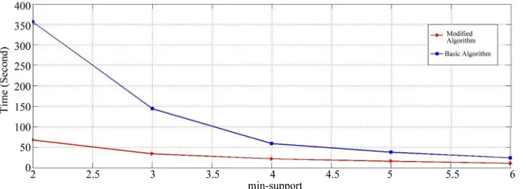
and a membership function are used for all items. The comparison is made in terms of the run time based on the number of different supports for the proposed algorithm only at levels 1 and 3 with the minimum confidence value of 0.2 with its equivalent algorithm (as introduced in [3]). The comparison has been shown in Figure 12. As the results show, the proposed algorithm will reduce the run time and mining of rules from the user’s desirable levels. In addition, the results obtained show that the rules developed by the proposed algorithm are more close to reality than the algorithm presented in [3], and the reason for this is the defining of different member-ship functions for individual items.

One of the important advantages of the proposed algo- rithm, is the ability to select mining of fuzzy association rules based on different levels, at the request of the user. In other words, in this algorithm, we can exactly specify that the rules are mined from which level and or which levels are mined, because in the proposed algorithm, we can define the minimum support value in different levels, so upon increasing the predefined minimum support in levels of the tree, we can, in practice, keep the rules mined from those levels to zero. Figure 9 and Figure 10

will show the number of mined rules based on the prede- fined minimum support in 100 transactions, only in levels 1 and 2 of the taxonomy, with the minimum confidence value of 0.2.

7. Discussion and Conclusions

This paper, we have employed fuzzy set concepts, multi- ple-level taxonomy, different minimum supports for each level and different membership function for each item to find fuzzy association rules in a given transaction data set.

The results reveal that: In terms of mining of associa-tion rules, the proposed method maintain higher preci-sion compared with the previous methods and the mined rules, are more close to reality, and this is because of using different membership functions for every individ-ual items.

One of the important criteria which have always been a matter of consideration is the run time of algorithm, or in other words, the time it takes the related rules are de- veloped by algorithm. If an algorithm has got a suitable precision, but its rune time is long, it will lead to the user’s dissatisfaction, so in the E-Business, speed is an important issue. The results of the run time of the pro-posed algorithm based on the minimum support defined in a number of different transactions have been shown in

Figure 11.

The proposed method has got the ability to mine asso-ciation rules at different levels based on the user’s ten-dency. As a result the mined rules can be more close to the user’s demand. As an example, the users may have tendency that the mined rules should only include the items defined at the first level, so for other levels, except the first level, they can consider a big value of the mini-mum support so that the frequent itemset is not mined from those levels and as a result no rules are derived in those levels. In addition, with this feature, the run time of the algorithm shall significantly decline.

At the end, we will present a comparison between the algorithm proposed in this paper and the algorithm pre-sented in [3]. In the algorithm prepre-sented in [3], all tax-onomy levels defined from a value, the minimum support

Figure 8. Relative number of rules under different minimum confidence.

Figure 9. Relative number of rules under different minimum support in level-1.

Figure 10. Relative number of rules under different minimum support in level-2.

Figure 12. A comparison of the modified algorithm and basic algorithm.

the elapse of time, the conditions for sale of items shall be different. As an example, based on different seasons of the year, the number of sales of a series of product may be variant. Therefore in our next work we are going to present a new method to generate such membership function dynamically to cope with the environment with changing conditions. Moreover, not only we can define the minimum support value for each individual level of the predefined taxonomy for the products but also we are able to define the minimum support for each item which makes out put rules to get closer to the user’s demanded rules.

REFERENCES

[1] R. Agrawal, T. Imielinksi and A. Swami, “Mining Asso-ciations between Sets of Items in Massive Databases,” The 1993 ACM SIGMOD Conference on Management of Data, Washington DC, 26-28 May 1993, pp. 207-216.

[2] I. Ha, Y. Cai and N. Cercone, “Data-Driven of Quantita-tive Rules in Relational Databases,” IEEE Transactions on Knowledge and Data Engineering, Vol. 5, 1993, pp. 29-40.

[3] K.-Y. Lin, B.-C. Chien and T.-P. Hong, “Mining Fuzzy Multiple-Level Association Rules from Quantitative Data,” Applied Intelligence, Vol. 18, No. 1, 2003, pp. 79-90. doi:10.1023/A:1020991105855

[4] J. Han and M. Kamber, “Data Mining: Concepts and Tech- niques,” The Morgan Kaufmann Series, 2001.

[5] R. Agrawal and R. Srikant, “Fast algorithms for mining

association rules,” 20thVery Large Data Bases Confer-ence, Hong Kong, 12-15 September 1999, pp. 487-499.

[6] R. Intan, “Mining Multidimensional Fuzzy Association Rules from a Normalized Database,” International Con-ference on Convergence and Hybrid Information Tech-nology, Daejeon, 28-30 August 2008, pp. 425-432.

doi:10.1109/ICHIT.2008.229

[7] Y. Ping Huang and L. Kao, “Using Fuzzy Support and Confidence Setting to Mine Interesting Association Rules,” IEEE Annual Meeting, Vol. 2, 2004, pp. 514-519.

[8] N. Khare, N. Adlakha and K. R. Pardasani, “An Algo-rithm for Mining Multidimensional Fuzzy Association Rules,” International Journal of Computer Science and Information Security, Vol. 5, No. 1, 2009, pp. 72-76.

[9] T. Watanabe, “A Fast Fuzzy Association Rules Mining Algorithm Utilizing Output Field Specification,” Bio-medical Soft Computing and Human Sciences, Vol. 16, No. 2, 2010, pp. 69-76.

[10] B. Liu, W. Hsu and Y. Ma, “Mining Association Rules with Multiple Minimum Supports,” Fifth ACM SIGKDD International Conference Knowledge Discovery and Data Mining, San Diego, 20 August 1999, pp. 125-134. doi:10.1145/312129.312216

[11] T. Pei Hong, T. Jung Huang and Ch. Sheng Chang, “Min-ing Multiple-level Association Rules Based on Pre-large Concepts,” InTech, 2009, pp. 438.