doi:10.1006/yjtbi.3123, available online at http://www.idealibrary.com on
Electrodiffusion Model Simulation of Rectangular Current Pulses
in a Voltage-Biased Biological Channel
Carl L. Gardner*w
z
, Joseph W. Jerom ey8
and Robert S. Eisenbergz**
wDepartment of Mathematics,Arizona State University,Tempe AZ85287-1804,U.S.A,yDepartment of Mathematics, Northwestern University, Evanston IL60208,U.S.A. and zDepartment of Molecular
Biophysics and Physiology,Rush Medical College, Chicago IL 60612,U.S.A.
(Received on 1 May2002, Accepted in revised form on26 June2002)
Numerical methods are presented for simulating stochastic-in-time current pulses for an electrodiffusion model of the biological channel, with a fixed applied voltage across the channel. The electrodiffusion model consists of the parabolic advection–diffusion equation coupled either to Gauss’ law or Poisson’s equation, depending on the choice of boundary conditions. The TRBDF2 method is employed for the advection–diffusion equation. The rectangular wave shape of previously simulated traveling wave current pulses is preserved by the full set of partial differential equations for electrodiffusion.
r2002 Elsevier Science Ltd. All rights reserved.
Introduction
Biological cells exchange chemicals and electric charge with their environments through ionic channelsFhollow cylindrical protein
molecules-Fin the cell membrane walls. Signaling in the nervous system, coordination of muscle contrac-tion including the pumping accontrac-tion of the heart, and ionic transport in every cell and organ are carried out through ionic channels.
Rectangular wave ionic current pulses have been observed experimentally in a wide variety
of channels in the membranes of many types of cells (see Hille, 1992 and references therein). The current pulses have uniform heights and are distributed stochastically in time. Using an electrodiffusion model developed in Gardner
et al. (2000), we will simulate stochastic-in-time rectangular current pulses in a finite length channel.
We will model the flow of Kþ ions (in water) through a channel of diameter 7A and length( 10A(:Kþchannels play a central role in electrical signaling in the nervous system. A typical nerve cell has hundreds of thousands of Kþ channels. Our electrodiffusion model is based on the drift-diffusion or Poisson–Nernst–Planck partial differential equations plus a model for the protein charge density in the channel. The electrodiffusion equations have traveling rectan-gular wave solutions (Gardner et al., 2000), which serve here as an inflow boundary condi-tion for rectangular wave solucondi-tions for the full partial differential equations (PDEs). We will *Corresponding author. Tel.: +1-480-965-0226; fax:
+1-480-965-0461.
E-mail addresses: [email protected] (C. L. Gardner), [email protected] (J. W. Jerome), [email protected] (R. S. Eisenberg).
z Research supported in part by the National Science Foundation under Grant DMS-9706792 and by DARPA under Grant N65236-98-1-5409.
8Research supported in part by the National Science Foundation under Grant DMS-9704458.
** Research supported in part by DARPA under Grant N65236-98-1-5409.
discuss numerical methods for the electrodiffu-sion model PDEs and present simulations of a 10A long biological channel with a fixed applied( voltage across the channel for two different sets of boundary conditions. The traveling wave rectangular current pulses are no longer solu-tions for the finite length voltage biased channel, but the rectangular wave nature of input pulses is preserved by the full PDEs.
The finite channel simulations are important because the traveling wave pulses have a length equal tov0DtP\3000 channel lengths, where v0
is the traveling wave velocity and DtP is the
average duration of a current pulse. This is consistent with experimental measurements of current pulses if the ionic velocities are on the order of the ionic permeation velocity vp; since
the channel is on for a long timeDtP compared
to an ionic transit time 10A/( vp:
The electrodiffusion model can produce not only rectangular current pulses with flat tops, but the wide variety of current behavior ob-served experimentally in channels of biological membranes. The addition of noise to the drift-diffusion equations excites current pulses with different durations and separations but equal heights, in accord with experimental measure-ments of channel currents.
The principal contribution of this paper is the extension of pulse solutions to the finite channel, where boundary conditions, corresponding to physical barriers, typically induce the breakup or modification of traveling waves. Because of this, the full parabolic problem must be simulated, which is considerably more complex than the system of ordinary differential equations which models the traveling pulses in an infinite channel. In order to illustrate this, we recall the linear model of traveling wave solutions of the classical wave equation. On the infinite physical ‘‘string’’, the solution may be written as the superposition of functions fðxþctÞ and gðxctÞ; and D’Alembert’s formula explicitly computes f
and g in terms of the initial configuration and the initial velocity of the string. If a finite string of lengthcis fastened at the ends, then the odd, 2cperiodic extension of the initial data gives the same analytical model as the infinite string, but the waves must be interpreted differently. At the endpoint barriers, the waves are reflected and
inverted. This precise correlation is only possible because of the linearity of the wave equation.
For nonlinear models, the situation is more complicated. A celebrated example is the Korte-weg–de Vries equation, which models shallow water waves. Solitons are traveling wave solu-tions for the infinite channel, but, in general, do not solve the initial-boundary problem. The authors of this paper are unaware of any correlation such as that between finite and infinite string wave motion. This makes the results of the present paper unique in the literature of nonlinear wave models, defined by parabolic differential equations, or dispersive perturbations, such as the Korteweg–de Vries equation.
Electrodiffusion Model
We model the flow of positive ions (cations) in a one-dimensional channel in an electric field
Eðx;tÞ against a background of negatively charged atoms on the channel protein. The discrete distribution of charges can be described (Eisenberg et al., 1995; Nonner et al., 1998; Nonner & Eisenberg, 1998) by continuum particle densities pðx;tÞ for the mobile cations and N for the negatively charged atoms of the protein.Nis believed to be a function of current density and electric field, but not explicitly of x
or t: The flow of cations is modeled mathema-tically by the drift-diffusion model: a partial differential equation for conservation of the cations and Gauss’ law for the electric field, plus a constitutive law specifying the current densityjðx;tÞ:
@p
@t þ
1
e
@j
@x¼0; ð1Þ
@
@xðeEÞ ¼e
2ðpNÞ þs; ð2Þ
j ¼mpEeD@p
@x; ð3Þ
where e is the proton charge, e is the dielectric coefficient (taken here to be constant), s51 is a
has been multiplied by e (i.e. E has units of eV cm1 in the cgs system). Alternatively, Poisson’s equation for the electrostatic potential energyf may be used instead of Gauss’ law:
@2
@x2ðefÞ ¼e
2ðNpÞ s; E ¼ @f
@x: ð4Þ
The choice of boundary conditions determines whether we use Gauss’ law (E is specified at inflow) or Poisson’s equation (f is specified at inflow and outflow). Well-posedness of the system of eqns (1) and (4) for the deterministic case is addressed in Jerome (1987).
The random noise term s represents small charge density fluctuations on the right-hand side of Gauss’ law. We set sequal to þs%;0, or s%;wheres%51 is a positive constant. The
non-zero values of s are randomly distributed with uniform probability in time with zero mean, i.e. with equal probability of being positive or negative. Generating noise 7s% with zero mean guarantees charge conservation. This model for noise generation mimics thermal fluctuations of charge density (where s% corresponds to the average of the absolute value of the thermal fluctuations), since it is the existence of small thermal fluctuations of charge density that is important, and not their quantitative magnitude.
We model the total charge distribution by
rðj;EÞ ¼eðpNðj;EÞÞ ¼
c
v0
ðjj%Þ E
% E1
; j%¼ev0p%; ð5Þ
wherec51 is a positive constant,p% is a reference
ion density, E% is a reference electric field, and
v0¼mE%=e: This charge model is derived near
thermal equilibrium from a Boltzmann factor in Gardneret al. (2000).
For the Kþ channel, the dielectric constant eE20; the mobility coefficient mE6 105cm2V1s1; and the diffusion coefficient DE1:5106cm2s1: Note that the Einstein relation holds:eD=m¼kT0;and that in our units e2¼1:80955106eV cm:
Experimentally, only the current IB1210 pA and the average duration of a current pulse
DtPB0:1210 ms are directly measurable. A
physically natural magnitude for p% would be a
unit charge e spread uniformly throughout the channel volume (2:61021cm3). We setp%to be
one-half this value so that the average number of ions in the channel when the channel is on is roughly 3.25. The number of ions in the channel is consistent with the energetics of packing the ions single file in the channel.
Experimentally, the external voltage V is applied over a length B10lc; where lc ¼10A(
is the channel length. We have assumed that the potential drop is very close to linear in x
outside of the channel and have therefore scaled
V-V=10 at x¼lc: We also assume that
there are equal concentrations of ions inside and outside the cell membrane, so that no current flows when V ¼0: We then set E% ¼ e V=ð10lcÞ:
These values for p% and E% yield an average pulse duration on the order of 0.1–10 or more milliseconds depending on the frequency of the noise term s; and a current of 2 pA at
V ¼10 mV. Our computed pulse durations and currents match roughly the mean of the experi-mental values, which vary depending on the Kþ channel type. The traveling wave velocity v0¼
0:6 cm s1 at V ¼10 mV, is the same order of
magnitude as the ion permeation velocity vp
through the channel. For these parameters, the constant c¼3:410551 in eqn (5).
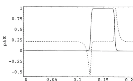
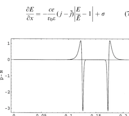
[image:3.595.310.537.544.682.2]A typical traveling wave pulse in p; which is proportional to j for the traveling wave, and the associated electric field E are shown in Fig. 1, with p0¼0:01p%; E0¼1:01E%; c% ¼E%2=p%;
and s% ¼7109E%2: The charge density for this
pulse is shown in Fig. 2. E% has been set to 104eV cm1:
The on and off times of the current pulses vary over a wide range (see Gardneret al., 2000), as is observed experimentally. By making the noise term more or less frequent, a wide variety of on and off times can be obtained.
Our model predicts physical values (v0Bvp;
DtPB0:1210 ms; etc.) which are of the
right order of magnitude for biological channels. Gating in the model is produced by a conformational change in the protein and the concomitant small charge fluctuations (cB105), rather than by a mechanical ‘‘flap’’
or ‘‘slider’’. The channel current is turned on by a small dipolar charge wave (a positive spike followed by a negative spike), while a similar reversed charge wave (a negative spike followed by a positive spike) turns off the current (see Fig. 2).
Numerical Methods for Electrodiffusion
The drift-diffusion equations (1)–(3) with our charge model (5) take the form
@p
@t þ
m
e
@
@xðEpÞ ¼D
@2p
@x2 ð6Þ
coupled to either Gauss’ law (ifE is specified at inflow)
@E
@x ¼ ce v0e
ðjj%Þ E
% E1
þs ð7Þ
or to Poisson’s equation (if f is specified at inflow and outflow)
@2f
@x2 ¼ ce v0e
ðjj%Þ E%
E1
s; E¼
@f
@x; ð8Þ
where the current density j is given in eqn (3). The noise termsis only important at the inflow boundary. Equation (6) is a parabolic PDE. Poisson’s equation (8) is elliptic, while Gauss’ law (7) is a first-order ordinary differential equation.
Variables p and E are defined at gridpoints 0;1; y; N; while f is defined at midpoints of
grid cells 1=2;1=2;3=2; y; Nþ1=2:
Given pn and En at timelevel n; a timestep consists of two parts. (i) First, we solve the transport equation (6) for pnþ1 with E¼En:
(ii) Then we solve either Gauss’ law (7) or Poisson’s equation (8) for Enþ1 using En and
pnþ1 on the right-hand side.
For the ion density p; we impose a ‘‘pulse’’ inflow boundary condition pð0;tÞ from the traveling wave solution with noise at the left boundary of the channel and a through-flow boundary condition pNþ1 ¼pN at the right
outflow boundary, where Nþ1 is a ghost point (we also setENþ1¼EN). Gating is controlled by
charge movement at the inflow boundary as in Fig. 2. We also either specify Eð0;tÞ from the traveling wave solution and use Gauss’ law, or we specify two boundary conditions, Eð0;tÞ from the traveling wave solution (which sets f1=2) and the voltage bias fNþ1=2¼fðlc;tÞ ¼ e V=10;plusthe zero of potential energyf1=2¼ fð0;tÞ ¼0 and use Poisson’s equation. The traveling wave inflow boundary condition for the parabolic PDE (6) is similar in spirit to a characteristic boundary condition for hyperbolic PDEs.
We use the TRBDF2 method for the
drift-diffusion transport equation. For Poisson’s equation we use a tridiagonal direct solve, while for Gauss’ law we integrate forward from
x¼0 to lc using TRBDF2 now as a spatial
integrator.
The TRBDF2 method consists of two partial steps. Here we describe the method for du=dt¼
fðuÞ ¼Au; where the spatial derivatives are already discretized in Au using second-order
Fig. 2. Traveling wave charge densitypNin units of
105e channel1vs. timeðxv
[image:4.595.67.290.489.691.2]accurate central differences:
@pi
@t ¼
piþ12piþpi1
Dx2
piþ1Eiþ1pi1Ei1
2Dx ;
ð9Þ
where i labels gridpoints 1;2; y; N: The
TRBDF2 method was introduced in Banket al. (1985) for nonlinear parabolic PDEs. Here the transport equation (6) is linear in p; so we just give the linear method. Further discussion of the TRBDF2 method for nonlinear diffusion can be found in Fair et al. (1991) and Johnson & Gardner (1993) (see Fig. 3).
To integrate du=dt¼Aufromt¼tntotnþ1 ¼ tnþDtn;we first apply the trapezoidal rule (TR)
to advance the solution from tn to tnþg ¼tnþ
gDtn (go1):
unþggDtn 2 Au
nþg¼unþgDtn
2 Au
n ð10Þ
and then use the second-order backward differ-entiation formula (BDF2) to advance the solu-tion fromtnþg to tnþ1:
unþ11g 2gDtnAu
nþ1
¼ 1
gð2gÞu
nþgð1gÞ2 gð2gÞu
n: ð11Þ
This composite one-step method is second-order accurate and L-stable.ww
The timestep size Dt is adjusted dynamically within a window ½Dtmin; Dtmax by monitoring
a divided-difference estimate of the local
truncation error (LTE):
LTEnþ1 ¼kDt3nuð3Þ ð12Þ
E2kDtn
1 gf
n 1
gð1gÞf
nþgþ 1 1gf
nþ1
;
ð13Þ
where
k¼3g
2þ4g2
12ð2gÞ : ð14Þ
The three values of f employed in eqn (13) have already been calculated in the most recent TRBDF2 timestep.
We use the canonical valueg¼2pffiffiffi2E0:59 which minimizes the local truncation error (Bank et al., 1985). The TRBDF2 method has the following advantages: it is a (composite) one-step method, so it is easy to start and restart; it is second-order accurate and L-stable; there are no spurious solutions from BDF2 because it is combined with TR; and Dt is adjusted dynamically by monitoring a divided-difference estimate of the LTE.
Simulation of Current Pulses in a Finite Channel
We present two sets of simulations
which depend on the choice of boundary conditions. Specifying E at inflow (Gauss’ law case) from the traveling wave solution yields numerical solutions which are very close to the traveling wave solutions. Specifying f¼0 at inflow andf¼e V=10 at outflow (the Poisson equation case) yields numerical solutions which have rectangular current pulses but greatly diminished electric fields in the channel, so the traveling wave picture is no longer applicable.
Of particular significance is the fact that in both the Gauss’ law and Poisson equation cases, the outflow ion density and the current are rectangular waves with exactly the same on and off durations as the inflow pulse. Thus the wide variety of stochastic-in-time rectangular current pulses are reproduced in the finite channel by solving the electrodiffusion model PDEs. Only
Fig. 3. TRBDF2 time levels.
wwA time integration method for du=dt¼au(Refago0) isA-stableifjjunþ1jjojjunjj:The method isL-stableif it is A-stable and limDt-Njjunþ1jj=jjunjj ¼0:TR is A-stable, but not
very special charge models like eqn (5) can preserve the shape of the input rectangular pulses in ion density.
Figures 4–13 show the inflow and outflow values of the scaled ion density p; current I;
electric field E; and charge density pN for both the Gauss’ law and Poisson equation cases with the applied voltage V ¼ 10 mV. In all figures, time is in milliseconds and ion density is measured in units of maxfpg ¼3:25 ions per channel volume. The current pulse duration for these simulations with noise every time step is about 0.5 msFhowever, by decreasing the fre-quency of the noise term, pulse durations of 10 ms or more are easily obtained (see Gardner
et al., 2000).
GAUSS’ LAWCASE
The rectangular wave shape of the ion density
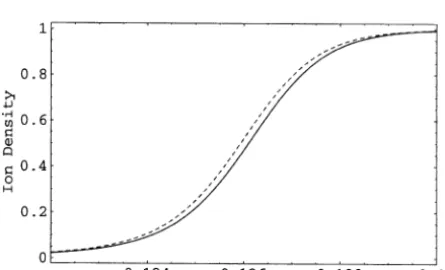
p is preserved as the ions propagate down the channel (see Fig. 4). The time delay between the inflow and outflow of the ion pulse is shown in Fig. 5 (recall that the pulse length is on the order of 3000 channel lengths). Explicitly computing the current densityj in Fig. 6 illustrates that the combination mpEeD@p=@x does produce a rectangular wave. In Figs 7 and 8, we compare the inflow electric field and charge density with the outflow values. The electric field E has preserved its traveling wave shape. However, the charge density pN is modified dramatically along the channel: at inflow it consists of two dipolar waves, while at outflow it has become a rectangular wave.
Fig. 4. Ion density at the inflow pulse boundary
condition vs. outflow for V¼ 10 mV, Gauss’ law case. The two curves are almost coincident.
Fig. 5. Closeup of ion density at the inflow pulse
boundary condition (dotted) vs. outflow forV¼ 10 mV, Gauss’ law case.
Fig. 6. Outflow current in picoamperes forV¼ 10 mV,
Gauss’ law case.
Fig. 7. Pulse boundary conditionEandEat outflow in
[image:6.595.310.536.72.214.2] [image:6.595.310.536.277.421.2] [image:6.595.65.291.328.473.2] [image:6.595.66.289.543.678.2]POISSON EQUATION CASE
The ion density p maintains its rectangular wave shape as the ions propagate down the channel (see Fig. 9). There is almost no time delay between the inflow and outflow of the ion pulse due to the Poisson equation boundary conditions. Computing the current densityj in Fig. 10 produces a rectangular wave. With V fixed at inflow and outflow, the inflow electric field is dramatically damped and re-versed in the channel (Figs 11 and 12). The charge density (Fig. 13), unlike in the Gauss’ law case, does preserve something of its original dipolar shape, even though its amplitude is greatly diminished.
Conclusion
The flat maximum value of the current in the on state vs. voltage is almost exactly linear in
Fig. 8. Pulse boundary condition pN (dotted) vs.
outflowpNin units of 105e channel1forV¼ 10 mV, Gauss’ law case.
Fig. 9. Ion density at the inflow pulse boundary
condition vs. outflow forV¼ 10 mV, Poisson’s equation case. The two curves are coincident to within a line width.
Fig. 10. Outflow current in picoamperes forV¼10 mV,
Poisson’s equation case.
Fig. 11. Eat inflow (dotted) and outflow in kVcm1for V¼ 10 mV, Poisson’s equation case.
Fig. 12. E at outflow in kVcm1 for V¼ 10 mV,
both the Gauss’ law and Poisson’s equation cases (see Fig. 14). The magnitude of the current may be understood from the fact that
j¼mpEeD@p
@xEmpmaxEEmpmax eV
10lc
ð15Þ
for the flat tops of the ion density p: (V40 implies Io0). This expression produces a linear Ohm’s law. Experimental data on channels however indicate that Ohm’s law for the biological channel is often nonlinear, e.g. sub-linearFsee Hille (1992, p. 328, Fig. 6). The sublinearity in the experimental IV curve must come from effects neglected in our model (for example, a non-uniform spatial distribution of fixed charge or a significant series resistance arising in the bath or at the interface between the bath and channel (Eisenberg, 1998).
In our finite channel model, noise in the pulse boundary condition gives the experimentally observed variation in current pulse durations and separations. A conformation change in protein and the resultant small charge fluctua-tions produce gatingFin other words, charge movement at the inflow boundary turns the channel on and off.
The present model deals with a gating model of a single prototypical channel. Much activity in current research is directed toward the descrip-tion of cell funcdescrip-tion (cf. Boyett et al., 2001). Boyettet al. (2001) attempts to identify in a cell the control mechanism for the pacemaker activity of the sinoatrial node by intracellular calcium. A mathematical model, which is really
an analog linear circuit with fitted parameters, is used to replicate the experimental evidence. Our model differs in that it accounts for thenonlinear
change of the electric field as charge flows, which is accounted for by the nonlinear Poisson equation in our model.
Future work will include computing the non-linear gating charge vs. applied voltage for the finite channel. To obtain results that match experiment, a more complicated noise model will be necessary.
REFERENCES
Bank, R. E., Cough r an, W. M., Fichtn er, W., Gro s s e,
E. H., Ro s e, D. J. & Sm ith, R. K. (1985). Transient
simulation of silicon devices and circuits. IEEE Trans. Comput. Aided Des.CAD-4,436–451.
Boy ett, M. R., Zh ang, H., Ga rn y, A & Holden, A. V.
(2001). Control of the pacemaker activity of the sinoatrial node by intracellular Ca2þ experiments and modelling. Philos. Trans.: Math. Phys. Eng Sci. (R. Soc.) 359, 1091–1110.
Eis en be rg, R. S. (1998). Ionic channels in biological
membranes: Electrostatic analysis of a natural nanotube.
Contemp. Phys.39,447–466.
Eis en be rg, R. S., Klo s ek, M. M. & Sch us s, Z. (1995).
Diffusion as a chemical reaction: stochastic trajectories between fixed concentrations. J. Chem. Phys. 102, 1767–1780.
Fa i r, R. B., Ga rdn e r, C. L., Joh ns on, M. J., Kenkel,
W. S., Ro s e, D. J., Ro s e, J. E. & Su br a h m an yan, R.
(1991). Two dimensional process simulation using ver-ified phenomenological models. IEEE Trans. Comput. Aided Des. Integrated Circuits Syst.10,643–651. Ga r dn e r, C. L., Jerom e, J. W. & Eis en be rg, R. S. (2000).
Electrodiffusion model of rectangular current pulses in ionic channels of cellular membranes.SIAM J. Appl. Math.61,792–802.
Fig. 13. Outflow pN in units of 105e/channel for V¼ 10 mV, Poisson’s equation case.
Fig. 14. Current in picoamperes vs. voltage in
Hille, B. (1992).Ionic Channels of Excitable Membranes.
Sunderland, MA: Sinauer.
Jerom e, J. (1987). Evolution systems in
semi-conductor device modeling: a cyclic uncoupled line analysis for the Gummel map. Math. Methods Appl. Sci.9,455–492.
Johnson, M. J. & Gardner, C. L. (1993). An interface
method for semiconductor process simulation. In: Cough-ran Jr., W. M., Cole, J., Lloyd, P., White, J. K. (eds.),
Semi-conductors,IMA Volumes in Mathematics and its Applica-tions, Vol. 58, pp. 33–47. New York: Springer-Verlag. Non n er, W., Ch en, D. & Eis en berg, R. S. (1998).
Anomalous mole fraction effect, electrostatics, and binding.Biophys. J.74,2327–2334.
Non n er, W. & Eis en be rg, R. S. (1998). Ion permeation