A Dual Tree Complex Discrete Cosine Harmonic
Wavelet Transform (ADCHWT) and Its
Application to Signal/Image Denoising
M. Shivamurti, S. V. Narasimhan
Digital Signal Processing and Systems Group Aerospace Electronic and Systems Division, National Aerospace Laboratories, Bangalore, India.
Email: {narasim, shivmurti}@nal.res.in
Received March 23rd, 2011; revised April 30th, 2011; accepted May 11th, 2011.
ABSTRACT
A new simple and efficient dual tree analytic wavelet transform based on Discrete Cosine Harmonic Wavelet Transform DCHWT (ADCHWT) has been proposed and is applied for signal and image denoising. The analytic DCHWT has been realized by applying DCHWT to the original signal and its Hilbert transform. The shift invariance and the envelope extraction properties of the ADCHWT have been found to be very effective in denoising speech and image signals, compared to that of DCHWT.
Keywords:Analytic Discrete Cosine Harmonic Wavelet Transform, Analytic Wavelet Transform, Dual Tree Complex Wavelet Transform, DCT, Shift Invariant Wavelet Transform, Wavelet Transform Denoising
1. Introduction
The wavelet transform (WT) provides signal compres-sion, denoising and many more desirable processing fea-tures. In spite of these advantages, the WT suffers from many major problems. The WT coefficients oscillate about the zero value around the singularities. This will reduce the magnitude of WT coefficients near singularity where their values are expected to be large, making the singularity extraction and signal modeling difficult. Fur-ther, the WT is shift variant, i.e., around singularities,
even for a small shift in input signal, there will be a large variation in the energy distribution among WT coeffi-cients at different scales resulting in different WT pat-terns which have to be considered for further processing [1]. This is due to aliasing caused by decimation at each wavelet level. Such a shift variant nature of WT not only affects detection of transients but also denoising as signal is reconstructed by decimated modified samples resulting in strong glitches [2]. Also at low signal to noise ratio like below 0dB, the conventional denoising fails. How-ever the signal compression achieved by WT is not af-fected by its shift variant property.
The WT is realized by a perfect reconstruction filter bank which involves analysis filter bank, down sampling, interpolation and synthesis filter bank. Here the aliasing
caused by the use of non-ideal filters is cancelled by the synthesis filter bank. However the reconstructed signal by such a filter bank is highly sensitive to coefficient errors and may get affected severely. Further such a WT suffers from poor directional selectivity for diagonal features. The WT filters being real, separable and their frequency response symmetric about zero in four quad-rants in the 2D frequency space, cannot distinguish be-tween two opposing diagonal directions, i.e. and
edge orientations [3,4].
o 45
o 45
The undecimated WT solves the shift variance with additional computational load. However the directional-ity problem remains unsolved as undecimated WT cannot distinguish the two opposing diagonals as it uses separa-ble filters. This blindness to such a directionality makes the processing and modeling of image features like ridges and edges difficult. For separable filters to have proper directionality, their frequency responses should be asymmetric for positive and negative frequencies and can be achieved by using complex wavelet filters [4]. How-ever the difficulty involved in the design of complex fil-ters satisfying perfect reconstruction prohibits their use in image processing.
magnitude does not oscillate and provides a smooth en-velope. Further the FT magnitude is shift invariant and also it does not suffer from aliasing and the signal recon-struction (inverse FT) does not involve any critical re-construction criterion. These benefits are due to its com-plex exponential basis instead of real basis of WT. Thus realization of complex/analytic WT has become impor-tant. This approach has been applied to image segmen-tation, classification, deconvolution, image sharpening, motion estimation, coding, water marking [4,5], texture analysis and synthesis, seismic imaging and extraction of evoked potentials in EEG [6]. The analytic WT (AWT) has the features of both WT and FT and is appropriate for time-frequency analysis like STFT [7].
The complex/analytic WT been realized using dual tree filter bank structure and Hilbert transform (HT). Many variations of this structure have been achieved with various degrees of advantages and limitations. The absence of negative frequencies for an analytic signal not only reduces aliasing but also accounts for the decima-tion by a factor of 2 at each DWT stage resulting in shift invariance. But the global nature of HT (infinite both time and frequency extent) converts the finite support wavelet function to that of an infinite support and this makes the shift invariance and alias free nature as ap-proximate. The WT realized by a two channel perfect reconstruction filter bank is computationally expensive and complicated due to explicit decimation, interpolation, associated filtering and involved delay compensation in reconstruction.
The harmonic wavelet transform (HWT) proposed by Newland [8] is simple and does not require explicit decimation, interpolation and associated filtering. The decimated components are achieved in the frequency domain by taking the inverse transform of each group of FT coefficients. The signal reconstruction is achieved by the inverse FT of properly concatenated FT coefficient groups. Here also, the WT coefficients become complex due to lack of DFT real symmetry. Further, the DFT val-ues will be generally affected by the leakage due to sig-nal truncation resulting in poor quality sigsig-nal decomposi-tion. To overcome these, the DCT based harmonic wavelet transform (DCHWT) has been proposed [9,10]. The real nature and the symmetrical signal extension of DCT respectively result in a real and more exact WT coefficients as the leakage is very much reduced [11]. The DCHWT has been used for signal/image compres-sion and spectral estimation both with computational and performance advantage. For speech and image signals, the compression provided an adaptive wavelet packet algorithm based on DCHWT has been found to be not only better than that by DCHWT but also that by
adap-tive Daubechies-2 wavelet packet. Further it has been used for efficient and accurate signal decomposition to overcome the cross-terms in Wigner-Ville time fre-quency distribution Also the DCTHWT has been extended to realize its shift invariant version. [12] which reduces the glitches when applied for denoising.
In the present work, a new dual tree analytic wavelet transform based on DCHWT (ADCHWT) has been pro-posed and is applied for signal and image denoising. The analytic DCHWT has been realized by applying DC- HWT to the original signal and its HT. The shift invari-ance property of the ADCHWT has been illustrated and its contribution in association with its envelope extrac-tion property has been found to be very effective in de-noising compared to that of DCHWT [13].
2. Dual Tree Analytic Discrete Cosine
Harmonic Wavelet Transform (ADCHWT)
In this section, the discrete cosine harmonic wavelet tran- sform and the development of the new dual tree analytic discrete cosine harmonic wavelet transform (ADCHWT) will be considered.2.1. Discrete Cosine Harmonic Wavelet Transform (DCHWT)
The filter bank realization of WT, involves down sam-pling of the components obtained by the individual ban- dpass filters. The restoration of the processed signal cor-responding to overall spectrum at the original sampling rate, involves summation of the components after their upsampling and image rejection filtering. The harmonic wavelet transform based on DFT (DFHWT) realizes the subband decomposition in the frequency domain by grouping the Fourier transform (FT) coefficients and the inverse of these groups results in decimated signals. Fur-ther after processing, the FT of the subband signals can be repositioned in their corresponding positions to re-cover the overall spectrum, with the original sampling rate. Therefore, this will not involve explicit decimation and interpolation operations. As a consequence, no band limiting and image rejection filters are necessary. Also, while reconstruction, there are no delay compensations as the subband groups are synthesized in frequency do-main by repositioning them. In view of this, the harmonic subband decomposition is very attractive due to its sim-plicity. However in the DFHWT, the grouping of the DFT coefficients with lack of conjugate symmetry makes the WT coefficients complex. For reconstruction after concatenation of the groups, the conjugate symmetry is restored to get the real signal.
trans-
formation. However, for a signal segment obtained with-out using any window function, there can be a severe leakage effect from one subband of the signal into an-other. If different subbands have to be processed differ-ently, this is not achieved as the signal energy from one to another has already leaked. The DFHWT may be tol-erable for a signal with well-separated frequency com-ponents of sufficiently high magnitude. But for closely spaced components of significantly different magnitudes, during the computation of the FT itself, the energy will leak from the higher amplitude component to the lower one (and vice versa). This results in a large bias in the spectral magnitude and may even totally eclipse smaller amplitude spectral peaks. In such a case, decomposing the signal based on DFHWT and processing the sub-bands may not be very effective. Further leakage in DFHWT will also limit its use in signal or image com-pression application. The reason for this is that it is not possible to get a good signal reconstruction by omitting the lower scales (corresponding to high frequencies) in WT as the leaked energy cannot be recovered unless all the scales are considered. Therefore to utilize the attrac-tive features of the harmonic wavelet transform, DCT is used instead of DFT, which has a comparatively reduced leakage effect. This is due to symmetrical data extension which results in a smooth transition from one DCT pe-riod to the other without any discontinuity.
The wavelet transform characterizes the correlation or similarity between the signal
,
x
W a b
x t
to beanalyzed and the wavelet function
tb a
. Such acorrelation is given by
*1 2
1
, d
x
t b
W a b x t t
a
a
(1)where is the prototype/mother wavelet. By shift-ing and scalshift-ing
t
t by the parameters and , respectively; all the basis functions
b a
t a1 2
t b
a
,
a b are obtained. Equation (1)
can be realized in the frequency domain using Parseval’s theorem as
, 1 2
*2π
j b x
a
W a b X a e d
(2a)Therefore the, the wavelet transform can be derived by windowing the spectrum X
with *
a
andinverse Fourier transforming the product.
, 1 2 1
*x
W a b a F X a (2b)
and X
are the FT of the mother waveletand the signal
t x t
. That is, for aparticular scale ‘a’ can be computed by the Equation (4b)
using
,x
W a b
X and
a by FFT algorithm.For a real symmetric signal xS
t and a real sym-metric wavelet S
t function, Equation (2a) becomes[9]
x Xs
1 2
, cos d
2π s
a
a b C a b
(3a)
(
xS ) and S
are the Fourier transform of xS
tand S
t respectively. (Generally the wavelet func-tion is a symmetrical one but to have consistency in the notation S
is used). In other words, they are the cosine transforms oft
S
x t and the mother wavelet
S t
. x
,b is the wavelet transform in cosinedomain instead of Fourier domain. Hence the corre-sponding equation for Equation (2b) is
C a
, 1 2 1
x b a C Xs a
C a s
(3b)
Therefore the cosine wavelet transform coefficient
,bx for a particular scale “a” can be computed by the Equation (3b) using
C a
s
X and s
a
by a fastcosine transform algorithm which indirectly uses FFT algorithm. s
is very simple for the Harmonic cosine wavelet transform (CHWT), and it is zero at all frequencies except constant over a small frequency band.
0 0
0 0
1, ,
, 0,
c c
s c c
otherwise
(3c)
For this the wavelet S
t is,
0sin cos π
c c
S
c
t
t t
t
Representing sin c c
t t
by sinc
ct ,
πccos 0 sin
S t t c c
t
(3d)
Hence the mother wavelet is a cosine modulated sinc function. Here the decomposition of the signal in the frequency domain is simple but suffers from the problem of poor time localization due to slow decaying of the sinc function. Though a spectral weighing other than rectan-gular improves the localization in time it results in a non-orthogonal wavelet set. The type of spectral weigh-ing will determine the wavelet as it is the cosine trans-form of the wavelet.
finite bands
π p,π q
and
π p,π q
wherecan be real numbers, not necessarily integers.
,
p q
For an orthogonal CHWT, the wavelet function is fixed and corresponds to a rectangular weighing in the frequency domain which results in such a wavelet trans-form.
The Discrete cosine transform (DCT) enables the im-plementation of the above cosine transform discussed as it forms the symmetric signalsxS
t and S
t by itself (for the given non-symmetric x t
and
t ).For a sampled signal x n
, , theDCT of points, is defined as the DFT of a point symmetrically extended signal
1
n0,1, 2 N
, ,
N 2N
y n .
, 0
2 1 , 2 1
x n n N y n
x N n N n N
1
y n is even symmetric with respect to the
1 2N
point . This leads to DCT and is given by
1
0
π 2 1
2 cos , 0 1
2
2 , 2 1
N
n x
x
k n
x n k N
C k N
C N k N k N
(4)Using the above S
N
in the CHWT, the subband decomposition is done in frequency domain unlike in time domain by a filter bank. This is achieved by group-ing the coefficients of a discrete cosine transform (DCT) of length and this is equivalent to applying a window or weighing by a constant in the frequency domain.
2N
2
The DCT coefficients can be grouped in a way similar to that of DFT coefficients and the DCT being real, there is no necessity to do the conjugate operation in placing the coefficients symmetrically [9]. The symmetrical placement is also not necessary due to the very definition of the DCT as it provides only half the number of coeffi-cients and the inverse DCT definition takes care of the symmetry. The grouped coefficients for each band have to be treated as if they are the DCT coefficients of that subband.
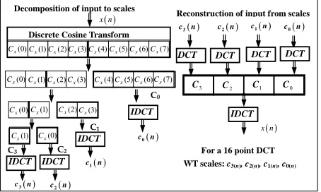
In the Figure 1 DCTHWT for a DCT size of 16 is il-lustrated and the only one side of the symmetrical coeffi-cient sequence is shown, i.e. (0 - 7). The last half part of
the coefficients correspond to scale- . The lower half of the coefficients
x x are split into two groups and the upper group correspond to scale-1, .
4 to
7x x
C C
3
3x x
C C
0 ,x
C C
0
0, . .,i e C
0C to C
2 , 1
Further the group x is split into two
groups 2 and 3 each having single coefficients
and Cx , respectively. The inverse DCT of each of the groups ; result in WT coeffi-cients of the scales , respectively. For
. .,
i e C
10, ,1 2, 3
C C C C
0,1, 2,3
C C
0
1x
C
32
Q ,
Decomposition of input to scales
) 1 ( x
C Cx(2)Cx(3) )
0 ( x
C Cx(4)Cx(5)Cx(6)Cx(7)
) 1 ( x
C Cx(0) ) 1 ( x C ) 0 ( x
C Cx(2)Cx(3)
C0
C1
C3 C2
IDCT IDCT IDCT IDCT ) 1 ( x
C Cx(2)Cx(3)Cx(4)Cx(5)Cx(6)Cx(7) )
0 ( x
C
Discrete Cosine Transform c3 n c2 n 0 c n
DCT
1
c n
DCT DCT DCT
3
C C2 C1 C0
IDCT
x n For a 16 point DCT WT scales: c3(n), c2(n), c1(n), c0(n)
Reconstruction of input from scales
3
[image:4.595.308.535.99.235.2]c n c2 n 1 c n 0 c n x n
Figure 1. DCHWT for a 1-D signal.
the scales 0 1 correspond to grouping of
coefficients as 2 3 4
, , , ,
C C C C C
Cx 8 toCx 15
,
Cx
4 to Cx
7
,
Cx 2 to Cx 3
,
Cx
1
, , respectively andthis process continues.
0
x
C
For the reconstruction, the DCTs of the subband sig-nals are concatenated to get the DCT of the fullband signal. For the first stage of inverse DCHWT illustrated in Figure 1, the DCTs of the subband signals corre-sponding to groups C3 and C4 are concatenated. The resulting group of coefficients is concatenated with the DCT of subband signal corresponding to group C2, in the next stage. Again, the resulting group of coefficients is concatenated with the DCT of subband signal corre-sponding to group C1, to form the DCT of the fullband signal.
2.2. Dual Tree Analytic Discrete Cosine
Harmonic Wavelet Transform (ADCHWT)
There are different methods of obtaining the AWT, which uses the DWT. The straight forward post filtering approach splits each filter bank output into positive and negative frequency components using a complex PRFB acting as a HT though looks simple suffers from nonzero values in the negative frequency region.
Hilbert Transform
( ) x n
ˆ( )
x n j
j j j
DC
H
W
T
DCHWT
( )
0
c n ( )
1
c n ( )
2
c n
( )
3
c n
ˆ ( )0
c n
ˆ ( )1
c n ˆ ( )2
c n
ˆ ( )3
c n
ˆ ( )j ( )
0 0
c n c n
ˆ ( )j ( )
1 1
c n c n
ˆ ( )j ( )
2 2
c n c n
ˆ ( )j ( )
3 3
[image:5.595.59.288.92.218.2]c n c n
Figure 2. Schematic of the dual tree ADCHWT for a 1D signal.
converting the input to its HT. Further, Hilbert trans-formed scales are weighted by j and are combined with
their corresponding scales by summation to get the ana-lytic harmonic discrete cosine wavelet transform (AD- CHWT). For reconstruction, the real part of the AD- CHWT is taken and the procedure is same as given in Subsection 2.1.
The HT forms an integral part of the ADCHWT and hence its quality determines the performance of AD- CHWT. The analytic signal can be realized in the fre-quency domain by making the negative frefre-quency com-ponents of the original signal to zero and scaling the positive components by a factor 2and taking its inverse FT. The imaginary part of this analytic signal gives the desired HT of the signal. However, this method suffers from leakage problem of DFT as the energy from the negative frequency components would have leaked into the positive frequency region. Therefore, it is desirable to realize HT the signal in time domain by convolving the HT impulse response with the input signal [10]. The im-pulse response h n
of the HT is given by
2 sin2
π 2
π
n
h n n
n
(5) In practice the length of the impulse response is same as data length. Hence truncating the impulse response results in Gibbs ripple effect in the frequency response of the HT. This Gibbs ripple will introduce distortion due to variation in gain in the passband of the signal. To over-come this, the HT impulse response has to be windowed by a smoothing window like Kaiser with an appropriate smoothing factor.
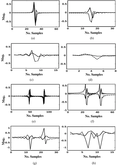
The shift invariance performance for the proposed ADCHWT is illustrated for two types of signals viz., an impulse and a rectangular pulse. The magnitude differ-ence of the WT coefficients (for different scales) be-tween original signal and its shifted version are plotted (Figure 3).
No. Samples
Ma
g
.
0 20 40 60
-0.5 0 0.5
0 10 20 30
-0.5 0 0.5
0 5 10 15
-0.5 0 0.5
0 2 4 6 8
-0.5 0 0.5
0 20 40 60
-1 -0.5 0 0.5
0 50 100
-0.5 0 0.5
0 10 20 30
-1 -0.5 0 0.5 1
0 5 10 15
-1 -0.5 0 0.5
No. Samples No. Samples No. Samples
Mag
.
(a) (b)
(c) (d)
No. Samples
Ma
g
.
No. Samples
No. Samples
Ma
g
.
No. Samples
(e) (f)
[image:5.595.307.536.96.419.2](g) (h)
Figure 3. Difference in WT indicating energy for Impulse and pulse. For impulse: (a) Scale-0, (b) Scale-1, (c) Scale-2 (d) Scale-3 For pulse: (e) Scale-0, (f) Scale-1 , (g )Scale-2, (h) Scale-3 - - - DCHWT, _____ ADCHWT.
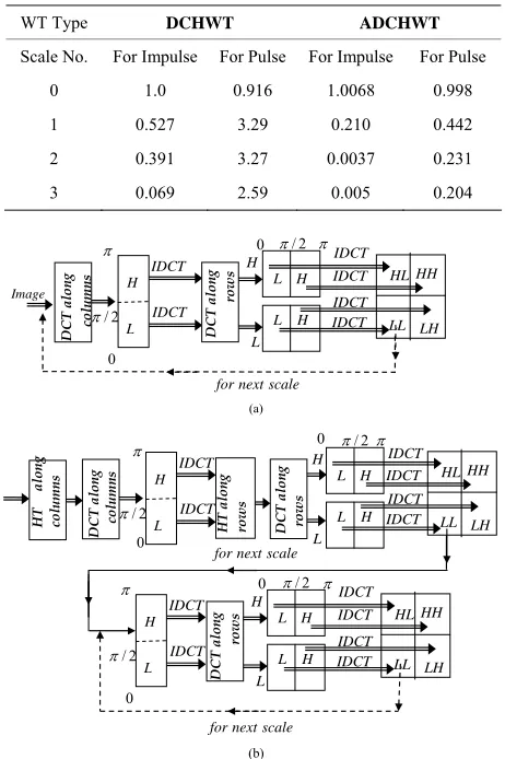
It is seen that for the higher scales the magnitude of the difference between WT coefficients for the original and shifted inputs (by 4 samples) is higher for the DCHWT than for ADCHWT both for the impulse and pulse inputs. Also the energy of this WT difference is indicated in Table 1. It is seen that with the ADCHWT, this difference energy is significantly small compared to that of DCHWT as the latter gets affected by the shift due to its shift variant nature.
2.3. Two Dimensional Dual Tree ADCHWT
For a 2D signal, the DCT coefficients for the columns are split in to two groups and their inverse DCT results in DCTHWT coefficients for the columns. The DCT along the rows for each scale are taken and grouped. The in-verse DCT of these groups will result in 2D DCTHWT (Figure 4(a)). This procedure is repeated for further scales considering the LL block as input. The procedure holds good for the real part of ADCHWT of an image.
Table 1. Error energy between the WT of original and shifted signal.
WT Type DCHWT ADCHWT
Scale No. For Impulse For Pulse For Impulse For Pulse
0 1.0 0.916 1.0068 0.998
1 0.527 3.29 0.210 0.442
2 0.391 3.27 0.0037 0.231
3 0.069 2.59 0.005 0.204
(a)
0 /2
L H L H 2 / L H 0 IDCT LL LH HL HH H L IDCT IDCT IDCT IDCT IDCT scale next for Image DCT a lon g colu mn s DC T alon g r ow s (b)
0 /2
L H L H 2 / L H 0 IDCT LL LH HL HH H L IDCT IDCT IDCT IDCT IDCT D C T al on g ro w s
0 /2
L H L H 2 / L H 0 IDCT LL LH HL HH H L IDCT IDCT IDCT IDCT IDCT D C T al ong co lumn s HT alon g row s HT alo ng co lu mns DC T alon g rows scale next for scale next for
Figure 4. (a) Schematic for (a) the real part and (b) the imaginary part of 2D-ADCHWT.
its HT has to be considered. For this to start with, prior to along the columns of the image are taken and for these Hilbert transformed columns, the DCTs are taken ( Fig-ure 4(b)).
Further the DCT coefficients are grouped in to two groups and for each group, inverse DCT is applied to get the WT scales corresponding to the image columns. For each scale along the rows, the HTs are taken and for Hilbert transformed rows, the DCTs are taken. Again these DCT coefficients are grouped in to two groups and for each group inverse DCT is applied to get ADCHWT with scales HL, HH, LL and LH. As the HT has to be applied column and row wise only once, for higher scales, that is for splitting LL further, HT should not be applied and this is indicated in the Figure 3(b) which shows the absence column and row wise application of HT beyond LL scale. That is further LL scale decomposition is simi-lar to that of the real part decomposition.
3. Signal and Image Denoising Using
ADCHWT
Wavelet domain plays an important role in noise sup-pression. This is because, unlike removal of frequency components in FT based methods, here no (higher) fre-quency component is removed which results in smooth-ing of fast changes or edges. But in wavelet domain, noise suppression is done in time domain and hence no scale/frequency is removed unless it is totally not con-tributing to the signal. In wavelet denoising, in each scale, those values, which are below a certain threshold are made zero/modified and the signal is reconstructed with these modified scales. This is based on the assumption that the noise is distributed over all scales and their mag-nitudes will be small. But the problem with wavelet de-noising is shift variant nature of WT (already been ex-plained). In WT domain as the signal is reconstructed with modified decimated scale samples, there will be glitches as in between samples are removed especially at higher scales. The solution to this is to use shift invariant/ undecimated WT but this is at the expense of additional computational load. In view of this, the analytic WT, which provides shift invariance due to its reduced band-width by a factor of half, is an appropriate solution. Here in performing denoising, the threshold for each scale is found by considering the absolute values of ADCHWT coefficients. Further, the absolute values of ADCWT are compared with the estimated threshold to make a deci-sion about whether a particular WT coefficient has to be retained/modified. This decision is applied to DCHWT (real domain) and the different modified scales are used for the signal reconstruction. In decision making not only the shift invariant nature of analytic WT but also its good envelope extraction property also contributes to it. Hence in some cases, the analytic WT based denoising performs better than those of shift invariant WT.
4. Simulation Results
The performance of the ADCHWT is shown for a dis-continuous signal (SNR = 9 dB) of 2048 points, speech segment (SNR = 10 dB) and an image (SNR = 22 dB). The noise associated with these is zero mean white Gaussian noise.
For the discontinuous signal, ADCHWT with 11 scales is considered and the denoising is done for lower 5 scales. For this, hard thresholding is done by using the standard deviation of the first scale scaled by a factor 6 as the threshold. The hard thresholding is given by
real
,where fHT
x is the modified DCHWT for denoising, is the threshold and x is the analytic WTcoeffi-cient value which is complex. ADCHWT showed im-proved performance as its O/P-SNR as 13.7 dB as against 13.1 dB for DCHWT and the glitches are of reduced magnitude compared to that of DCHWT (Figures 5(c) and (d)).
The speech, used is “Kaveriya Ugama Sthana Ko-dagu” sampled at 22050 Hzand quantized with 16 bits. A length of 1024 samples is used to generate frames with 50% overlap between successive frames. A 10 scale ADCHWT is considered for each frame. Further denois-ing by hard thresholddenois-ing is done for lower 5 scales usdenois-ing the standard deviation of the first scale scaled by a factor 7 as the threshold. ADCHWT extracts the signal enve-lope well (Figures 6 (a), (c) and (d), a typical signal part is shown by encircling in Figure 6(d)). This results in a
0 1000 2000
-1 -0.5 0 0.5 1
(c)
0 1000 2000 -1
-0.5 0 0.5 1
(a)
No. Samples
0 1000 2000
-1 -0.5 0 0.5 1
(b)
Ma
g
.
0 1000 2000 -1
-0.5 0 0.5 1
(d)
No. Samples
Ma
g
.
Figure 5. Denoising comparison for discontinuous signal (a) Clean, (b) Noisy (10 dB), (c) by DCHWT, (d) ADCHWT.
0 5 10 15
-0.5 0 0.5
0 5 10 15
-0.5 0 0.5
0 5 10 15
-0.5 0 0.5
No. Samples ×104 No. Samples ×104
0 5 10 15
-0.5 0 0.5
(a)
Ma
g
.
(b)
(c) (d)
Mag
[image:7.595.65.284.526.696.2].
Figure 6. Denoising Comparison for speech (a) Clean, (b) Noisy (9dB), (c) DCHWT, (d) ADCHWT.
better output. SNR by 4dB compared to that of DCHWT. From hearing point of view, both sound somewhat simi-lar, however DCHWT is having some glitches.
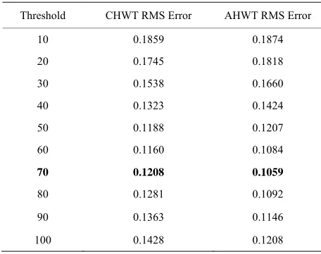
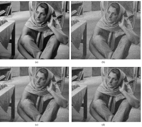
The image is decomposed into three scales with each scale consisting of four levels (LL, LH, HL and HH). So for three scales there are 12 levels. Denoising is carried out for all levels except scale-3, LL level assuming that it contains sufficiently large wavelet coefficients to repre-sent the image. For image, a threshold value of 70 which corresponds to minimum error energy between the origi-nal and reconstructed image, is found experimentally as indicated in Table 2. Further, as seen from the Table 2, the optimum threshold point for DCHWT and ADCHWT occur at 60 and 70, respectively The output SNR with threshold value 60 is 18.7128 and 19.2958 for DCHWT and ADCHWT, respectively. But the output SNR for threshold value 70 is 18.3551 and 19.50 for DCHWT and ADCHWT, respectively and for ADCHWT, the output SNR is better by 1.2 dB compared to that of DCHWT. This also evident from Figures 7(a), (c) and (d) as the overall denoising is better for ADCHWT specially in bringing out the details.
5. Conclusions
A new dual tree Analytic Cosine Harmonic Wavelet transform was proposed. The analytic DCHWT was re-alized by applying DCHWT to the original signal and its Hilbert transform.
For both impulse and pulse input signals, its shift in-variant property was found to be superior to that of DCHWT. Its application to noisy discontinuous signal, speech and image; indicated that due to its shift invariant and envelope preserving properties in deciding the modi-fication of WT has resulted in a superior denoising per-formance than those of DCHWT. The real nature and the
Table 2. Threshold selection criteria for image denoising.
Threshold CHWT RMS Error AHWT RMS Error
10 0.1859 0.1874
20 0.1745 0.1818
30 0.1538 0.1660
40 0.1323 0.1424
50 0.1188 0.1207
60 0.1160 0.1084
70 0.1208 0.1059
80 0.1281 0.1092
90 0.1363 0.1146
[image:7.595.308.536.542.722.2](a) (b)
[image:8.595.65.537.95.518.2](c) (d)
Figure 7. Comparison of DCHWT and ADCHWT for image with I/P – SNR = 22 dB. (a) Clean Image, (b) Noisy image, (c) DCHWT, (d) ADCHWT.
built in decimation and interpolation without any explicit filtering and delay compensation; makes the new algo-rithm simple and computationally efficient compared to other dual tree analytic algorithms.
REFERENCES
[1] I. W. Selesnick, R. G. Baraniuk and N. G. Kinsbury, “The Dual Tree Complex Wavelet Transform,” IEEE Signal Processing Magazine, Vol. 22, No. 6, 2005, pp. 123-151.
doi:10.1109/MSP.2005.1550194
[2] S. V. Narasimhan, A. R. Haripriya and B. K. Shreyamsha Kumar, “Improved Wigner-Ville Distribution Perform-ance Based on DCT/DF Tharmonic Wavelet Transform and Modified Magnitude Group Delay,” Signal
Process-ing, Vol. 88, No. 1, 2008, pp. 1-18.
doi:10.1016/j.sigpro.2007.06.013
[3] E. Hostalkova and A. Prochazka, “Complex Wavelet Transform in Biomedical Image Denoising,” Proceedings of 15th Annual Conference Technical Computing Prague, 14 November, 2007, pp. 1-8.
[4] N. Terzija and W. Geisselhardt, “Digital Water Image Marking Using Complex Wavelet Transform,” Interna-tional Multimedia Conference, Proceedings of the Work-shop on Multimedia and Security, Magdeburg, 20-21 September 2004, pp. 193-198.
2008, pp. 1488-1492.
[6] A. Jacquin, E. Causevic, R. John and J. Kovacevic, “Adaptive Complex Wavelet Based Filtering of EEG for Extraction of Evoked Potential Responses,” International Conference on Acoustics, Speech and Signal Processing, Philadelphia, 18-23 March 2005, pp. 393-396.
[7] X. Zhu and J. Kim, “Application of Analytic Wavelet Transform to Analysis of Highly Impulsive Noises,” Journal of Sound and Vibration, Vol. 294, No. 4-5, 2006, pp. 841-855.doi:10.1016/j.jsv.2005.12.034
[8] D. E. Newland, “Harmonic Wavelet Analysis,” Proceed-ings of Royal Society—Series A, Vol. 444, 1993, pp. 203- 225.
[9] S. V. Narasimhan, M. Harish, A. R. Haripriya and N. Basumallick, “Discrete Cosine Harmonic Wavelet Trans-form and Its Application to Signal Compression and Sub-band Spectral Estimation Using Modified Group Delay,” Signal, Image and Video Processing, Vol. 3, No. 1, 2009,
pp. 85-99.doi:10.1007/s11760-008-0062-7
[10] N. Basumallick and S. V. Narasimhan, “A Discrete Cosine Adaptive Harmonic Wavelet Packet and Its Application to Signal Compression,” Journal of Signal and Information Processing, Vol. 1, No. 1, 2010, pp. 63-76.
[11] S. V. Narasimhan and M. Harish, “A New Spectral Esti-mator Based on Discrete Cosine Transform and Modified Group Delay,” Signal Processing, Vol. 86, No. 7, 2006, pp. 1586-1596.doi:10.1016/j.sigpro.2005.09.002
[12] S. V. Narasimhan and A. Adiga, “Shift Invariant Discrete Cosine Harmonic Wavelet Transform and Its Application to Denoising,” IEEE INDICON, Bangalore, 6-8 Septem-ber 2007.