Service Networks Topological Design

doi:10.4236/ijcns.2010.311115 Published Online November 2010 (http://www.SciRP.org/journal/ijcns)

Service Networks Topological Design

Boris S. Verkhovsky

Computer Science Department, New Jersey Institute of Technology, Newark, USA E-mail: [email protected]

Received June 18, 2010; revised August 12, 2010; accepted September 23, 2010

Abstract

Topological design of service networks is studied in the paper. A quantitative model and algorithm minimiz-ing cost of processminimiz-ing and delivery are described. An algorithm solvminimiz-ing combinatorial problem of optimal design based on binary partitioning, a parametric search and dynamic programming optimization of a binary tree are described and demonstrated in numeric examples.

Keywords:Delivery/Processing Cost, Binary Partitioning, Dynamic Programming, First Responders, Average Complexity, Service Provider, Water Desalination

1. Introduction and Problem Definition

Modern satellite communication networks with their terrestrial users interconnected via terrestrial links with earth stations are an example of a service providing net-work (SPN).

Modern telecommunications is a highly competitive business. To reduce service fees and to make it eco-nomically attractive to potential customers, a communi-cation company must decide how many earth stations of each type it needs, where to allocate them, and how the customers must be interconnected with the earth stations. A correct decision can save hundreds of millions of dol-lars annually and hence can attract more users.

In more general terms we consider a set of users that require a service [1]. The type of service can be either water desalination and/or purification and delivery to customers. Or it can be a regional gas supply. Or emer-gency services (ERs, fire departments, or police station or a set of first responders). Or a set of special postal service providers (mail deliverers, UPS offices, etc.).

From a computational point of view, the problem is NP-complete, i.e., it requires brute-force algorithms or heuristics with exponential time-complexity. These ap-proaches must find an optimal way of clustering all users, [2-5]. This paper describes a set of algorithms that solve the problem of clustering-and-location of all service pro-viders with a polynomial time complexity. Preliminary results are provided in [6]. For more insights on prob-lems and algorithms related with network design see [7-12].

2. Problem Statement

1) Let us consider locations of n users with coordinates Pi = (ai, bi), i = 1, , n. Each user is characterized by a

“volume” of required service wi(“weight” of i-th user);



2) Let C_k 



u v_k, _k



be a location of k-th service cen-ter (server, for short), k = 1, 2, , m;

3) Let Sk be a set of all users connected with the k-th

server Ck;

4) Let f (wi, Pi, Ck) be a cost function of the link

con-necting the i-th user Pi and k-th server Ck;

here for all i = 1, 2, , nPi are the inputs and for all k =

1, 2, , mCk are decision variables.

 

Then a minimal total cost of all links and all servers equals





1, , 1, , 1

min min , ( )

m m k k

m

S S CC 

 

k i S f_i P Ci k qk



i S wi ,

(1) where (

k

k i S

q



_ wi) is the cost of k-th server as a non- linear function of all service flows. Thus the problem (1) requires a comprehensive analysis in order to find opti-mal clusters (subsets) S1, , Sm.

Models and methods of clustering in general has been studied and described in [5]. Surveys on models and al-gorithms related to clustering are provided in [5,9].

3. Special Cases

B. VERKHOVSKY ₈₅₁



j



k

Indeed, in











1

: : , , : min , ,

k i i k j m i i

S  i f w P C  _{ } f w P C (2)

i.e., every user is connected with the closest or least ex-pensive delivery link.

Case 2: If for k = 1, , mSk are known, then the

op-timal allocation of every server can be determined inde-pendently:





min _k , ,

k

C



i S f w P Ci i (3)

for k = 1, , m.

Case 3: If f(wi, Pi, Ck) = wi × dist(Pi, Ck), then the

problem (3) is known as aWeber problem. This problem has been investigated by many authors over the last thirty years. For references see [10,13-16].

Case4: ( ) is a linear or convex function, i.e.,

k

k i S

q



_ wi



1 2

  

1

 

2

k k

q w w q w q_k w

Then



k

 

2k

 

2k



k i S i k i S i k i S

q w q w q



    







1wi

1

which means that the more clusters the better.

The difficulties arise if the clusters Sk are not known,

the cost of every server is neither small nor flow-inde- pendent, and the number m of servers and their optimal locations (uk, vk) for all k are not known.

4. Division onto Two Clusters

It is important to stress that there is a substantial differ-ence between the two cases: m = 1 and m = 2. In the lat-ter case the problem can be solved by repetitive applica-tion of an algorithm for the Weber problem. This must be done for all possible pairs of clusters S1 and S2. There are

different ways to partite n points onto two sub-sets S1 and S2 and, for each clustering, two Weber

prob-lems must be solved. Thus, the total time complexity of this brute-force approach {even for m = 2} is O(2n), [3].

1

2n 

5. Binary Parametric Partitioning

In this section we provide a procedure that divides a network N1 with one server S1 onto two sub-networks N2

and N3 with two servers.

Step A1: {find optimal location of “center of gravity”

0 for all n users, [1]}; consider m = 1 and solve the

problem C





1

minC



ni f w P Ci, ,i . (4)

Step A2: consider a straight line L and rotate it around the center of gravity C0; {for every angle x of rotation the

line L divides all points onto two clusters S1(x) and

S2(x)};

i

P

Step A3: for every point (user) consider polar coordi-nates (i, di) using C0 as the origin of the coordinate

sys-tem; {here i is an angular coordinate of Pi};

Step A4: fori = 1 tondo : mod

i i

x   ; (5) sort all xi in ascending order;

Step A5: ifxi = i thenchi = 1

elsechi = 0;

Step A6: if (xixandchi = 1) or (xi > xand = 0)

then

i

ch

 

1

i

PS x elsePiS2

 

x ; iS

Step A7: fork = 1,2 and k

 

x compute

 





: min



, ,

k k

k k C i S i i k



g S x 



_ f w P C ; (6)

Step A8: {compute the cost of two servers and all links}:

 



 

 



1





 



2

1 2

1 1 2 2

: _{i i}

i S i S

h x q w q w

g S x g S x



 

 









(7)

Remark 1: The line L divides all n points onto two clus-ters, S1(x) and S2(x), by at most n different ways as the

angle x changes from 0 to ;

Step A9: Rotate the separating line L and find an angle that minimizes the function

  

(7) :

  

: min0 x

 

h x see h r  _{ }h x (8) Robustness of partitioning: In Step A9, the angle of rotation x of line L is the parameter. Several thousands computer experiments demonstrate that L divides all points/users onto two subsets S1 and S2 in such a way that

for k = 1, 2 the following property almost always holds: if iS r_k( ),

then f w P C( i, , )i k  f w P C( i, , i 3k) (9) However, if n is large, then with small probabilities there are one or two points (called “fugitives”), for which (9) does not hold;

Step A10: iffor iS1(r)

f(wi, Pi, C1) > f(wi, Pi, C2),

then reassign iS2(r);

iffor iS2(r)

f(wi, Pi, C2) > f(wi, Pi, C1),

then reassign iS1(r);

Remark 3: iS1(r), then

1 2

Prob [ (f w P C_i, , )_i  f w P C( _i, , )]_i , where

0, if n 400 and 1 / 200 if n 500

     

Therefore the separating like with very high probabil-ity cluster the points onto two sets, for which (9) holds.

of C1 and C2 for new values of S1(r) and S2(r); {we

de-fine S1(r) and S2(r) as the optimal binary partitioning}.

Remark 4: The computer experiments for 25 n 600 indicate remarkable robustness of the Binary Partitioning Algorithm (BPA): the Step 10 and Step 11 do not create instability of the BPA, [6].

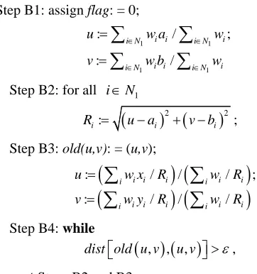
6. Search for “Center of Gravity”

Step B1: assign flag: = 0;

1 1

1 1

: /

: /

i i i

i N i N

i i i

i N i N

u w a

v w b

 

 

 









; w

w



Step B2: for all iN1



 

2 2

:

i i

R  ua  v bi





; ; Step B3: old(u,v): = (u,v);



 



 

: / / /

: / / /

i i i i i

i i

i i i i i

i i

u w x R w R

v w y R w R

 









Step B4: while

   

, , , dist old u v_ u v _,

repeat Steps B2 and B3;

Step B5 {search of a stationary point SP;  is a specified accuracy of location of the center of gravity}: Assign SP: = (u,v);

Step B6: if for all jN1{dist SP P



, j



 andflag

= 0}, thenSP is the “center of gravity”;

if for all jN1 {dist SP P



, j



 and flag 1},

thenN1:N1



pnt



; flag: = 0; goto Step B2; Step B7: if dist SP P



, _j





 

pnt

then ; pnt: =

k; .

1 flag 

1: 1

N N 

7. Minimax Search for Minimum of h(x)

Let h be a function computable on a set S of N discrete points x1,,xN

, ,

. It is obvious that N evaluations of h at points x1 xN are enough to solve any problem by

total enumeration. However, since h is a periodic func-tion with known period P, i.e., holds for every integer k, and for every i = 1, , N, an opti-mal algorithm with time complexity of order



i

 

i

h x kP h x 





logN



 .is developed and published in [16,17].

8. Binary Partitioning & Associated Binary

Tree

Let H_k: t_k s_k where Hk is a combined cost of the

network Nk. Let’s consider an algorithm that divides the

network N1 into two sub-networks N2 and N3 with

corre-sponding service delivery costs t2 and t3 and

correspond-ing costs of servers s2 and s3. We assume that the

algo-rithm divides N1 into two subnets in such a way that t2 +

t3 + s2 + s3 is minimal.

For further consideration we represent the binary par-titioning as a binary tree where the root of the tree repre-sents a cluster (set of all users) S1 and associated with it

the network N1. In general, a k-th node of the binary tree

represents a cluster Sk and associated with it a network Nk.

Two children of the k-th node represent two sub-net- works N2k and N2k + 1 of the network Nk (as result of the

binary partitioning).

From the above definitions and from the essence of the problem it is clear that for all k the following inequalities hold

2 , 2 1and 2 2

k k k k k k k 1

s s s s _ t t t _ . (10) The latter inequality holds because each sub-network N2k and N2k + 1 has a smaller number of users than Nk.

9. Non-Monotone Nature of Total Cost

If Hk > H2k + H2k + 1, then it is obvious that a partitioning

into two clusters (sub-networks) is cost-wise beneficial. However, Hk < H2k + H2k + 1 does not imply that any

further partitioning is not cost-wise beneficial. To illus-trate that let’s consider a network Nk and its six

subnet-works N2k, N2k + 1, N4k, N4k + 1, N4k + 2, N4k + 3.

Remark 6: To demonstrate various cases we consider two scenarios of inputs in the following table.

Case H1= 91 (see Table 1): since H1 > H2 + H3, then

the binary partitioning of N1 into two sub-networks is

gainful;

Case H1 = 86 (see Table 2) illustrates that a local analysis of the total costs does not provide a correct in-sight.

Table 1. t1 = 67 and for t5 = 11.

Sub-networks Ni N1 N2 N3 N4 N5 N6 N7

Delivery-link cost ti 67 25 29 12 11 10 7

Server cost sk 24 19 17 10 14 12 9

[image:3.595.60.241.186.379.2]

Total cost Hk 91 44 46 22 25 22 16

Table 2. t1 = 62 and for t5 = 7.

Sub-networks Ni N1 N2 N3 N4 N5 N6 N7

Delivery-link cost ti 62 25 29 12 7 10 7

Server cost sk 24 19 17 10 14 12 9

B. VERKHOVSKY ₈₅₃

k

In this case H1 < H2 + H3, which only implies that

there is no reason to divide the network N1 into two

sub-networks N2 and N3. However, further analysis

demonstrates that

H1 > H4 + H5 + H6 + H7 if H5 = 21;

{indeed, 86 > 22 + 21 + 22 + 16 = 81}; and H1 > H2 + H6 + H7 if H5 = 25;

{indeed, 91 > 44 + 22 + 16 = 82};

These examples illustrate that for a proper partitioning a global rather than a local analysis is required.

Definition 1:We say that a network Nkis indivisible if

there is no cost-wise advantage to divide it onto any number of sub-networks.

In addition, some sub-networks may not be further di-visible if they do not satisfy at least one of the following threshold conditions:

a) Their request for service is lower than a specified threshold;

b) The number of users in the cluster is smaller than a specified threshold.

Definition 2:We say that an optimal configuration of a service network is determined if all indivisible sub-net- works of the initial network N1 are known.

10. Dynamic Programming Algorithm

{The algorithm assigns final labels to all nodes of the associated binary tree; then determines all balanced nodes and then all prime nodes};

Bottom-up mode: a){assign to k-node a label}; : , 1, 2, ,

k k

L H k  m; (11) b) ifi-th node is a leaf then its final label

:

k

F L ; (12) c) if both children of k-th node have final labels then



2 2 1

: min ,

k k k

F  L F F_k



; (13) d) if the final labels Fk are computed for all nodes then

goto the next mode;

Top-down mode: Starting from k=1 we find a node j, for which holds

j j

F L . (14) It can be shown that it is not cost-wise advantageous to consider the descendants of this node, i.e., this node is indivisible.

Definition 3: We say that j-th node is balanced if

j j

F L holds.

Definition 4: A node that does not have a balanced ancestor is a prime node.

Proposition: The set of all prime nodes repre-sents the optimal partitioning.

opt

P

Proof: Let’s prove by reduction that (13) is always computable, i.e., when we need to compute a final label for the k-th node, the final nodes of its both children are already computed.

Indeed, consider a sub-tree T1 with five nodes {A, B, C, D, E} and sub-tree T2 with seven nodes {A, B, C, D, E, G, H}, where in both sub-trees node A is a root.

Sub-tree T1: Let B and E be the children of A; and C and D be the children of B. In addition, let the nodes C, D and E be leaves.

Then by definition (12),

: ; : and :

C C D D E E

F L F L F L . (15) Therefore, F_B: min( L_B, )F_CF_D

and F_A: min( L_A, )F_BF_E . (16) Thus, if T1 is a sub-tree of a larger tree, we can com-pute five final labels, i.e., we reduce the number of un-known final labels by five.

Sub-tree T2: Let B and E be the children of A; C and D be the children of B; G and H be children of E. In T2 nodes C, D, G and H are the leaves.

It is easy to see that this case can be reduced to the previous case by computing the final label of E. Indeed, by definition (12),

: and :

G G H H

F L F L (17) Therefore, F_E: min( L_E, )F_GF_H (18) Thus, after the final label of node E is known, we can consider it as a virtual leave. In other words, we reduced the sub-tree T2 to the sub-tree T1.

Hence, if T2 is a sub-tree of a larger tree, we can compute the all final labels of its nodes, i.e., we reduce the number of unknown final labels by seven.

It is clear that in order to compute a final label for every node we need one addition and one comparison. Hence the overall complexity to compute the final labels has order O(M), where M is the number of nodes in the initial tree. In the worst case every leave has at least 2 users. Thus the total number of nodes M on the tree does not exceed n – 1, where n is the number of the users. Therefore the complexity equals O(n).

11. Optimal Algorithm for Large n

It is easy to see that the parametric partitioning requires in general case exactly n rotations of the separating line L. As a result, the time-complexity f(n) to divide n users onto two clusters is equal f(n) = an2 + O1(n) for large n.

overall worst-case complexity is of order 



n2logn



. As it shown in [18] an average complexity of the problem can be further improved. The developed ap-proach demonstrates that the average complexity of the overall binary partitioning is of order 



nlog2n



.

12. Conclusions

The ideas and algorithms described in this paper have numerous applications. In the set of algorithms provided above the Binary Partitioning algorithm (BPA) is a core sub-algorithm for solutions of many problems dealing with configuration/topological design of networks and other clustering problems. As the core sub-algorithm, the BPA has to be repeatedly executed many times; therefore it is essential to make the BPA computationally as effi-cient as possible. There are several computational blocks within the BPA:

 To determine an optimal location of the “centre of gravity”;

 To detect of a minimum of computable function using the smallest number of its probes;

 To estimate an average complexity of a di-vide-and-conquer algorithm.

We developed an appropriate quantitative analysis to handle efficiency of the BPA.

Finally, it is shown how to apply a dynamic program-ming to tackle combinatorial complexity of reconstruct-ing the best network after numerous binary partitions.

13. Acknowledgement

I express my appreciation to D. Nowak for his assistance.

14. References

[1] M. Fiddler and V. Sander, “A Parameter Based Admis-sion Control for Differentiated Services Networks,”

Computer Networks, Vol. 44, No. 4, March 2004, pp. 463-479.

[2] A. Chaves and L. Lorena, “Clustering Search Algorithm for the Capacitated Centered Clustering Problem,” Com-puters and Operations Research, Vol. 37, No. 3, March 2010, pp. 552-558.

[3] G. Diehr, “Evaluation of a Branch-and-Bound Algorithm for Clustering,” SIAM Journal on Scientific and Statisti-cal Computing, Vol. 6, No. 2, April 1985, pp. 268-284. [4] J. Heath, M. Fu and W. Jank, “New Global Optimization

Algorithms for Model-Based Clustering,” Computational Statistics and Data Analysis, Vol. 53, No. 12, October 2009, pp. 3999-4017.

[5] A. Kusiak, A. Vannelli and K. R. Kumar, “Clustering Analysis: Models and Algorithms,” Control and Cyber-netics, Vol. 15, No. 2, 1986, pp. 139-154.

[6] B. Verkhovsky, “Satellite Communication Networks: Configuration Design of Terrestrial Subnetworks”, Jour-nal of TelecommunicationsManagement, 2010.

[7] M. Gen and R. Cheng, “Evolutionary Network Design: Hybrid Genetic Algorithms Approach,” International Journal of Computational Intelligence and Applications, Vol.3, No. 4, December 2003, pp. 357- 380.

[8] H. L. Chen and R. Tim, “Network Design with Weighted Players,” Theory of Computing Systems, Vol. 45, No. 2, June 2009, pp. 302-324.

[9] D. S. Johnson, J. K. Lenstra and A. H. G. Rinooy Kan, “The Complexity of the Network Design Problem,” Net-works, Vol. 8, No. 4, 1978, pp. 279-285.

[10] P. McGregor and D. Shen, “Network Design: An Algo-rithm for the Access Facility Location Problem,” IEEE Transactions on Communications, Vol. COM-25, No. 1, January 1977, pp. 61-73.

[11] J. Smith, F. Cruz and T. V. Woensel, “Topological Net-work Design of General, Finite, Multi-Server Queuing Networks,” European Journal of Operational Research, Vol. 201, No. 2, March 2010, pp. 427-441.

[12] B. Verkhovsky, “Constrained Shortest Path Algorithm for Network Design,” International Journal of General Sys-tems, Vol. 23, No. 2, 1996, pp. 183-195.

[13] M. Bischoff and K. Dächert, “Allocation Search Methods for a Generalized Class of Location–Allocation Prob-lems,” European Journal of Operational Research, Vol. 192, No. 3, February 2009, pp. 793-807.

[14] R. Bellman, “An Application of Dynamic Programming to Location–Allocation Problems,” SIAM Review, Vol. 7, No. 1, January 1965, pp. 126-128.

[15] J. Zhou and B. Liu, “Modeling Capacitated Loca-tion–Allocation Problem with Fuzzy Demands,” Com-puters and Industrial Engineering, Vol. 53, No. 3, Octo-ber 2007, pp. 454-468.

[16] B. Veroy (Verkhovsky), “An Optimal Algorithm for Search of Extreme of a Bimodal Function,” Journal of Complexity, Vol. 2, 1986, pp. 323-332.

[17] B. Veroy, “Optimal Search Algorithms for Extrema of a Discrete Periodic Bimodal Function," Journal of Com-plexity, Vol. 5, No. 2, June 1989, pp. 238-250.