Polynomial Based Evaluation of the Impact of Aperture Phase Taper on the Gain of Rectangular Horns

Polynomial-Based Evaluation of the Impact of

Aperture Phase Taper on the Gain of

Rectangular Horns

Konstantinos B. Baltzis

Department of Physics, Aristotle University of Thessaloniki, Thessaloniki, Greece. Email: [email protected]

Received March 28th, 2010; revised May 12th, 2010; accepted May 18th, 2010.

ABSTRACT

The aperture phase taper due to quadratic phase errors in the principal planes of a rectangular horn imposes signifi-cant constraints on the on-axis far-field gain of the horn. The precise calculation of gain reduction involves Fresnel integrals; therefore, exact results are obtained only from numerical methods. However, in horns’ analysis and design, simple closed-form expressions are often required for the description of horn-gain. This paper provides a set of simple polynomial approximations that adequately describe the gain reduction factors of pyramidal and sectoral horns. The proposed formulas are derived using least-squares polynomial regression analysis and they are valid for a broad range of quadratic phase error values. Numerical results verify the accuracy of the derived expressions. Application examples and comparisons with methods in the literature demonstrate the efficacy of the approach.

Keywords: Microwave Antennas, Rectangular Horn, Gain, Quadratic Phase Error, Linear Regression

1. Introduction

Horns are among the simplest and most widely used mi- crowave antennas. They occur in a variety of shapes and sizes and find application in areas such as wireless com- munications, electromagnetic sensing, radio frequency heating, and biomedicine. They are commonly used as feed elements for reflector and lens antennas in micro- wave systems and as high gain elements in phased arrays. Moreover, they serve as a universal standard for calibra- tion and gain measurements of other antennas [1].

Among the microwave horns, the rectangular horn is the simplest and most reliable one. This is a hollow pipe of a rectangular cross section that is flared to a larger opening in the E- or H-plane direction (sectoral horn) or in both directions (pyramidal horn). Rectan-gular horns are useful tools in science and engineering due to their simplicity in construction, ease of excita- tion, versatility, and high gain.

A classical expression for the gain of a pyramidal horn is the Schelkunoff’s horn-gain formula. This for-mula calculates the on-axis far-field gain of the horn as the product of the directivity of a uniform dominant mode rectangular waveguide without flares and the gain reduction due to the amplitude and phase taper across the horn aperture [2]. Its main assumptions are

that the horn operates at the dominant TE10 waveguide

In both horn-gain formulas [2,5], the calculation of the gain reduction factors involves Fresnel integrals and it is made numerically. However, approximate but simple closed-form expressions are often required [11, 17,18]. In this paper, we extend the analysis in [17] to include a broader range of aperture phase error values. The approximate formulas in [17] are valid for aperture phase errors up to the optimum gain condition ones. Here, we provide improved approximate polynomial expressions for the gain reduction factors of a rectang- ular horn. These formulas were obtained from the app- lication of least squares polynomial fitting over the range of aperture phase error parameters from zero to one (typical values for practical applications [19,20]). We further investigate the impact of the polynomial order on the approximation error and give representa- tive examples that show the merits of our proposal. Co- mparisons with methods in the literature and results derived from professional antenna design software [21] validate the formulation.

The rest of the paper is organized as follows: Section 2 discusses some theoretical background. Section 3 pr- esents and evaluates the proposed formulation. In Sect- ion 4, representative examples show the merits of our proposal. Finally, Section 5 concludes the paper.

[image:2.595.308.542.83.336.2] [image:2.595.305.540.511.724.2]

2. The Schelkunoff

’

s Classical and

Improved Horn-Gain Formulas

Figure 1 shows the geometry of a pyramidal horn with throat-to-aperture length P and aperture sizes A and B. The inner dimensions of the feeding rectangular wav- eguide are a and b. When A = a or B = b, we get the

[image:2.595.62.289.627.682.2]

E-or the H-plane sectoral horn, respectively. Next, in

Figure 2, we give the cross-sectional views of the horn in the two principal planes.

We assume a lossless pyramidal horn that it is well- matched to the rectangular waveguide and operates in the dominant TE10 mode. In this case, the on-axis far-field

gain of the horn is1 [2,18]

2

32

E H

AB

G L L

λ

=

π (1)

where λ is the free-space wavelength and LE and LH are

the gain reduction factors that represent the impact of the aperture phase taper due to the quadratic phase errors in the principal planes calculated [22] from:

2 2

2

1

1 0

2

exp 1 1 d

B

E

y

L jkR y

B R

  _{ } 

  

= _− _ +_{ } − _

 _   _

 

∫

(2)

A

a

P

Figure 1. Pyramidal horn geometry

E-plane view H-plane view

Figure 2. Cross-sectional views of a pyramidal horn antenna

2 2

2

2

2 0

cos exp 1 1 d

A

H

x x

L jkR x

A A R

  _{ } 

π π   _{ }

= _ _{ }− _ +  − _

 _   _

 

∫

(3)

with k= π2 λ and j= −1. Notice that (2) and (3) do not include the path long error approximation increasing the accuracy of the results. The gain reduction factors can also be written as functions of the aperture phase error parameters in the E- and H-plane that are given by

(

)

8

B B b s

λP −

= (4)

and

(

)

8

A A a t

λP −

= (5)

respectively, as [6,17]

( ) ( )

2 2

2 2

4 E

C s S s

L

s

+

= ₍₆₎

2 2

2

1 8 1 8

64 4 4

1 8 1 8

4 4

H

t t

L C C

t t t

t t

S S

t t

 

π   +   −  =  _ _− _ _

 



   +   −   +_{  }− _{  }

   

 _{ }

(7) 1_{Usually, it is assumed that the overall efficiency (i.e. the product of the}

where C

( )

⋅ and S

( )

⋅ are the cosine and sine Fresnel integrals [23], respectively.

Equation (1) can be extended by incorporating the edge effect and the impact of the fringe currents at the aper- ture edges. In this case, the gain-formula becomes [5,7]

2 2

32 1

1 1

2 E H

AB k

G L L

β λ

  

= _ + _ − _

π _{  } (8)

where β k= 1− λ

(

2a

)

2 is the TE10 mode

propaga-tion constant [24]. The improved formula is valid for both pyramidal and sectoral horns. It reduces to (1) for large apertures (β k≈1) and calculates the gain values of the E- and H-plane sectoral horns by setting LH ≈1 and LE ≈1, respectively.

3. Polynomial Description of the Gain

Reduction Factors

In [17], Aurand provided the following first- and second- order approximations for the gain reduction factors:

( ) ( )

1 1

1.032462 0.813696 1.033320 0.567302

E

H

L s

L t

= −

= − (9)

( ) ( )

2 2

2 2

1.001633 0.07082 2.97150 1.002535 0.07341 1.31704

E

H

L s s

L t t

= − −

= − − (10)

that are valid for s≤0.25 and t≤0.375. Despite their accuracy in the given range of values, these approxima- tions can not describe the gain reduction factors for phase errors far from the optimum gain condition ones (see next Section).

In this paper, we extend Aurand’s proposal and prod- uce closed-form expressions for the gain reduction fact- ors LE and LH by polynomial regression curve fitting

[25-28] of (6) and (7). The fitting curves are linear poly- nomials calculated with the least squares method [25-27]. In this method, curve-fitting involves the minimization of the sum of the squared residuals, i.e. the squared differ- ences between the exact LE (LH) value and the LE (LH)

value that is computed from the curve-fit equation for the same aperture phase error. In order to get the best fit, we use the R2 goodness-of-fit statistics metric (this is the square of the sample correlation coefficient between the data values and the calculated ones from the fitting poly- nomial). The fit improves as R2 values approach unity.

In practice, we approximate LE and LH with nth-order

polynomials, i.e. it is

( )

( )

, 0

, 0

, 1

, 1 n

n i

E E n i

i n

n i

H H n i

i

L l e s s

L l h t t

=

=

≈ = ≤

≈ = ≤

∑

∑

(11)

Let en and hn be vectors with elements the polynomial

coefficients en,i and hn,i, i = 0,1...n, respectively. In this

case, we formulate the least squares problem as:

( )

(

)

2

, ,

0

find : Minimize

N n

n E j E j

j

l L

= −

∑

e (12)

and

( )

(

)

2

, ,

0

find : Minimize

N n

n H j H j

j

l L

= −

∑

h (13)

The subscript j in (12) and (13) denotes that the spec- ific values are calculated at s or t equal to j N (the maximum value of the two aperture phase error parame- ters is one, see (11)). Each curve is evaluated at 10001 points in steps of 10-4 in the range [0,1], i.e. N = 104. Derivation of en and hn gives the nth-order polynomial

approximation of LE and LH, respectively2.

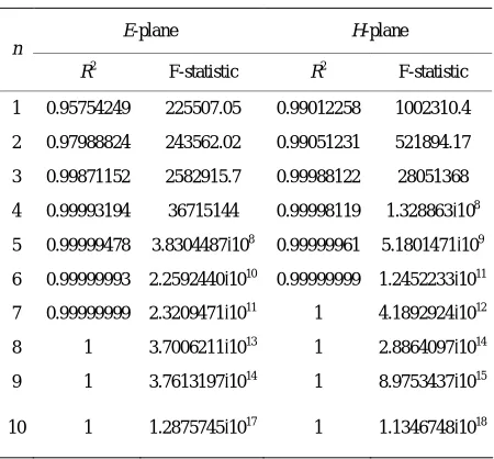
Recall that the choice of the best fit approximation uses the R2 goodness-of-fit statistics metric. Table 1 gi- ves the calculated R2 values for the best fit nth-order polynomial approximation of (6) and (7) for n = 1,2…10. The corresponding polynomial coefficients, en,i and hn,i,

are given in Tables 2 and 3. In Table 1, we also give the F-statistic values [25-27] of each approximation (F-sta- tistic value goes toward infinity as the fit becomes more ideal). Notice that LH is adequately approximated from a

polynomial with order lower than the one that is required for LE. All the results were checked and validated using

[image:3.595.307.532.512.721.2]

Matlab R2008a curve fitting routines [29].

Table 1. Goodness-of-fit values

E-plane H-plane

n

R2 F-statistic R2 F-statistic

1 0.95754249 225507.05 0.99012258 1002310.4 2 0.97988824 243562.02 0.99051231 521894.17

3 0.99871152 2582915.7 0.99988122 28051368 4 0.99993194 36715144 0.99998119 1.328863·108

5 0.99999478 3.8304487·108 _{0.99999961 5.1801471·10}9

6 0.99999993 2.2592440·1010 0.99999999 1.2452233·1011 7 0.99999999 2.3209471·1011 1 4.1892924·1012 8 1 3.7006211·1013 _{1 2.8864097·10}14

9 1 3.7613197·1014 1 8.9753437·1015 10 1 1.2875745·1017 1 1.1346748·1018

2_{A further discussion on this issue is beyond the scope of the paper; the}

[image:4.595.71.526.101.260.2]

Table 2. Polynomial coefficients en,i

i n = 1 n = 2 n = 3 n = 4 n = 5 n = 6 n = 7 n = 8 n = 9 n = 10

0 1.0336239 1.1457623 1.0240209 0.9888856 0.9976955 1.0004342 1.0000973 0.9999895 0.9999976 1.0000002 1 –1.1374395 –1.8103371 –0.3490752 0.3539478 0.0894666 –0.0256761 –0.0067831 0.0009942 0.0002653 –2.414 x10-5

2 — 0.6728975 –2.9804397 –6.1444123 –4.2926737 –3.1409013 –3.3960639 –3.5322412 –3.5161931 –3.5083720 3 — — 2.4355582 7.3574573 2.4191175 –2.1885480 –0.7707180 0.2281648 0.0783339 –0.0120796 4 — — — –2.4609496 3.0948216 11.734669 7.8352862 4.0889891 4.8195421 5.3734495

5 — — — — –2.2223085 –9.8255266 –4.2101716 3.5826714 1.5369186 –0.4574140

6 — — — — — 2.5344060 –1.5211957 –10.613170 –7.2033875 –2.7711778

7 — — — — — — 1.1587434 6.7253379 3.3850412 –2.7660781

8 — — — — — — — –1.3916486 0.3829062 5.5730509

9 — — — — — — — — –0.3943455 –2.8292557

[image:4.595.70.527.291.449.2]

10 — — — — — — — — — 0.48698211

Table 3. Polynomial coefficients hn,i

i n = 1 n = 2 n = 3 n = 4 n = 5 n = 6 n = 7 n = 8 n = 9 n = 10

0 1.0744003 1.0639483 1.0033308 0.9962335 0.9995997 1.0001198 1.0000154 0.9999976 0.9999997 1.0000000 1 –0.8163131 –0.7535950 –0.0260029 0.1160082 0.0149499 –0.0069168 –0.0010603 0.0002270 3.6932 × 10-5 –4.7892 × 10-6

2 — –0.0627181 –1.8817891 –2.5209139 –1.8133644 –1.5946318 –1.6737272 –1.6962670 –1.6920827 –1.6909553 3 — — 1.2127140 2.2069413 0.3200012 –0.5550385 –0.1155393 0.0497937 0.0107279 –0.0023056 4 — — — –0.4971136 1.6257471 3.2665367 2.0578052 1.4377260 1.6282047 1.7080531

5 — — — — –0.8491443 –2.2930680 –0.5524193 0.7374358 0.2040421 –0.0834507

6 — — — — — 0.4813079 –0.7758482 –2.2807329 –1.3916927 –0.7527678

7 — — — — — — 0.3591875 1.2805586 0.4096356 –0.4770785

8 — — — — — — — –0.2303428 0.2323408 0.9805257

9 — — — — — — — — –0.1028186 –0.4538229

10 — — — — — — — — — 0.0702009

In order to describe simple but accurately the gain redu- ction factor, we have to estimate the minimum required polynomial order. In practical terms, the goodness-of-fit statistics may not provide an efficient way to estimate the degree of error. In this case, a graphical inspection of the

0.0 0.2 0.4 0.6 0.8 1.0

0.0 0.2 0.4 0.6 0.8 1.0 1.2

G

a

in

re

du

ct

ion

fac

tor

LE

l_E(1)

l_E(2)

l_E(3)

lE (4)

s

Figure 3. E-plane gain reduction factor: Exact and appro- ximate curves

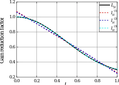
fitting curves ensures the suitability of the proposed app- roximations. Figures 3 and 4 show the exact and the (approximate) fitting curves of the gain reduction factors. Notice that the curves that describe ( )4

E

l and l_H( )3 are almost similar to the exact solution.

0.0 0.2 0.4 0.6 0.8 1.0

0.2 0.4 0.6 0.8 1.0 1.2

G

a

in

r

edu

cti

o

n

f

a

ct

or

L_H l

H (1)

l H

(2)

l_H(3)

t

[image:4.595.66.280.541.693.2] [image:4.595.319.527.543.693.2]

In order to further investigate the relation between the approximation error and the polynomial order, we used two well-known error metrics, the average absolute error and the rms error. Figure 5 shows the variation of the two metrics as a function of the polynomial order of the approximate formulas. We see that LH is adequately app-

roximated with fewer terms than LE; for example, ( ) 3 H

l

and lE( )5 yield errors less than 1%. We also notice that

the average absolute error is always slightly smaller than the rms error.

4. Application Examples

In order to show the efficacy of our approach, we give three representative examples.

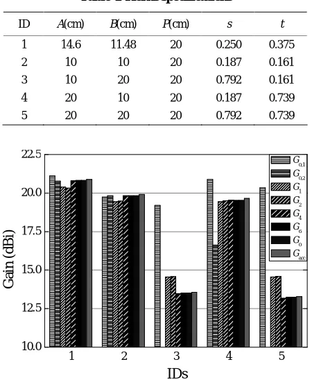
Example 1: Let us consider some typical X-band pyra- midal horns, see Table 4. Horns operate at 10 GHz and they are fed from WR-90 waveguide. Their aperture pha- se errors are calculated from (4) and (5). Figure 6 illustr- ates the gain values of the horns. With G0,1 and G0,2 we

present the values that are calculated from (1) using Aur- and’s first- and second-order approximations, respective- ely; G1, G2, G4, and G6 are the results obtained from (1)

and the proposed first-, second-, fourth-, and sixth-order approximation. G0 denotes the gain values that are calcu-

lated from (1) with adaptive quadrature integration of (2) and (3). Finally, Gacc are the exact gain values calculated

with the professional antenna design software ORAMA [21].

As it was expected, (9) and (10) are adequate only for small values of s and t (moreover, G0,2 takes complex va-

lues for great values of s; these are not shown in Figure 6). In any case, the fourth-order approximations give re- sults almost identical to the numerically calculated ones. The results are also in good consistency with the exact values calculated with ORAMA. The small gain values in cases 3 and 5 are due to the fact that the far-field gain is not maximized at the horn’s axis.

2 4 6 8 10

10-6 10-5 10-4 10-3 10-2 10-1 100 101 102

H-plane

P

er

ce

n

ta

g

e

o

f

e

rr

o

r

(%)

average asbolute error rms error

E-plane

n

[image:5.595.311.536.93.367.2]

Figure 5. Average absolute and rms error versus the order of the fitting polynomials

Table 4. Horns specifications

ID A(cm) B(cm) P(cm) s t

1 14.6 11.48 20 0.250 0.375

2 10 10 20 0.187 0.161

3 10 20 20 0.792 0.161

4 20 10 20 0.187 0.739

5 20 20 20 0.792 0.739

1 2 3 4 5

10.0 12.5 15.0 17.5 20.0 22.5

G

ai

n

(d

B

i)

iDs

G

0,1

G_0,2 G₁ G₂ G₄ G₆ G₀ G_acc

IDs

Figure 6. Calculated gain values (in dBi)

Example 2: We consider an E- and an H-plane sectoral horn that operate at 10 GHz and are fed from WR-90 wa- veguide. In the first case, B = 20 cm; in the second one, it is B = 20 cm. In both cases, the throat-to-aperture length is 20 cm.

First, we calculate the gain values from (8) with adap-tive quadrature integration of (2) and (3). The exact horns’ gains are 9.1 dB (E-plane sectoral horn) and 10.15 dB (H-plane sectoral horn). The gain values that are ob-tained from (1) and (9) are 14.83 and 11.52 dB, respec-tively; Aurand’s second-order approximation gives worst results. On the other hand, our formulation gives (the subscript denotes the order of the fitting polynomial) that

G1 = 10.19 dB, G2 = 10.22 dB, G4 = 9.03 dB and G6 =

9.09 dB (E-plane sectoral horn). In the case of the

H-plane sectoral horn, the approximation error is smaller. The calculated gains are G1 = 10.37 dB, G2 = 10.39 dB,

G4 = 10.15 dB, and G6 = 10.15 dB. Again, the fourth-

order approximations give adequate results.

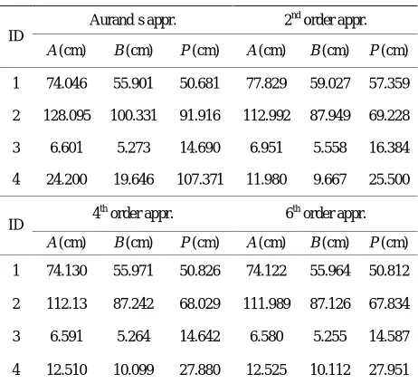
Example 3: In [11], Selvan proposed a design method for pyramidal horns of any desired gain and aperture phase error. However, the accuracy of his method is strictly related to the accuracy of the approximations of (6) and (7).

Let us consider the design examples in Table 5.

[image:5.595.67.276.542.692.2]

[image:6.595.310.536.85.259.2]

roximation) and the proposed second-, fourth-, and sixth- order approximations. Next, we used this data and calcu- lated the exact gain values with ORAMA, see Table 7. Finally, Figure 7 shows the absolute relative error bet- ween the computed and the desired gain for each case. We notice that Aurand’s approximation is adequate at small values of s and t (IDs 1 and 3). However, as the aperture phase error parameters increase (IDs 2 and 4) these approximations lead to erroneous results. In any case, the proposal in [11] is an accurate design method when a polynomial approximation with polynomial order at least equal to four is used for the description of the gain reduction factors.

Table 5. Horns design examples

ID f (GHz) Waveguide type Gdes (dBi) s t

1 1 WR-975 15.45 0.2 0.3

2 1 WR-975 15.45 0.4 0.6

3 34 WR-28 24.58 0.25 0.375

[image:6.595.55.289.269.349.2]

4 34 WR-28 24.58 0.5 0.75

Table 6. Calculated hors dimensions

Aurand’s appr. 2nd order appr. ID

A (cm) B (cm) P (cm) A (cm) B (cm) P (cm)

1 74.046 55.901 50.681 77.829 59.027 57.359

2 128.095 100.331 91.916 112.992 87.949 69.228

3 6.601 5.273 14.690 6.951 5.558 16.384

4 24.200 19.646 107.371 11.980 9.667 25.500

4th order appr. 6th order appr. ID

A (cm) B (cm) P (cm) A (cm) B (cm) P (cm) 1 74.130 55.971 50.826 74.122 55.964 50.812

2 112.13 87.242 68.029 111.989 87.126 67.834

3 6.591 5.264 14.642 6.580 5.255 14.587

4 12.510 10.099 27.880 12.525 10.112 27.951

Table 7. Desired and calculated gain values (in dBi)

ID Desired Aurand’s appr. 2

nd _order

appr.

4th _order

appr.

6th _order

appr.

1 15.45 15.62 16.09 15.63 15.63

2 15.45 16.75 15.64 15.57 15.56

3 24.58 24.67 25.12 24.66 24.64

4 24.58 30.34 24.22 24.60 24.61

1 2 3 4

0 10 20 30 40 270 280

a

b

so

lu

te

r

e

la

ti

v

e

e

rror

(

%)

iDs Aurand's appr. 2nd order appr. 4th order appr. 6th order appr.

[image:6.595.57.288.380.592.2]

IDs

Figure 7. Relative gain errors

5. Conclusions

In this paper, we presented a set of nth-order polynomial approximate expressions for the gain reduction factors of pyramidal and sectoral microwave horns. The formulas were derived with polynomial regression curve fitting techniques. Comparisons with methods in the published literature and results calculated with commercial antenna design software verified the accuracy of the proposed formulation and demonstrated the benefits of the app- roach. We also explored the relation between the polyno- mial order of the derived formulas and the approximation error. It was found that that a third-order polynomial app- roximation of the gain reduction factor in the H-plane is adequate; in order to obtain accurate results in the E-plane, a fourth-order approximation is required. This paper ex-tends previous work in the literature and applies to horns with large values of aperture phase errors. The proposed formulation is a useful tool in the analysis and design of rectangular horns, especially when simple closed-from expressions are required.

REFERENCES

[1] C. A. Balanis, “Antenna Theory: Analysis and Design,”

3rd Edition, John Wiley & Sons, Inc., Hoboken, 2005. [2] S. A. Schelkunoff, “Electromagnetic Waves,” David Van

Nostrand Company, Inc., New York, 1943.

[3] J. L. Teo and K. T. Selvan, “On the Optimum Pyramidal- Horn Design Methods,”International Journal of RF and Computer-Aided Engineering, Vol. 16, No. 6, November 2006, pp. 561-564.

[4] E. Jull, “Errors in the Predicted Gain of Pyramidal Horns,” IEEE Transactions on Antennas and Propagation, Vol. 21, No. 1, January 1973, pp. 25-31.

[image:6.595.56.288.629.719.2]

Antennas and Propagation, Vol. 47, No. 6, June 1999, pp. 1001-1004.

[6] G. Kordas, K. B. Baltzis, G. S. Miaris and J. N. Sahalos,

“Pyramidal-Horn Design under Constraints on Half-Power Beamwidth,”IEEE Transactions on Antennas and Propa- gation, Vol. 44, No. 1, February 2002, pp. 102-108. [7] K. T. Selvan, R. Sivaramakrishnan, K. R. Kini and D. R.

Poddar, “Experimental Verification of the Generalized Schelkunoff’s Horn-Gain Formulas for Sectoral Horns,” IEEE Transactions on Antennas and Propagation, Vol. 50, No. 6, June 2002, pp. 875-877.

[8] K. Guney and N. Sarikaya, “Neural Computation of Wide Aperture Dimension of Optimum Gain Pyramidal Horn,” International Journal of Infrared and Millimeter Waves, Vol. 26, No. 7, July 2005, pp. 1043-1057.

[9] A. Akdagli and K. Guney, “New Wide-Aperture-Dimen-sion Formula Obtained by Using a Particle Swarm Opti-mization for Optimum Gain Pyramidal Horns,” Micro-wave and Optical Technology Letters, Vol. 48, No. 6, June 2006, pp. 1201-1205.

[10] Y. Najjar, M. Moneer and N. Dib, “Design of Optimum Gain Pyramidal Horn with Improved Formulas Using Particle Swarm Optimization,” International Journal of RF and Computer-Aided Engineering, Vol. 17, No. 5, Sep-tember 2007, pp. 505-511.

[11] K. T. Selvan, “Accurate Design Method for Pyramidal Horns of Any Desired Gain and Aperture Phase Error,” IEEE Antennas Wireless Propagation Letters, Vol. 7, 2008, pp. 31-32.

[12] W. T. Slayton, “Design and Calibration of Microwave Antenna Gain Standards,” Report 0594740, US Naval Research Laboratory, Washington, 1954.

[13] J. W. Odendaal, “Predicting Directivity of Standard-Gain Pyramidal-Horn Antennas,”IEEE Antennas and Propa- gation Magazine, Vol. 46, No. 4, August 2004, pp. 93-98. [14] K. Harima, M. Sakasai and K. Fujii, “Determination of Gain for Pyramidal-Horn Antenna on Basis of Phase Center Location,”Proceedings of the 2008 IEEE Interna-tional Symposium on Electromagnetic Compatibility-EMC 2008, Detroit, 18-22 August 2008, pp. 1-5.

[15] G. Mayhew-Ridgers, J. W. Odendaal and J. Joubert, “Im- proved Diffraction Model and Numerical Validation for Horn Antenna Gain Calculations,” International Journal of RF and Computer-Aided Engineering, Vol. 19, No. 6, November 2009, pp. 701-711.

[16] M. Ali and S. Sanyal, “A Finite Edge GTD Analysis of the H-Plane Horn Radiation Pattern,”IEEE Transactions

on Antennas and Propagation, Vol. 58, No. 3, March 2010, pp. 969-973.

[17] J. F. Aurand, “Pyramidal Horns, Part I: Simple Expres-sions for Directivity as a Function of Aperture Phase Er-ror,”Proceedings of the 1989 IEEE Antennas Propaga-tion Society InternaPropaga-tional Symposium, San Jose, Vol. 3, 1989, pp. 1435-1438.

[18] J. F. Aurand, “Pyramidal Horns, Part II: A Novel Design Method for Horns of Any Desired Gain and Aperture Phase Error,” Proceedings of the 1989 IEEE Antennas and Propagation Society International Symposium, San Jose, Vol. 3, 26-30 June 1989, pp. 1439-1442.

[19] T. Milligan, “Scales for Rectangular Horns,”IEEE Trans- actions on Antennas and Propagation, Vol. 42, No. 5, Oc-tober 2000, pp. 79-83.

[20] T. A. Milligan, “Modern Antenna Design,” 2nd Edition, John Wiley & Sons, Inc., Hoboken, 2005.

[21] J. N. Sahalos, “Orthogonal Methods for Array Synthesis: Theory and the ORAMA Computer Tool,” John Wiley & Sons, Inc., Chichester, 2006.

[22] M. J. Maybell and P. S. Simon, “Pyramidal Horn Gain Calculation with Improved Accuracy,” IEEE Transac-tions on Antennas and Propagation, Vol. 41, No. 7, July 1993, pp. 884-889.

[23] E. W. Weisstein, “CRC Concise Encyclopedia of Mathe-matics,” 2nd Edition, Chapman & Hall/CRC, Boca Raton, 2002.

[24] D. M. Pozar, “Microwave Engineering,” 3rd Edition, John Wiley & Sons, Inc., New York, 2005.

[25] T. Hastie, R. Tibshirani and J. Friedman, “The Elements of Statistical Learning: Data Mining, Inference, and Pre- diction,” 2nd Edition, Springer, New York, 2008. [26] J. Fox, “Applied Regression Analysis and Generalized

Linear Models,” 2nd Edition, Sage Publications, Inc., Thousand Oaks, 2008.

[27] C. R. Rao, H. Toutenburg, S. Shalabh and C. Heumann,

“Linear Models and Generalizations: Least Squares and Alternatives,” 3rd Edition, Springer, Berlin, 2009. [28] F. Yang, J. Han, J. Yang and Z. Li, “Some Advances in

the Application of Weathering and Cold-Formed Steel in Transmission Tower,”Journal of Electromagnetic Analy-sis and Applications, Vol. 1, No. 1, March 2009, pp. 24-30. [29] A. Gilat and V. Subramaniam, “Numerical Methods for