Automatic Rule Induction for Unknown Word Guessing

(1)

Unknown-Word Guessing

A n d r e i M i k h e e v " University of Edinburgh

Words unknown to the lexicon present a substantial problem to NLP modules that rely on mor- phosyntactic information, such as part-of-speech taggers or syntactic parsers. In this paper we present a technique for fully automatic acquisition of rules that guess possible part-of-speech tags for unknown words using their starting and ending segments. The learning is performed from a general-purpose lexicon and word frequencies collected from a raw corpus. Three complimentary sets of word-guessing rules are statistically induced: prefix morphological rules, suffix morpho- logical rules and ending-guessing rules. Using the proposed technique, unknown-word-guessing rule sets were induced and integrated into a stochastic tagger and a rule-based tagger, which were then applied to texts with unknown words.

1. Introduction

Words unknown to the lexicon present a substantial problem to NLP modules (as, for instance, part-of-speech (pos-) taggers) that rely on information about words, such as their part of speech, number, gender, or case. Taggers assign a single POS-tag to a word-token, provided that it is known what Pos-tags this word can take on in general and the context in which this word was used. A Pos-tag stands for a unique set of morpho-syntactic features, as exemplified in Table 1, and a word can take several Pos-tags, which constitute an ambiguity class or POS-class for this word. Words with their POs-classes are usually kept in a lexicon. For every input word-token, the tagger accesses the lexicon, determines possible POS-tags this word can take on, and then chooses the most appropriate one. However, some domain-specific words or infrequently used morphological variants of general-purpose words can be missing from the lexicon and thus, their POs-classes should be guessed by the system and only then sent to the disambiguation module.

The simplest approach to POS-class guessing is either to assign all possible tags to an unknown word or to assign the most probable one, which is proper singular noun for capitalized words and common singular noun otherwise. The appealing feature of these approaches is their extreme simplicity. Not surprisingly, their performance is quite poor: if a word is assigned all possible tags, the search space for the disambiguation of a single POS-tag increases and makes it fragile; if every u n k n o w n word is classified as a noun, there will be no difficulties for disambiguation but accuracy will suffer--such a guess is not reliable enough. To assign capitalized unknown words the category proper noun seems a good heuristic, but may not always work. As argued in Church (1988), who proposes a more elaborated heuristic, Dermatas and Kokki- nakis (1995) proposed a simple probabilistic approach to unknown-word guessing:

(2)

Computational Linguistics Volume 23, Number 3

Table 1

The most frequent open-class tags from the Penn tag set.

Tag Meaning Example Tag Meaning Example

NN common noun table

NNS noun plural tables

NNP proper noun John

NNPS plural proper noun Vikings

JJ adjective green

RB adverb naturally

VB verb base form take

VBD verb past took

VBG gerund taking

VBN past participle taken VBZ verb present, 3d person takes V B P verb, present, non-3d take

the probability that an u n k n o w n word has a particular Pos-tag is estimated from the probability distribution of hapax words (words that occur only once) in the previously seen texts. 1 Whereas such a guesser is more accurate than the naive assignments and easily trainable, the tagging performance on u n k n o w n words is reported to be only about 66% correct for English. 2

More advanced word-guessing methods use word features such as leading and trailing word segments to determine possible tags for u n k n o w n words. Such methods can achieve better performance, reaching tagging accuracy of up to 85% on u n k n o w n words for English (Brill 1994; Weischedel et al. 1993). The Xerox tagger (Cutting et al. 1992) comes with a set of rules that assign an u n k n o w n word a set of possible pos-tags (i.e., POS-class) on the basis of its ending segment. We call such rules ending- guessing rules because they rely only on ending segments in their predictions. For example, an ending-guessing rule can predict that a word is a gerund or an adjective if it ends with

ing.

The ending-guessing approach was elaborated in Weischedel et al. (1993), where an u n k n o w n word was guessed by using the probability for an u n k n o w n word to be of a particular Pos-tag, given its capitalization feature and its ending. Brill (1994, 1995) describes a system of rules that uses both ending-guessing and more morphologically motivated rules. A morphological rule, unlike an ending-guessing rule, uses information about morphologically related words already known to the lexicon in its prediction. For instance, a morphologically motivated guessing rule can say that a word is an adjective if adding the suffix

ly

to it will result in a word. Clearly, ending-guessing rules have wider coverage than morphologically oriented ones, but their predictions can be less accurate.

The major topic in the development of word-Pos guessers is the strategy used for the acquisition of the guessing rules. A rule-based tagger described in Voutilainen (1995) was equipped with a set of guessing rules that had been hand-crafted using knowledge of English morphology and intuitions. A more appealing approach is automatic acquisition of such rules from available lexical resources, since it is usually less labor-intensive and less error-prone. Zhang and Kim (1990) developed a system for automated learning of morphological word formation rules. This system divides a string into three regions and infers from training examples their correspondence to un- derlying morphological features. Kupiec (1992) describes a guessing component that uses a prespecified list of suffixes (or rather endings) and then statistically learns the

1 A similar idea for estimating lexical prior probabilities for unknown words was suggested in Baayen and Sproat (1995).

(3)

predictive properties of those endings from an untagged corpus. In Brill (1994, 1995) a transformation-based learner that learns guessing rules from a pretagged training corpus is outlined: First the unknown words are labeled as common nouns and a list of generic transformations is defined. Then the learner tries to instantiate the generic transformations with word features observed in the text. A statistical-based suffix learner is presented in Schmid (1994). From a training corpus, it constructs a suffix tree where every suffix is associated with its information measure to emit a particular pos-tag. Although the learning process in these systems is fully automated and the accuracy of obtained guessing rules reaches current state-of-the-art levels, for estimation of their parameters they require significant amounts of specially prepared training data--a large training corpus (usually pretagged), training examples, and so on.

In this paper, we describe a novel, fully automatic technique for the induction of Pos-class-guessing rules for unknown words. This technique has been partially outlined in (Mikheev 1996a, 1996b) and, along with a level of accuracy for the induced rules that is higher than any previously quoted, it has an advantage in terms of quantity and simplicity of annotation of data for training. Unlike many other approaches, which implicitly or explicitly assume that the surface manifestations of morpho-syntactic features of unknown words are different from those of general language, we argue that

within the same language unknown words obey general morphological

regularities. In

our approach, we do not require large amounts of annotated text but employ fully automatic statistical learning using a pre-existing general-purpose lexicon mapped to a particular tag set and word-frequency distribution collected from a raw corpus. The proposed technique is targeted to the acquisition of both morphological and ending-guessing rules, which then can be applied cascadingly using the most accurate guessing rules first. The rule induction process is guided by a thorough guessing-rule evaluation methodology that employs precision, recall, and coverage as evaluation metrics.

In the rest of the paper we first introduce the kinds of guessing rules to be induced and then present a semi-unsupervised 3 statistical rule induction technique using data derived from the CELEX lexical database (Burnage 1990). Finally we evaluate the induced guessing rules by removing all the hapax words from the lexicon and tagging the Brown Corpus (Francis and Kucera 1982) by a stochastic tagger and a rule-based tagger.

2. Guessing-Rule Schemata

There are two kinds of word-guessing rules employed by our cascading guesser: morphological rules and nonmorphological ending-guessing rules. Morphological word- guessing rules describe how one word can be guessed given that another word is known. Unlike morphological guessing rules, nonmorphological rules do not require the base form of an unknown word to be listed in the lexicon. Such rules guess the pos-class for a word on the basis of its ending or leading segments alone. This is especially important when dealing with uninflected words and domain-specific sub- languages where many highly specialized words can be encountered. In English, as in many other languages, morphological word formation is realized by affixation: prefixation and suffixation. Thus, in general, each kind of guessing rule can be further subcategorized depending on whether it is applied to the beginning or tail of an un-

(4)

k n o w n w o r d . To m i r r o r this classification, w e will introduce a general schemata for guessing rules and a guessing rule will be seen as a particular instantiation of this schemata.

D e f i n i t i o n

A g u e s s i n g - r u l e s c h e m a t a is a structure G =x:{b.e} [-S +M ?/-class --*R-class] w h e r e

• x indicates w h e t h e r the rule is a p p l i e d to the b e g i n n i n g or e n d of a w o r d a n d has t w o possible values, b-beginning a n d e-end;

• S is the affix to be segmented; it is d e l e t e d ( - ) f r o m the b e g i n n i n g or e n d of an u n k n o w n w o r d according to the v a l u e of x;

• M is the m u t a t i v e s e g m e n t (possibly e m p t y ) , w h i c h s h o u l d be a d d e d (+) to the result string after the segmentation;

• /-class is the required Pos-class (set of one or m o r e pos-tags) of the stem; the result string after the - S a n d + M operations s h o u l d be c h e c k e d (?) in the lexicon for h a v i n g this particular Pos-class; if/-class is set to be " v o i d " no checking is required;

• R-class is the POs-class to a s s i g n (--,) to the u n k n o w n w o r d if all the a b o v e operations ( - S + M ?I) h a v e b e e n successful.

For example, the rule

e[-ied +y ?(VB VBP) --*(JJ VBD VBN)]

says that if there is an u n k n o w n w o r d w h i c h ends with ied, w e s h o u l d strip this e n d i n g from it a n d a p p e n d the string y to the r e m a i n i n g part. If w e then find this w o r d in the lexicon as (VB VBP) (base v e r b or verb of p r e s e n t tense non-3d form), w e c o n c l u d e that the u n k n o w n w o r d is of the category (JJ VBD VBN) (adjective, past verb, or participle). Thus, for instance, if the w o r d specified was u n k n o w n to the lexicon, this rule first w o u l d try to s e g m e n t the required e n d i n g ied (specified - ied = specif), then a d d to the result the m u t a t i v e s e g m e n t y (specif + y = specify), and, if the w o r d specify was f o u n d in the lexicon as (VB VBP), the u n k n o w n w o r d specified w o u l d be classified as (JJ VBD VBN).

Since the m u t a t i v e s e g m e n t can be an e m p t y string, regular m o r p h o l o g i c a l forma- tions can be c a p t u r e d as well. For instance, the rule

b[-un +"" ?(VBD VBN) --*(JJ)]

says that if s e g m e n t i n g the prefix un from an u n k n o w n w o r d results in a w o r d that is f o u n d in the lexicon as a past verb a n d participle (VBD VBN), w e c o n c l u d e that the u n k n o w n w o r d is an adjective 0J). This rule will, for instance, correctly classify the w o r d u n s c r e w e d if the w o r d screwed is listed in the lexicon as (VBD VBN).

W h e n setting the S s e g m e n t to an e m p t y string a n d the M s e g m e n t to a n o n - e m p t y string, the schemata allows for cases w h e n a s e c o n d a r y f o r m is listed in the lexicon and the base f o r m is not. For instance, the rule

e[-"" +ed ?(VBD VBN) --*(VB VBP)]

(5)

that is found in the lexicon as a past verb and participle (VBD VBN), then the u n k n o w n word is a base or non-3d present verb (VB VBP).

The general schemata can also capture ending-guessing rules if the/-class is set to be "void." This indicates that no stem lookup is required. Naturally, the mutative segment of such rules is always set to an empty string. For example, an ending- guessing rule

e[-ing +"" ?-- --*(JJ NN VBG)]

says that if a word ends with ing it can be an adjective, a noun, or a gerund. Unlike a morphological rule, this rule does not check whether the substring preceding the

i n g - e n d i n g is listed in the lexicon with a particular POs-class.

The proposed guessing-rule schemata is in fact quite similar to the set of generic transformations for unknown-word guessing developed by Brill (1995). There are, however, three major differences:

• Brill's transformations do not check whether the stem belongs to a particular POS-class while the schemata proposed here does (?/-class) and therefore imposes more rigorous constraints;

• Brill's transformations do not account for irregular morphological cases like try-tries whereas our schemata does (+M segment);

• Brill's guessing rules produce a single most likely tag for an unknown word, whereas our guesser is intended to imitate the lexicon and produce all possible tags.

Brill's system has two transformations that our schemata do not capture: when a particular character appears in a word and when a word appears in a particular context. The latter transformation is, in fact, due to the peculiarities of Brill's tagging algorithm and, in other approaches, is captured at the disambiguation phase of the tagger itself. The former feature is indirectly captured in our approach. It has been noticed (as in [Weischedel et al., 1993], for example) that capitalized and hyphenated words have a different distribution from other words. Our morphological rules account for this difference by checking the stem of the word. The ending-guessing rules, on the other hand, do not use information about stems. Thus if the ending s predicts that a word can be a plural noun or a 3d form of a verb, the information that this word was capitalized can narrow the considered set of POS-tags to plural proper noun. We therefore decided to collect ending-guessing rules separately for capitalized words, hyphenated words, and all other words. In our experiments, we restricted ourselves to the production of six different guessing-rule sets, which seemed most appropriate for English:

• Suffix ° - suffix morphological rules with no mutative endings (0). Such rules account for the regular suffixation as, for instance,

book + ed = booked;

• Suffix I - suffix morphological rules with a mutative ending in the last letter. Such rules account for many cases of the irregular suffixation as, for instance, t r y - y + ied = tried;

• Prefix - prefix morphological rules with no mutative segments (0). Such rules account for the regular prefixation as, for instance,

(6)

• Ending- - ending-guessing rules for hyphenated words;

• Ending c - ending-guessing rules for capitalized words;

• Ending* - ending-guessing rules for all other (nonhyphenated and noncapitalized) words.

3. Guessing-Rule Induction

As already mentioned, we see features that our guessing-rule schemata is intended to capture as general language regularities rather than properties of rare or corpus- specific words only. This significantly simplifies training data requirements: we can induce guessing rules from a general-purpose lexicon. 4 First, we no longer depend on the size or even existence of an annotated training corpus. Second, we do not require any annotation to be done for the training; instead, we reuse the information stated in the lexicon, which we can automatically map to a particular tag set that a tagger is trained to. We also use the actual frequencies of word usage, collected from a raw corpus. This allows for the discrimination between rules that are no longer productive (but have left their imprint on the basic lexicon) and rules that are productive in real-life texts. For guessing rules to capture general language regularities, the lexicon should be as general as possible (i.e., should list

all

possible pos-tags for a word) and large. The corresponding corpus should also be large enough to obtain reliable estimates of word-frequency distribution for at least 10,000-15,000 words.

Since a word can take on several different POS-tags, in the lexicon it can be represented as a [string/Pos-class] record, where the POs-class is a set of one or more POS-tags. For instance, the entry for the word

book,

which can be a noun (NN) or a verb (VB) would look like [book (NN VB)]. Thus the nth entry of the lexicon

(Wn)

can be represented as [W

C]n

where W is the surface lexical form and C is its pos-class. Different lexicon entries can share the same POs-class but they cannot share the same surface lexical form. In our experiments, we used a lexicon derived from CRLEX (Burnage 1990), a large multilingual database that includes extensive lexicons of English, Dutch, and German. We constructed an English lexicon of 72,136 word forms with morphological features, which we then m a p p e d into the Penn Treebank tag set (Marcus, Marcinkiewicz, and Santorini 1993). The most frequent open-class tags of this tag set are shown in Table 1. Word-frequency distribution was estimated from the Brown Corpus, which reflects multidomain language use.

As usual, we separated the test sample from the training sample. Here we followed the suggestion that the u n k n o w n words actually are quite similar to words that occur only once (hapax words) in the corpus (Dermatas and Kokkinakis 1995; Baayen and Sproat 1995). We put all the hapax words from the Brown Corpus that were found in the CnLEx-derived lexicon into the test collection (test lexicon) and all other words from the CELEx-derived lexicon into the training lexicon. In the test lexicon, we also included the hapax words not found in the CELEx-derived lexicon, assigning them the POS-tags they had in the Brown Corpus. Then we filtered out words shorter than four characters, nonwords such as numbers or alpha-numerals, which usually are handled at the tokenization phase, and all closed-class words, s which we assume will always be present in the lexicon. Thus after all these transformations we obtained a lexicon of 59,268 entries for training and the test lexicon of 17,868 entries.

4 As o p p o s e d to a corpus-specific one.

(7)

Our guessing-rule induction technique uses the training and test data prepared as described above and can be seen as a sampling for the best performing rule set from a collection of automatically produced rule sets. Here is a brief outline of its major phases:

Rule Extraction Phase (Section 3.1) - sets of word-guessing rules, (e.g., Prefix, Suffix °, Suffix 1, Ending, etc.) are extracted from the lexicon and cleaned of redundant and infrequently used rules;

Rule Scoring Phase (Section 3.2) - each rule from the extracted rule sets is ranked according to its accuracy, and rules that scored above a certain threshold are included in the working rule sets;

Rule Merging Phase (Section 3.3) - rules that have not scored high enough are merged together into more general rules, then rescored, and, depending on their score, added to the working rule sets;

Direct Evaluation Phase (Sections 3.4) - working rule sets produced with different thresholds are evaluated to obtain the best-performing ones.

3.1 Rule Extraction Phase

For the extraction of the initial sets of prefix and suffix morphological guessing rules (Prefix, Suffix °, and Suffix1), we define the operator Vn where the index n specifies the length of the mutative ending of the main word. Thus when the index n is set to 0 the result of the application of the V0 operator will be a morphological rule with no mutative segment. The V1 operator will extract the rules with the alterations in the last letter of the main word. When the ~ operator is applied to a pair of entries from the lexicon ([W

C]i

and [W C]j), first, it segments the last (or first) n characters of the shorter word

(Wj)

and stores this in the M element of the rule. Then it tries to segment an affix by subtracting the shorter word

(Wj)

without the mutative ending from the longer word

(Wi).

If the subtraction results in an non-empty string and the mutative segment is not duplicated in the affix, the system creates a morphological rule with the POs-class of the shorter word

(Cj)

as the/-class, the POS-class of the longer word (Ci) as the R-class and the segmented affix itself in the S field. For example:

[booked (JJ VBD VBN)] V0 [book (NN VB)] --+ e[-ed +"" ?(NN VB) ---+(JJ VBD VBN)] [advisable (JJ)] V1 [advise (NN VB)] ---+ e[-able +"e" ?(NN VB) ---~(JJ) ]

The V operator is applied to all possible pairs of lexical entries sequentially, and, if a rule produced by such an application has already been extracted from another pair, its frequency count (f) is incremented. Thus, prefix and suffix morphological rules together with their frequencies are produced. Next, we cut out the most infrequent rules, which might bias further learning. To do that we eliminate all the rules with frequency f less than a certain threshold 8, which usually is set quite low: 2-4. Such filtering reduces the rule sets more than tenfold.

(8)

rules from a w o r d in the lexicon ([W

C]i).

For instance, from a lexicon entry Idifferent (JJ)] the operator A will produce five ending-guessing rules:

A [different 0J)] = {

e[--t + .... ?-- ~ (J J)] e[--nt + .... ?-- --+ (JJ)] e[-ent + .... ? - ~ (J J)] e[-rent + .... ?-- --* (J3)] e[-erent + .... ? - --+ 0J)]

The G operator is applied to each entry in the lexicon, a n d if a rule it produces has already been extracted from a n o t h e r entry in the lexicon, its frequency count (f) is incremented. Then the infrequent rules w i t h f < 0 are eliminated from the ending- guessing rule set.

After applying t h e / k a n d V operations to the training lexicon, we obtained rule collections of 40,000-50,000 entries. Filtering out the rules w i t h frequency counts of 1 reduced the collections to 5,000-7,000 entries.

3.2 Rule Scoring Phase

Of course, not all acquired rules are equally good at predicting w o r d classes: some rules are more accurate in their guesses a n d some rules are more frequent in their application. For every rule acquired, we n e e d to estimate w h e t h e r it is an effective rule w o r t h retaining in the w o r k i n g rule set. To do so, we perform a statistical experiment as follows: w e take each rule from the extracted rule sets, one b y one, take each word- type from the training lexicon a n d guess its POs-class using the rule, if the rule is applicable to the word. For example, if a guessing rule strips off a particular suffix a n d a current w o r d from the lexicon does not have this suffix, we classify that w o r d a n d the rule as incompatible a n d the rule as not applicable to that word. If a rule is applicable to a word, we compare the result of the guess w i t h the information listed in the lexicon. If the guessed class is the same as the class stated in the lexicon, we count it as a hit or success, otherwise it is a failure. Then, since w e are interested in the application of the rules to word-tokens in the corpus, w e multiply the result of the guess b y the corpus frequency of the word. If w e keep the sample space for each rule separate from the others, we have a binomial experiment. The value of a guessing rule closely correlates w i t h its estimated proportion of success (/5), which is the proportion of all positive outcomes (x) of the rule application to the total n u m b e r of the trials (n), which are, in fact, the n u m b e r of all the w o r d tokens that are compatible to the rule in the corpus:

x: number of successful guesses

= n: number of the compatible to the rule word-tokens

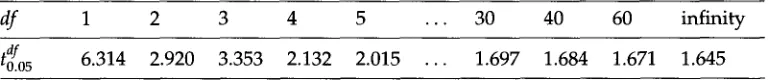
The 15 estimate is a good indicator of the rule accuracy b u t it frequently suffers from large estimation error d u e to insufficient training data. For example, if a rule was f o u n d to apply just once a n d the total n u m b e r of observations was also one, its estimate p has the maximal value (1) b u t clearly this is not a very reliable estimate. We tackle this problem b y calculating the lower confidence limit 71" L for the rule estimate,

(9)

df 1 2 3 4 5 . . . 30 40 60 infinity

[image:9.468.36.421.56.97.2]

to.a/o5 6.314 2.920 3.353 2.132 2.015 . . . 1.697 1.684 1.671 1.645

Figure 1

Values of d/ _{t(1_0.90)/2 ~ to.05}df based on sample size.

]5~ = xi+0.5 The l o w e r confidence limit 7 r L then is calculated as (Hayslett 1981):

n i + l "

7rL ₌/~* _{-- t(I_cQ/2 * Sp}.(n-l) = ~ . _ ~ ( n - 1 ) _{~(1-c~)/2 *}/ ff/~*(l~-/~*) _-

d/

w h e r e t(l_c0/2 is a coefficient of the t-distribution. It has two parameters: c~, the level of confidence a n d dr, the n u m b e r of degrees of freedom, w h i c h is one less than the sample size (dr = n - 1). e/ t(l_~)/2 can be l o o k e d u p in the tables for the t-distribution listed

df df

in e v e r y textbook on statistics. We a d o p t e d 90% confidence for w h i c h t(1_o.9o)/2=to.o5 takes values d e p e n d i n g on the sample size as in Figure 1.

Using ~-L instead of ]~ for rule scoring favors h i g h e r estimates (/3) obtained o v e r larger samples (n). Even if one rule has a high estimate v a l u e b u t that estimate was obtained over a small sample, a n o t h e r rule w i t h a l o w e r estimate value b u t obtained over a large sample m i g h t be v a l u e d h i g h e r b y ~rL. This rule-scoring function resembles the one u s e d b y T z o u k e r m a n n , Radev, a n d Gale (1995) for scoring P o s - d i s a m b i g u a t i o n rules for the French tagger. The m a i n difference b e t w e e n the two functions is that there the t value was implicitly a s s u m e d to be 1, w h i c h c o r r e s p o n d s to a confidence level of 68% on a v e r y large sample.

A n o t h e r i m p o r t a n t consideration for rating a w o r d - g u e s s i n g rule is that the longer the affix or e n d i n g (S) of this rule, the m o r e confident w e are that it is not a coincidental one, e v e n on small samples. For example, if the estimate for the w o r d - e n d i n g o was obtained over a sample of five w o r d s a n d the estimate for the w o r d - e n d i n g fulness was also obtained over a sample of five words, the latter is m o r e representative, e v e n t h o u g h the sample size is the same. Thus w e n e e d to adjust the estimation error in accordance with the length of the affix or ending. A g o o d w a y to d o this is to decrease it p r o p o r t i o n a l l y to a value that increases along with the increase of the length. A suitable solution is to use the logarithm of the affix length:

^ .(o,-,I /pt(1 - ^ *

scorei -= Pt - to.os *

V

n. Pi )/(1 +

log(ISil))

W h e n the length of S (the affix or ending) is 1, the estimation error is not c h a n g e d since l o g ( l ) is 0. For the rules with an affix or e n d i n g length of 2 the estimation error is r e d u c e d b y 1 + log(2) = 1.3, for the length 3 this will be 1 + log(3) = 1.48, etc. The longer the length, the smaller the sample that will be c o n s i d e r e d representative e n o u g h for a confident rule estimation.

(10)

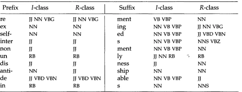
Table 2

Top scored Prefix and Suffix ° guessing rules.

Prefix /-class R-class Suffix /-class R-class

r e JJ N N VBG JJ N N VBG

e x N N N N

s e l f - N N N N

inter JJ JJ

non Jl Jl

u n RB RB

d i s JJ JJ

a n t i - N N JJ

d e jj VBD VBN JJ VBD VBN

i n RB RB

m e n t VB VBP N N

ing N N VB VBP JJ N N VBG

ed N N VB VBP JJ VBD VBN

s N N VB VBP N N S VBZ

m e n t N N VB VBP N N

ly JJ N N RB ", RB

ness JJ NN

ship N N N N

a b l e N N VB VBP JJ

s N N N N S

the threshold (0s) to 75 points, the obtained ending-guessing rule collection (Ending*) comprised 1,876 rules, the suffix rule collection without mutation (Suffix °) comprised 591 rules, the suffix rule collection with mutation (Suffix 1) comprised 912 entries and the prefix rule collection (Prefix) comprised 235 rules. Table 2 shows the highest-rated rules from the induced Prefix and Suffix ° rule sets. In general, it looks as though the induced morphological guessing rules largely consist of the standard rules of English morphology and also include a small proportion of rules that do not belong to the known morphology of English. For instance, the suffix rule e[ -et +"" ?(NN) --,(NN)] does not stand for any well-known morphological rule, but its prediction is as good as those of the standard morphological rules. The same situation can be seen with the prefix rule b[ -st +"" ?(NNS) --+(NNS)I, which is quite predictive but at the same time is not a standard English morphological rule. The ending-guessing rules, naturally, include some proper English suffixes but mostly they are simply highly predictive ending segments of words.

3.3 Rule Merging Phase

Rules which have scored lower than the threshold are merged together into more general rules. These new rules, if they score above the threshold, can also be included in the working rule sets. We merge together two rules if they scored below the threshold and have the same affix (S), mutative segment (M), and initial class (i).6 We define the rule-merging operator ®:

Ai @ Aj = At: [Si, Mi, Ii, Ri U Rj] if Si = Sj & Mi = Mj & Ii = Ij

This operator merges two rules with the same affix (S), mutative segment (M) and the initial class (I) into one rule, with the resulting class being the union of the two merged resulting classes. For example,

e[-s +"" ?(NN VB) --*(NNS)] • e[--S +"" ?(NI~ VB) ---~(NNB VBZ)I

= e[-s +"" ?(NN VB) --fiNNS VBZ)] b[--un +"" ?(VBD VBN) -*(JJ)] • b[--un +"" ?(VBD VBN) --*(VBN)]

= b[--un +"" ?(VBD VBN) --*(JJ VBN)]

[image:10.468.49.438.91.240.2]

(11)

Possible Tags JJ N N N N S RB VB VBD VBG VBN VBZ

Lexicon I n f o r m a t i o n V V V

Guesser Assigned V V V v V

Figure 2

Lexicon entry and guesser's categorization for [developed (JJ VBD VBN)].

The score of the resulting rule will be h i g h e r than the scores of the individual rules since the n u m b e r of positive observations increases a n d the n u m b e r of the trials remains the same. After a successful application of the • operator, the resulting general rule is substituted for the t w o m e r g e d ones. To p e r f o r m such rule m e r g i n g o v e r a rule set the rules that h a v e not b e e n i n c l u d e d into the w o r k i n g rule set are first sorted b y their score a n d the rules w i t h the best scores are m e r g e d first. After each successful merging, the resulting rule is rescored. This is d o n e recursively until the score of the resulting rule does not exceed the threshold, at w h i c h p o i n t it is a d d e d to the w o r k i n g rule sets. This process is applied until n o m e r g e s can be d o n e to the rules that scored poorly. In o u r e x p e r i m e n t w e noticed that the m e r g i n g a d d e d 30-40% n e w rules to the w o r k i n g rule sets, a n d therefore the final n u m b e r of rules for the i n d u c e d sets were: Prefix - 348, Suffix ° - 975, Suffix 1- 1,263 a n d Ending* - 2,196.

3.4 D i r e c t E v a l u a t i o n P h a s e

There are two i m p o r t a n t questions that arise at the rule acquisition stage: h o w to choose the scoring threshold

Os

a n d w h a t the p e r f o r m a n c e of the rule sets p r o d u c e d with different thresholds is. The task of assigning a set of POS-tags to a w o r d is actually quite similar to the task of d o c u m e n t categorization w h e r e a d o c u m e n t is assigned a set of descriptors that represent its contents. There are a n u m b e r of s t a n d a r d p a r a m e - ters (Lewis 1991) u s e d for m e a s u r i n g p e r f o r m a n c e o n this kind of task. For example, s u p p o s e that a w o r d can take on one or m o r e POS-tags f r o m the set of open-class POS-tags: qJ NN NNS RB VB VBD VBG VBN VBZ). To see h o w well the guesser performs, w e can c o m p a r e the results of the guessing with the Pos-tags k n o w n to be true for the Word (i.e., listed in the lexicon). Let us take, for instance, a lexicon e n t r y [developed (JJ VBD VBN)]. S u p p o s e that the guesser categorized it as [developed (JJ NN RB VBD VBZ)]. We can represent this situation as in Figure 2.

The p e r f o r m a n c e of the guesser can be m e a s u r e d in:

• recall - the p e r c e n t a g e of POS-tags correctly assigned b y the guesser, i.e., two (jJ VBD) out of three (JJ VBD VBN) or 66%. 100% recall w o u l d m e a n that the guesser h a d assigned all the correct pos-tags b u t not necessarily only the correct ones. So, for example, if the guesser h a d assigned all possible POS-tags to the w o r d its recall w o u l d h a v e been 100%.

• p r e c i s i o n - the p e r c e n t a g e of POS-tags the guesser assigned correctly (JJ VBD) over the total n u m b e r of POS-tags it assigned to the w o r d (Jl NN RB VBD VBZ), i.e., 2 / 5 or 40%. 100% precision w o u l d m e a n that the guesser did not assign incorrect POS-tags, a l t h o u g h not necessarily all the correct ones w e r e assigned. So, if the guesser h a d assigned only (JJ) its precision w o u l d h a v e b e e n 100%.

[image:11.468.37.419.55.105.2]

(12)

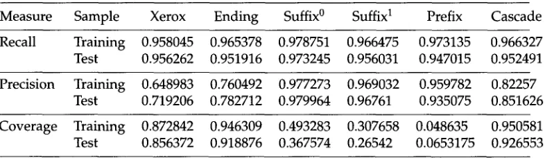
Table 3

Comparative performance of different guessing rule sets.

Measure Sample Xerox Ending Suffix ° Suffix I Prefix Cascade

Recall Training 0.958045 0.965378 0.978751 0.966475 0.973135 0.966327 Test 0 . 9 5 6 2 6 2 0.951916 0.973245 0.956031 0.947015 0.952491

Precision Training 0.648983 0.760492 0.977273 0.969032 0.959782 0.82257 Test 0 . 7 1 9 2 0 6 0.782712 0.979964 0 . 9 6 7 6 1 0 . 9 3 5 0 7 5 0.851626

Coverage Training 0.872842 0.946309 0.493283 0.307658 0.048635 0.950581 Test 0.856372 0.918876 0.367574 0.26542 0.0653175 0.926553

100 random words from the lexicon and the guesser had assigned something to 80 of them, its coverage would have been 80%.

The interpretation of these percentages is by no means straightforward, as there is no straightforward w a y of combining these different measures into a single one. For example, these measures assume that all combinations of POS-tags will be equally hard to disambiguate for the tagger, which is not necessarily the case. Obviously, the most important measure is recall since we want all possible categories for a word to be guessed. Precision seems to be slightly less important since the disambiguator should be able to handle additional noise but obviously not in large amounts. Coverage is a very important measure for a rule set, since a rule set that can guess very accurately but only for a tiny proportion of words is of questionable value. Thus, we will try to maximize recall first, then coverage, and, finally, precision. We will measure the aggregate by averaging over measures per word (micro-average), i.e., for every single word from the test collection the precision and recall of the guesses are calculated, and then we average over these values.

To find the optimal threshold (0s) for the production of a guessing rule set, we generated a number of similar rule sets using different thresholds and evaluated them against the training lexicon and the test lexicon of unseen 17,868 hapax words. Every word from the two lexicons was guessed by a rule set and the results were compared with the information the word had in the lexicon. For every application of a rule set to a word, we computed the precision and recall, and then using the total number of guessed words we computed the coverage. We noticed certain regularities in the behavior of the metrics in response to the change of the threshold: recall improves as the threshold increases while coverage drops proportionally. This is not surprising: the higher the threshold, the fewer the inaccurate rules included in the rule set, but at the same time the fewer the words that can be handled. An interesting behavior is shown by precision: first, it grows proportionally along with the increase of the threshold, but then, at high thresholds, it decreases. This means that among very confident rules with very high scores, there are many quite general ones. The best thresholds were obtained in the range of 70-80 points.

[image:12.468.50.443.93.207.2]

(13)

could handle 6% fewer unknown words. Finally, we measured the performance of the cascading application of the induced rule sets when the morphological guessing rules were applied before the ending-guessing rules (Prefix+Suffix°+Suffix 1 +Ending -c*). We detected that the cascading application of the morphological rule sets together with the ending-guessing rules increases the overall precision of the guessing by about 8%. This made the improvement over the baseline Xerox guesser 13% in precision and 7% in coverage on the test sample.

4. Unknown-Word Tagging

The direct evaluation phase gave us a basis for setting the threshold to produce the best-performing rule sets. The task of unknown-word guessing is, however, a subtask of the overall part-of-speech tagging process. Our main interest is in how the advantage of one rule set over another will affect the tagging performance. Therefore, we performed an evaluation of the impact of the word guessers on tagging accuracy. In this evaluation we used the cascading guesser with two different taggers: a c++ imple- mented bigram HMM tagger akin to one described in Kupiec (1992) and the rule-based tagger of Brill (1995). Because of the similarities in the algorithms with the LISP imple- mented Xerox tagger, we could directly use the Xerox guessing rule set with the HMM tagger. Brill's tagger came pretrained on the Brown Corpus and had a corresponding guessing component. This gave us a search-space of four basic combinations: the HMM tagger equipped with the Xerox guesser, the Brill tagger with its original guesser, the HMM tagger with our cascading (Prefix+Suffix°+Suffixl+Ending-C*) guesser and the Brill tagger with the cascading guesser. We also tried hybrid tagging using the output of the HMM tagger as the input to Brill's final state tagger, but it gave poorer results than either of the taggers and we decided not to consider this tagging option.

4.1 Setting up the Experiment

We evaluated the taggers with the guessing components on all fifteen subcorpora of the Brown Corpus, one after another. The HMM tagger was trained on the Brown Corpus in such a way that the subcorpus used for the evaluation was not seen at the training phase. All the hapax words and capitalized words with frequency less than 20 were not seen at the training of the cascading guesser. These words were not used in the training of the tagger either. This means that neither the HMM tagger nor the cascading guesser had been trained on the texts and words used for evaluation. We do not know whether the same holds for the Brill tagger and the Brill and Xerox guessers since we took them pretrained. For words that the guessing components failed to guess, we applied the standard method of classifying them as common nouns (NN) if they were not capitalized inside a sentence and proper n o u n s (NNP) otherwise. When we used the cascading guesser with the Brill tagger we interfaced them on the level of the lexicon: we guessed the unknown words before the tagging and added them to the lexicon listing the most likely tags first as required. 7 Here we want to clarify that we evaluated the overall results of the Brill tagger rather than just its unknown-word tagging component. Another point to mention is that, since we included the guessed words in the lexicon, the Brill tagger could use for the transformations all relevant Pos- tags for u n k n o w n words. This is quite different from the output of the original Brill's guesser, which provides only one Pos-tag for an unknown word.

In our tagging experiments, we measured the error rate of tagging on u n k n o w n

(14)

w o r d s using different guessers. Since, arguably, the guessing of p r o p e r n o u n s is eas- ier than is the guessing of other categories, we also m e a s u r e d the error rate for the s u b c a t e g o r y of capitalized u n k n o w n w o r d s separately. The error rate for a category of w o r d s was calculated as follows:

Error x = Wrongly_Tagged_Words_from_Set_X Total_Words_in_Set_X

Thus, for instance, the error rate of tagging the u n k n o w n w o r d s is the p r o p o r t i o n of the m i s t a g g e d u n k n o w n w o r d s to all u n k n o w n words. To see the distribution of the w o r k l o a d b e t w e e n different guessing rule sets w e also m e a s u r e d the c o v e r a g e of a guessing rule set:

CoverageR = Assigned_Wordsday_Rule_Set_R Total _Unknown _Words

We collected the error a n d c o v e r a g e m e a s u r e s for each of the fifteen s u b c o r p o r a 8 of the B r o w n C o r p u s separately, and, using the b o o t s t r a p replicate t e c h n i q u e (Efron a n d Tibshirani 1993), w e calculated the m e a n a n d the s t a n d a r d error for each combi- nation of the taggers w i t h the guessing c o m p o n e n t s . For the fifteen accuracy m e a n s {al, d2 . . . . , a15} obtained u p o n tagging the fifteen s u b c o r p o r a of the B r o w n Corpus, w e g e n e r a t e d a large n u m b e r of b o o t s t r a p replicates of the f o r m { b l , b 2 , . . . , b15} w h e r e each m e a n was r a n d o m l y chosen w i t h r e p l a c e m e n t s such as, for instance,

{bl = a11, b2 = a4, b3 = • , b4 = a n . . . . , b14 = a~9, b15 = a4}.

Using these replicates, w e calculated the m e a n a n d s t a n d a r d error of the w h o l e bootstrap distribution as follows:

deB = [0*(b) - 0*(.)]2/(B - 1)

w h e r e

• B is the n u m b e r of b o o t s t r a p replications;

• 0* (b) - is the m e a n estimate of the bth b o o t s t r a p replication;

• 0"(.) = Y ~ - I O*(b)/B - is the m e a n estimate of the w h o l e b o o t s t r a p distribution;

This w a y of calculating the estimated s t a n d a r d error for the m e a n does not a s s u m e the n o r m a l distribution a n d h e n c e p r o v i d e s m o r e accurate results.

We noticed a certain inconsistency in the m a r k u p of p r o p e r n o u n s (NNP) in the B r o w n C o r p u s s u p p l i e d w i t h the P e n n Treebank. Quite often obvious p r o p e r n o u n s as, for instance, Summerdale, Russia, or Rochester w e r e m a r k e d as c o m m o n n o u n s (NN)

a n d s o m e t i m e s lower-cased c o m m o n n o u n s such as business or church w e r e m a r k e d as p r o p e r nouns. Thus w e d e c i d e d not to c o u n t as an error the m i s m a t c h of the NN/NNP tags. Using the H M M tagger w i t h the lexicon containing all the w o r d s f r o m

(15)

[image:15.468.33.424.90.194.2]

Table 4

Results of tagging the unknown words in the Brown Corpus.

Unknown Words Unknown Common Words Unknown Proper Nouns Tagger Guesser Metrics Error Error Coverage Error Coverage

HMM Xerox mean 1 7 . 8 5 1 6 4 3 30.022169 37.567270 10.785563 63.797113 s-error 0.484710 0.469922 1.687396 0.613745 1.714969 HMM Cascade mean 1 2 . 3 7 8 7 1 6 21.266264 36.507909 7.776456 64.795969 s-error 0.917656 0.403957 2.336381 0.853958 2.206457 Brill Brill mean 14.688501 27.411736 38.998687 6.439525 62.160917 s-error 0.908172 0.539634 2.627234 0.501082 4.010992 Brill Cascade mean 11.327863 20.986240 37.933048 5.548990 63.816586 s-error 0.761576 0.480798 2.353510 0.561009 3.775991

the B r o w n C o r p u s , w e o b t a i n e d the error rate (mean) 0* (.)=4.003093 w i t h the s t a n d a r d error deB=0.155599. This agrees w i t h the results on the closed dictionary (i.e., w i t h o u t u n k n o w n w o r d s ) o b t a i n e d b y other researchers for this class of the m o d e l on the s a m e c o r p u s (Kupiec 1992; DeRose 1988). The Brill t a g g e r s h o w e d s o m e better results: error rate (mean) 0* (.)=3.327366 w i t h the s t a n d a r d error deB=O. 123903. A l t h o u g h o u r p r i m a r y goal w a s n o t to c o m p a r e the t a g g e r s t h e m s e l v e s b u t rather their p e r f o r m a n c e w i t h the g u e s s i n g c o m p o n e n t s , w e attribute the difference in their p e r f o r m a n c e to the fact that Brill's t a g g e r uses the i n f o r m a t i o n a b o u t the m o s t likely tag for a word w h e r e a s the H M M t a g g e r d i d n o t h a v e this i n f o r m a t i o n a n d instead u s e d the priors for a set of POS-tags ( a m b i g u i t y class). W h e n w e r e m o v e d f r o m the lexicon all the h a p a x w o r d s and, following the r e c o m m e n d a t i o n of C h u r c h (1988), all the capitalized w o r d s w i t h f r e q u e n c y less t h a n 20, w e o b t a i n e d s o m e 51,522 u n k n o w n w o r d - t o k e n s (25,359 w o r d - types) o u t of m o r e t h a n a million w o r d - t o k e n s in the B r o w n C o r p u s . We t a g g e d the fifteen s u b c o r p o r a of the B r o w n C o r p u s b y the four c o m b i n a t i o n s of the t a g g e r s a n d the g u e s s e r s u s i n g the lexicon of 22,260 w o r d - t y p e s .

4.2 Results of the Experiment

(16)

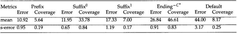
Table 5

Distribution of the error rate and coverage in the cascading guesser.

Metrics Prefix Suffix ° Suffix 1 Ending -c* Default

Error Coverage Error Coverage Error Coverage Error Coverage Error Coverage mean 10.92 5.64 11.95 33.78 17.33 7.00 26.84 46.61 44.00 8.17 s-error 0.95 0.19 0.65 0.84 1.19 0.17 0.91 0.83 3.17 0.25

performed very poorly, having the error rate of 44%. When we compared this distribution to that of the Xerox guesser we saw that the accuracy of the Xerox guesser itself was only about 6.5% lower than that of the cascading guesser 9 and the fact that it could handle 6% fewer u n k n o w n words than the cascading guesser resulted in the increase of incorrect assignments by the default strategy.

There were three types of mistaggings on u n k n o w n words detected in our experiments. Mistagging of the first type occurred when a guesser provided a broader POS-class for an u n k n o w n word than a lexicon would, and the tagger had difficulties with its disambiguation. This was especially the case with the words that were guessed as noun/adjective (NN JJ) but, in fact, act only as one of them (as do, for example, m a n y hyphenated words). Another highly ambiguous group is the

ing

words, which, in general, can act as nouns, adjectives, and gerunds and only direct lexicaliza- tion can restrict the search-space, as in the case of the word

seeing,

which cannot act as an adjective. The second type of mistagging was caused by incorrect assignments by the guesser. Usually this was the case with irregular words such as

cattle

or

data,

which were wrongly guessed to be singular nouns (NN) but in fact were plural nouns (NN8). We also did not include the "foreign word" category (FW) in the set of tags to guess, but this did not do too much harm because these words were very infrequent in the texts. And the third type of mistagging occurred when the word-POS guesser assigned the correct Pos-class to a word but the tagger still disambiguated this class incorrectly. This was the most frequent type of error, which accounted for more than 60% of the mistaggings on u n k n o w n words.

5. C o n c l u s i o n

We have presented a technique for fully automated statistical acquisition of rules that guess possible Pos-tags for words u n k n o w n to the lexicon. This technique does not require specially prepared training data and uses for training a pre-existing general- purpose lexicon and word frequencies collected from a raw corpus. Using such training data, three types of guessing rules are induced: prefix morphological rules, suffix morphological rules, and ending-guessing rules.

Evaluation of tagging accuracy on u n k n o w n words using texts and words unseen at the training phase showed that tagging with the automatically induced cascading guesser was consistently more accurate than previously quoted results known to the author (85%). Tagging accuracy on u n k n o w n words using the cascading guesser was 87.7-88.7%. The cascading guesser outperformed the guesser supplied with the Xerox tagger and the guesser supplied with Brill's tagger both on u n k n o w n proper nouns

[image:16.468.47.433.88.144.2]

(17)

(which is a relatively easy-to-guess category of words) and on the rest of the u n k n o w n words, where it had an advantage of 6.5-8.5.%. When the u n k n o w n words were made known to the lexicon, the accuracy of tagging was 93.6-94.3% which makes the accuracy drop caused by the cascading guesser to be less than 6% in general.

Another important conclusion from the evaluation experiments is that the morphological guessing rules do improve guessing performance. Since they are more accurate than ending-guessing rules they were applied first and improved the precision of the guesses by about 8%. This resulted in about 2% higher accuracy in the tagging of unknown words. The ending-guessing rules constitute the backbone of the guesser and cope with u n k n o w n words without clear morphological structure. For instance, discussing the problem of unknown words for the robust parsing Bod (1995, 84) writes: "Notice that richer, morphological annotation would not be of any help here; the words "return", "stop" and "cost" do not have a morphological structure on the basis of which their possible lexical categories can be predicted." When we applied the ending-guessing rules to these words, the words return and stop were correctly classified as n o u n / v e r b s (NN VB VBP) and only the word cost failed to be guessed by the rules.

The acquired guessing rules employed in our cascading guesser are, in fact, of a standard nature, which, in some form or other, is present in other word-Pos guessers. For instance, our ending-guessing rules are akin to those of Xerox and the morphological rules resemble some rules of Brill's, but ours use more constraints and provide a set of all possible tags for a word rather than a single best tag. The two additional types of features used by Brill's guesser are implicitly represented in our approach as well: One of the Brill schemata checks the context of an u n k n o w n word. In our approach we guess the words using their features only and provide several possi- bilities for a word; then at the disambiguation phase the context is used to choose the right tag. As for Brill's schemata that checks the presence of a particular character in an u n k n o w n word, we capture a similar feature by collecting the ending- guessing rules for proper nouns and hyphenated words separately. We believe that the technique for the induction of the ending-guessing rules is quite similar to that of Xerox 1° or Schmid (1994) but differs in the scoring and pruning methods. The major advantage of the proposed technique can be seen in the cascading application of the different sets of guessing rules and in far superior training data. We use for training a pre-existing general-purpose (as opposed to corpus-tuned) lexicon. This has three advantages:

• the size of the training lexicon is large and does not depend on the size or even the existence of the annotated corpus. This allows for the induction of more rules than from a lexicon derived from an annotated corpus. For instance, the ending guesser of Xerox includes 536 rules whereas our Ending * guesser includes 2,196 guessing rules;

• the information listed in a general-purpose lexicon can be considered to be of better quality than that derived from an annotated corpus, since it lists all possible readings for a word rather than only those that happen to occur in the corpus. We also believe that general-purpose lexicons contain less erroneous information than those derived from annotated corpora;

(18)

• the a m o u n t of w o r k required to prepare the training lexicon is minimal a n d does not require a n y additional m a n u a l annotation.

Our experiments with the lexicon derived from the CELEX lexical database a n d w o r d frequencies derived from the Brown Corpus resulted in guessing rule sets that proved to be domain- a n d corpus-independent (but tag-set-dependent), producing similar results on texts of different origins. An interesting by-product of the proposed rule-induction technique is the automatic discovery of the template morphological rules advocated in Mikheev a n d Liubushkina (1995). The induced morphological guessing rules t u r n e d out to consist mostly of the expected prefixes a n d suffixes of English a n d closely resemble the rules e m p l o y e d b y the ispel| UNIX spell-checker. The rule acquisition a n d evaluation m e t h o d s described here are i m p l e m e n t e d as a m o d u l a r set of c++ a n d AWK tools, a n d the guesser is easily extendible to sublanguage-specific regularities a n d retrainable to n e w tag sets a n d other languages, provided that these languages have affixational morphology.

Acknowledgments

I would like to thank the anonymous referees for helpful comments on an earlier draft of this paper.

References

Baayen, Harald and Richard Sproat. 1995. Estimating lexical priors for

low-frequency morphologically ambiguous forms. Computational Linguistics, 22(3):155-166.

Bod, Rens. 1995. Enriching Linguistics with Statistics: Performance Models of Natural Language. University of Amsterdam ILLC Dissertation Series 1995-14, Academishe Pers, Amsterdam.

Brill, Eric. 1994. Some advances in transformation-based part of speech tagging. In Proceedings of the Twelfth National Conference on Artificial Intelligence (AAAAI-94).

Brill, Eric. 1995. Transformation-based error-driven learning and natural language processing: A case study in part-of-speech tagging. Computational Linguistics, 21(4):543-565.

Burnage, G. 1990. CELEX: A Guide for Users. Nijmegen: Centre for Lexical Information. Church, Kenneth W. 1988. A stochastic parts

program and noun-phrase parser for unrestricted text. In Proceedings of the Second Conference on Applied Natural Language Processing (ANLP-88), pages 136-143.

Cutting, Doug, Julian Kupiec, Jan Pedersen, and Penelope Sibun. 1992. A practical part-of-speech tagger. In Proceedings of the Third Conference on Applied Natural Language Processing (ANLP-92), pages 133-140.

Dermatas, Evangelos and George Kokkinakis. 1995. Automatic stochastic tagging of natural language texts. Computational Linguistics, 21(2):137-164. DeRose, Stephen. 1988. Grammatical

category disambiguation by statistical optimization. Computational Linguistics, 14(1):31-39.

Efron, Bradley and Robert J. Tibshirani. 1993. An Introduction to the Bootstrap. Brace&Co.

Francis, W. Nelson and Henry Kucera. 1982. Frequency Analysis of English Usage: Lexicon and Grammar. Houghton Mifflin, Boston. Hayslett, H.T. 1981. Frequency Analysis of

English Usage Lexicon and Grammar. Heinemann, London.

Kupiec, Julian. 1992. Robust part-of-speech tagging using a hidden Markov model. Computer Speech and Language, pages 225-241.

Lewis, David. 1991. Evaluating text categorization. Speech and Natural

Language: Proceedings of a Workshop Held at Pacific Grove, CA.

Marcus, Mitchell, Mary Ann Marcinkiewicz, and Beatrice Santorini. 1993. Building a large annotated corpus of English: The Penn Treebank. Computational Linguistics, 19(2):313-329.

Mikheev, Andrei. 1996a. Learning part-of-speech guessing rules from lexicon: Extension to non-concatenative operations. In Proceedings of the 16th International Conference on Computational Linguistics (COLING-96), pages 770-775. Mikheev, Andrei. 1996b. Unsupervised

(19)

Mikheev, Andrei and Liubov Liubushkina. 1995. Russian morphology: An

engineering approach. Natural Language Engineering, 1(3):235--260.

Schmid, Helmut. 1994. Part of speech tagging with neural networks. In

Proceedings of the International Conference on Computational Linguistics (COLING-94), pages 172-176.

Tzoukermann, Evelin, Dragomir R. Radev, and William A. Gale. 1995. Combining linguistic knowledge and statistical learning in French part of speech tagging. In Proceedings of the EACL S1GDAT Workshop, pages 51-59.

Voutilainen, Atro. 1995. A syntax-based part-of-speech analyser. In Proceedings of

the Seventh Conference of European Chapter of the Association for Computational Linguistics (EACL-95), pages 157-164.

Weischedel, Ralph, Marie Meteer, Richard Schwartz, Lance Ramshaw, and Jeff Palmucci. 1993. Coping with ambiguity and unknown words through

probabilistic models. Computational Linguistics, 19(2):359-382.

(20)