A Random Text Model for the Generation of
Statistical Language Invariants
Chris Biemann
NLP Dept., University of Leipzig Johannisgasse 26 04103 Leipzig, Germany
Abstract
A novel random text generation model is introduced. Unlike in previous random text models, that mainly aim at producing a Zipfian distribution of word frequencies, our model also takes the properties of neighboring co-occurrence into account and introduces the notion of sentences in random text. After pointing out the defi-ciencies of related models, we provide a generation process that takes neither the Zipfian distribution on word frequencies nor the small-world structure of the neighboring co-occurrence graph as a constraint. Nevertheless, these tions emerge in the process. The distribu-tions obtained with the random generation model are compared to a sample of natu-ral language data, showing high agree-ment also on word length and sentence length. This work proposes a plausible model for the emergence of large-scale characteristics of language without as-suming a grammar or semantics.
1 Introduction
G. K. Zipf (1949) discovered that if all words in a sample of natural language are arranged in de-creasing order of frequency, then the relation be-tween a word’s frequency and its rank in the list follows a power-law. Since then, a significant amount of research in the area of quantitative lin-guistics has been devoted to the question how this property emerges and what kind of processes gen-erate such Zipfian distributions.
The relation between the frequency of a word at rank r and its rank is given by f(r) ∝ r-z, where z is
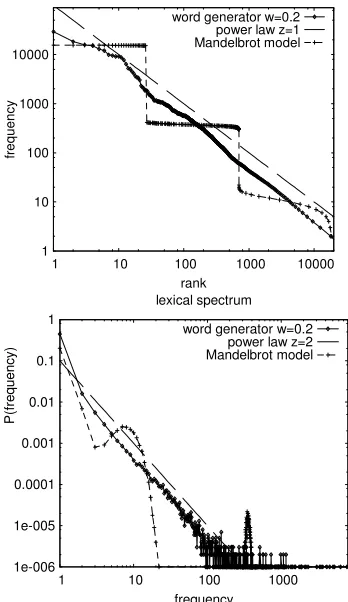
the exponent of the power-law that corresponds to the slope of the curve in a log plot (cf. figure 2). The exponent z was assumed to be exactly 1 by Zipf; in natural language data, also slightly differ-ing exponents in the range of about 0.7 to 1.2 are observed (cf. Zanette and Montemurro 2002). B. Mandelbrot (1953) provided a formula with a closer approximation of the frequency distributions in language data, noticing that Zipf’s law holds only for the medium range of ranks, whereas the curve is flatter for very frequent words and steeper for high ranks. He also provided a word generation model that produces random words of arbitrary average length in the following way: With a prob-ability w, a word separator is generated at each step, with probability (1-w)/N, a letter from an al-phabet of size N is generated, each letter having the same probability. This is sometimes called the “monkey at the typewriter” (Miller, 1957). The frequency distribution follows a power-law for long streams of words, yet the equiprobability of letters causes the plot to show a step-wise rather than a smooth behavior, as examined by Ferrer i Cancho and Solé (2002), cf. figure 2. In the same study, a smooth rank distribution could be obtained by setting the letter probabilities according to letter frequencies in a natural language text. But the question of how these letter probabilities emerge remains unanswered.
Another random text model was given by Simon (1955), which does not take an alphabet of single letters into consideration. Instead, at each time step, a previously unseen new word is added to the stream with a probability a, whereas with probability (1-a), the next word is chosen amongst the words at previous positions. As words with higher frequency in the already generated stream
have a higher probability of being added again, this imposes a strong competition among different words, resulting in a frequency distribution that follows a power-law with exponent z=(1-a). This was taken up by Zanette and Montemurro (2002), who slightly modify Simon’s model. They intro-duce sublinear vocabulary growth by additionally making the new word probability dependent on the time step. Furthermore, they introduce a threshold on the maximal probability a previously seen word can be assigned to for generation, being able to modify the exponent z as well as to model the flat-ter curve for high frequency words. In (Ha et al., 2002), Zipf’s law is extended to words and phrases, showing its validity for syllable-class based languages when conducting the extension.
Neither the Mandelbrot nor the Simon genera-tion model take the sequence of words into ac-count. Simon treats the previously generated stream as a bag of words, and Mandelbrot does not consider the previous stream at all. This is cer-tainly an over-simplification, as natural language exhibits structural properties within sentences and texts that are not grasped by bags of words.
The work by Kanter and Kessler (1995) is, to our knowledge, the only study to date that takes the word order into account when generating random text. They show that a 2-parameter Markov process gives rise to a stationary distribution that exhibits the word frequency distribution and the letter fre-quency distribution characteristics of natural lan-guage. However, the Markov process is initialized such that any state has exactly two successor states, which means that after each word, only two other following words are possible. This certainly does not reflect natural language properties, where in fact successor frequencies of words follow a power-law and more successors can be observed for more frequent words. But even when allowing a more realistic number of successor states, the transition probabilities of a Markov model need to be initialized a priori in a sensible way. Further, the fixed number of states does not allow for infi-nite vocabulary.
In the next section we provide a model that does not suffer from all these limitations.
2 The random text generation model
When constructing a random text generation model, we proceed according to the following
guidelines (cf. Kumar et al. 1999 for web graph generation):
• simplicity: a generation model should reach
its goal using the simplest mechanisms pos-sible but results should still comply to char-acteristics of real language
• plausibility: Without claiming that our
model is an exhaustive description of what makes human brains generate and evolve language, there should be at least a possibil-ity that similar mechanisms could operate in human brains. For a discussion on the sensi-tivity of people to bigram statistics, see e.g. (Thompson and Newport, 2007).
• emergence: Rather than constraining the
model with the characteristics we would like to see in the generated stream, these features should emerge in the process.
Our model is basically composed of two parts that will be described separately: A word generator that produces random words composed of letters and a sentence generator that composes random sentences of words. Both parts use an internal graph structure, where traces of previously gener-ated words and sentences are memorized. The model is inspired by small-world network genera-tion processes, cf. (Watts and Strogatz 1998, Barabási and Albert 1999, Kumar et al. 1999, Steyvers and Tenenbaum 2005). A key notion is the strategy of following beaten tracks: Letters, words and sequences of words that have been gen-erated before are more likely to be gengen-erated again in the future - a strategy that is only fulfilled for words in Simon’s model.
But before laying out the generators in detail, we introduce ways of testing agreement of our ran-dom text model with natural language text.
2.1 Testing properties of word streams
All previous approaches aimed at reproducing a Zipfian distribution on word frequency, which is a criterion that we certainly have to fulfill. But there are more characteristics that should be obeyed to make a random text more similar to natural lan-guage than previous models:
• Lexical spectrum: The smoothness or
fre-quency. In natural language texts, this distri-bution follows a power-law with an expo-nent close to 2 (cf. Ferrer i Cancho and Solé, 2002).
• Distribution of word length: According to
(Sigurd et al., 2004), the distribution of word frequencies by length follows a variant of the gamma distribution
• Distribution of sentence length: The random
text’s sentence length distribution should re-semble natural language. In (Sigurd et al., 2004), the same variant of the gamma distri-bution as for word length is fit to sentence length.
• Significant neighbor-based co-occurrence:
As discussed in (Dunning 1993), it is possi-ble to measure the amount of surprise to see two neighboring words in a corpus at a cer-tain frequency under the assumption of in-dependence. At random generation without word order awareness, the number of such pairs that are significantly co-occurring in neighboring positions should be very low. We aim at reproducing the number of sig-nificant pairs in natural language as well as the graph structure of the neighbor-based co-occurrence graph.
The last characteristic refers to the distribution of words in sequence. Important is the notion of significance, which serves as a means to distin-guish random sequences from motivated ones. We use the log-likelihood ratio for determining signifi-cance as in (Dunning, 1993), but other measures are possible as well. Note that the model of Kanter and Kessler (1995) produces a maximal degree of 2 in the neighbor-based co-occurrence graph.
As written language is rather an artifact of the most recent millennia then a realistic sample of everyday language, we use the beginning of the spoken language section of the British National Corpus (BNC) to test our model against. For sim-plicity, all letters are capitalized and special char-acters are removed, such that merely the 26 letters of the English alphabet are contained in the sam-ple. Being aware that a letter transcription is in itself an artifact of written language, we chose this as a good-enough approximation, although operat-ing on phonemes instead of letters would be pref-erable. The sample contains 1 million words in
125,395 sentences with an average length of 7.975 words, which are composed of 3.502 letters in av-erage.
2.2 Basic notions of graph theory
As we use graphs for the representation of memory in both parts of the model, some basic notions of graph theory are introduced. A graph G(V,E) consists of a set of vertices V and a set of weighted, directed edges between two vertices E⊂V×V×R with R real numbers. The first vertex
of an edge is called startpoint, the second vertex is called endpoint. A function weight: V×V→R
returns the weight of edges. The indegree (outdegree) of a vertex v is defined as the number of edges with v as startpoint (endpoint). The degree of a vertex is equal to its indegree and outdegree if the graph is undirected, i.e. (u,v,w)∈E
implies (v,u,w)∈E. The neighborhood neigh(v) of
a vertex v is defined as the set of vertices s∈S
where (v,s,weight(v,s))∈E.
The clustering coefficient is the probability that two neighbors X and Y of a given vertex Z are themselves neighbors, which is measured for undirected graphs (Watts and Strogatz, 1998). The amount of existing edges amongst the vertices in the neighborhood of a vertex v is divided by the number of possible edges. The average over all vertices is defined as the clustering coefficient C.
The small-world property holds if the average shortest path length between pairs of vertices is comparable to a random graph (Erdös and Rényi, 1959), but its clustering coefficient is much higher. A graph is called scale-free (cf. Barabási and Albert, 1999), if the degree distribution of vertices follows a power-law.
2.3 Word Generator
∑
∈
=
V v
v weightsum
x weightsum x
P
) (
) ( )
(
. ) , ( )
(
) (
∑
∈
=
y neigh u
u y weight y
weightsum
After the generation of the first letter, the word generator proceeds with the next position. At every position, the word ends with a probability w∈(0,1)
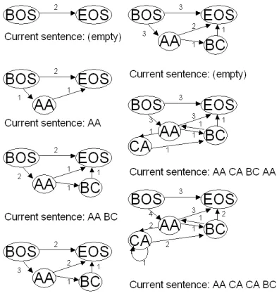
or generates a next letter according to the letter production probability as given above. For every letter bigram, the weight of the directed edge between the preceding and current letter in the letter graph is increased by one. This results in self-reinforcement of letter probabilities: the more often a letter is generated, the higher its weight sum will be in subsequent steps, leading to an increased generation probability. Figure 1 shows how a word generator with three letters A,B,C changes its weights during the generation of the words AA, BCB and ABC.
Figure 1: Letter graph of the word generator. Left: initial state. Right.: State after generating AA, BCB and ABC. The numbers next to edges are edge weights. The probability for the letters for the next step are P(A)=0.4, P(B)=0.4 and P(C)=0.2.
The word end probability w directly influences the average word length, which is given by 1+(1/w). For random number generation, we use the Mersenne Twister (Masumoto and Nishimura, 1998).
The word generator itself does produce a smooth Zipfian distribution on word frequencies and a lexical spectrum following a power-law. Figure 2 shows frequency distribution and lexical spectrum of 1 million words as generated by the word generator with w=0.2 on 26 letters in comparison to a Mandelbrot generator with the same parameters. The reader might note that a similar behaviour could be reached by just setting the probability of generating a letter according to its relative frequency in previously generated words. The graph seems an unnecessary complication for that reason. But retaining the
letter graph with directed edges gives rise to model the sequence of letters for a more plausible morphological production in future extensions of this model, probably in a similar way than in the sentence generator as described in the following section.
As depicted in figure 2, the word generator fulfills the requirements on Zipf’s law and the lexical spectrum, yielding a Zipfian exponent of around 1 and a power-law exponent of 2 for a large regime in the lexical spectrum, both matching the values as observed previously in natural language in e.g. (Zipf, 1949) and (Ferrer i Cancho and Solé, 2002). In contrast to this, the Mandelbrot model shows to have a step-wise rank-frequency distribution and a distorted lexical spectrum. Hence, the word generator itself is already an improvement over previous models as it produces a smooth Zipfian distribution and a lexical spectrum following a power-law. But to comply to the other requirements as given in section 2.1, the process has to be extended by a sentence generator.
1 10 100 1000 10000
1 10 100 1000 10000
fr
e
q
u
e
n
c
y
rank rank-frequency
word generator w=0.2 power law z=1 Mandelbrot model
1e-006 1e-005 0.0001 0.001 0.01 0.1 1
1 10 100 1000
P
(f
re
q
u
e
n
c
y
)
frequency lexical spectrum
[image:4.612.86.265.325.400.2]word generator w=0.2 power law z=2 Mandelbrot model
Figure 2: rank-frequency distribution and lexical spectrum for the word generator in comparison to the Mandelbrot model
[image:4.612.343.517.356.657.2]2.4 Sentence Generator
The sentence generator model retains another di-rected graph, which memorizes words and their sequences. Here, vertices correspond to words and edge weights correspond to the number of times two words were generated in a sequence. The word graph is initialized with a begin-of-sentence (BOS) and an end-of-sentence (EOS) symbol, with an edge of weight 1 from BOS to EOS. When gener-ating a sentence, a random walk on the directed edges starts at the BOS vertex. With a new word probability (1-s), an existing edge is followed from the current vertex to the next vertex according to its weight: the probability of choosing endpoint X from the endpoints of all outgoing edges from the current vertex C is given by
∑
∈
= =
) (
) , (
) , ( )
(
C neigh N
N C weight
X C weight X
word
P .
Otherwise, with probability s∈(0,1), a new
word is generated by the word generator model, and a next word is chosen from the word graph in proportion to its weighted indegree: the probability of choosing an existing vertex E as successor of a newly generated word N is given by
. ) , ( )
(
, ) (
) ( )
(
∑
∑
∈ ∈
= = =
V v
V v
X v weight X
indgw
v indgw
E indgw E
word P
For each sequence of two words generated, the weight of the directed edge between them is in-creased by 1. Figure 3 shows the word graph for generating in sequence: (empty sentence), AA, AA BC, AA, (empty sentence), AA CA BC AA, AA CA CA BC.
During the generation process, the word graph grows and contains the full vocabulary used so far for generating in every time step. It is guaranteed that a random walk starting from BOS will finally reach the EOS vertex. It can be expected that sen-tence length will slowly increase during the course of generation as the word graph grows and the ran-dom walk has more possibilities before finally ar-riving at the EOS vertex. The sentence length is influenced by both parameters of the model: the word end probability w in the word generator and the new word probability s in the sentence genera-tor. By feeding the word transitions back into the generating model, a reinforcement of previously
[image:5.612.327.525.109.326.2]generated sequences is reached. Figure 4 illustrates the sentence length growth for various parameter settings of w and s.
Figure 3: the word graph of the sentence generator model. Note that in the last step, the second CA was generated as a new word from the word gen-erator. The generation of empty sentences happens frequently. These are omitted in the output.
1 10 100
10000 100000 1e+006
a
v
g
.
s
e
n
te
n
c
e
l
e
n
g
th
text interval sentence length growth
w=0.4 s=0.08 w=0.4 s=0.1 w=0.17 s=0.22 w=0.3 s=0.09 x^(0.25);
Figure 4: sentence length growth, plotted in aver-age sentence length per intervals of 10,000 sen-tences. The straight line in the log plot indicates a polynomial growth.
After having defined our random text genera-tion model, the next secgenera-tion is devoted to testing it according to the criteria given in section 2.1. 3 Experimental results
To measure agreement with our BNC sample, we generated random text with the sentence generator using w=0.4 and N=26 to match the English aver-age word length and setting s to 0.08 for reaching a comparable sentence length. The first 50,000 sen-tences were skipped to reach a relatively stable sentence length throughout the sample. To make the samples comparable, we used 1 million words totaling 125,345 sentences with an average sen-tence length of 7.977.
3.1 Word frequency
The comparison between English and the sentence generator w.r.t the rank-frequency distribution is depicted in figure 5.
Both curves follow a power-law with z close to 1.5, in both cases the curve is flatter for high fre-quency words as observed by Mandelbrot (1953). This effect could not be observed to this extent for the word generator alone (cf. figure 2).
1 10 100 1000 10000
1 10 100 1000 10000
fr
e
q
u
e
n
c
y
rank rank-frequency
[image:6.612.342.509.141.288.2]sentence generator English power law z=1.5
Figure 5: rank-frequency plot for English and the sentence generator
3.2 Word length
While the word length in letters is the same in both samples, the sentence generator produced more words of length 1, more words of length>10 and less words of medium length. The deviation in sin-gle letter words can be attributed to the writing system being a transcription of phonemes and few phonemes being expressed with only one letter.
However, the slight quantitative differences do not oppose the similar distribution of word lengths in both samples, which is reflected in a curve of simi-lar shape in figure 6 and fits well the gamma dis-tribution variant of (Sigurd et al., 2004).
1 10 100 1000 10000 100000
1 10
fr
e
q
u
e
n
c
y
length in letters word length
sentence generator English gamma distribution
Figure 6: Comparison of word length distributions. The dotted line is the function as introduced in (Sigurd et al., 2004) and given by f(x) ∝x1.5⋅0.45x.
3.3 Sentence length
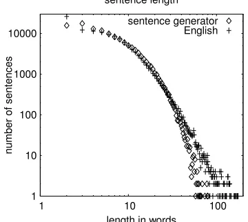
The comparison of sentence length distribution shows again a high capability of the sentence gen-erator to model the distribution of the English sample. As can be seen in figure 7, the sentence generator produces less sentences of length>25 but does not show much differences otherwise. In the English sample, there are surprisingly many two-word sentences.
1 10 100 1000 10000
1 10 100
n
u
m
b
e
r
o
f
s
e
n
te
n
c
e
s
length in words sentence length
[image:6.612.341.521.469.630.2]sentence generator English
Figure 7: Comparison of sentence length distribu-tion.
3.4 Neighbor-based co-occurrence
The significant neighbor-based co-occurrence graph contains all words as vertices that have at least one co-occurrence to another word exceeding a certain significance threshold. The edges are un-directed and weighted by significance. Ferrer i Cancho and Solé (2001) showed that the neighbor-based co-occurrence graph of the BNC is scale-free and the small-world property holds.
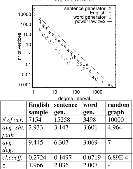
For comparing the sentence generator sample to the English sample, we compute log-likelihood statistics (Dunning, 1993) on neighboring words that at least co-occur twice. The significance threshold was set to 3.84, corresponding to 5% error probability when rejecting the hypothesis of mutual independence. For both graphs, we give the number of vertices, the average shortest path length, the average degree, the clustering coeffi-cient and the degree distribution in figure 8. Fur-ther, the characteristics of a comparable random graph as defined by (Erdös and Rényi, 1959) are shown.
0.001 0.01 0.1 1 10 100 1000 10000
1 10 100 1000
n
r
o
f
v
e
rt
ic
e
s
degree interval degree distribution
sentence generator English word generator power law z=2
English sample
sentence gen.
word gen.
random graph # of ver. 7154 15258 3498 10000 avg. sht.
path
2.933 3.147 3.601 4.964
avg. deg.
9.445 6.307 3.069 7
[image:7.612.68.296.345.635.2]cl.coeff. 0.2724 0.1497 0.0719 6.89E-4 z 1.966 2.036 2.007 -
Figure 8: Characteristics of the neighbor-based co-occurrence graphs of English and the generated sample.
From the comparison with the random graph it is clear that both neighbor-based graphs exhibit the
small-world property as their clustering coefficient is much higher than in the random graph while the average shortest path lengths are comparable. In quantity, the graph obtained from the generated sample has about twice as many vertices but its clustering coefficient is about half as high as in the English sample. This complies to the steeper rank-frequency distribution of the English sample (see fig. 5), which is, however, much steeper than the average exponent found in natural language. The degree distributions clearly match with a power-law exponent of 2, which does not confirm the two regimes of different slopes as in (Ferrer i Cancho and Solé 2001). The word generator data produced an number of significant co-occurrences that lies in the range of what can be expected from the 5% error of the statistical test. The degree distribution plot appears shifted downwards about one decade, clearly not matching the distribution of words in sequence of natural language.
Considering the analysis of the significant neighbor-based co-occurrence graph, the claim is supported that the sentence generator model repro-duces the characteristics of word sequences in natural language on the basis of bigrams.
4 Conclusion
In this work we introduced a random text genera-tion model that fits well with natural language with respect to frequency distribution, word length, sen-tence length and neighboring co-occurrence. The model was not constrained by any a priori distribu-tion – the characteristics emerged from a 2-level process involving one parameter for the word gen-erator and one parameter for the sentence genera-tor. This is, to our knowledge, the first random text generator that models sentence boundaries beyond inserting a special blank character at random: rather, sentences are modeled as a path between sentence beginning and sentence end which im-poses restrictions on the words possible at sentence beginnings and endings. Considering its simplicity, we have therefore proposed a plausible model for the emergence of large-scale characteristics of lan-guage without assuming a grammar or semantics. After all, our model produces gibberish – but gib-berish that is well distributed.
impor-tant role in its production, as it emerges when put-ting a monkey in front of a typewriter. Our model does not only explain Zipf’s law, but many other characteristics of language, which are obtained with a monkey that follows beaten tracks. These additional characteristics can be thought of as arti-facts as well, but we strongly believe that the study of random text models can provide insights in the process that lead to the origin and the evolution of human languages.
For further work, an obvious step is to improve the word generator so that it produces morphologi-cally more plausible sequences of letters and to intertwine both generators for the emergence of word categories. Furthermore, it is desirable to embed the random generator in models of commu-nication where speakers parameterize language generation of hearers and to examine, which struc-tures are evolutionary stable (see Jäger, 2003). This would shed light on the interactions between different levels of human communication.
Acknowledgements
The author would like to thank Colin Bannard, Reinhard Rapp and the anonymous reviewers for useful comments.
References
C. Allauzen, M. Mohri, and B. Roark. 2003.
General-ized algorithms for constructing language models. In Proceedings of the 41st Annual Meeting of the Asso-ciation for Computational Linguistics, pp. 40–47
A.-L. Barabási and R. Albert. 1999. Emergence of
scal-ing in random networks. Science, 286:509-512
T. Dunning. 1993. Accurate Methods for the Statistics
of Surprise and Coincidence. Computational
Linguis-tics, 19(1), pp. 61-74
P. Erdös and A. Rényi. 1959. On Random Graphs I.
Publicationes Mathematicae (Debrecen)
R. Ferrer i Cancho and R. V. Solé. 2001. The
small-world of human language. Proceedings of the Royal Society of London B 268 pp. 2261-2266
R. Ferrer i Cancho and R. V. Solé. 2002. Zipf’s law and
random texts. Advances in Complex Systems, Vol.5
No. 1 pp. 1-6
L. Q. Ha, E. Sicilia-Garcia, J. Ming and F.J. Smith. 2002. Extension of Zipf's law to words and phrases. Proceedings of 19th International Conference on
Computational Linguistics (COLING-2002), pp. 315-320.
G. Jäger. 2003. Evolutionary Game Theory and
Linguis-tic Typology: A Case Study. Proceedings of the 14th Amsterdam Colloquium, ILLC, University of Am-sterdam, 2003.
I. Kanter and D. A. Kessler. 1995. Markov Processes:
Linguistics and Zipf’s law. Physical review letters,
74:22
S. R. Kumar, P. Raghavan, S. Rajagopalan and A. Tom-kins. 1999. Extracting Large-Scale Knowledge Bases
from the Web. The VLDB Journal, pp. 639-650
B. B. Mandelbrot. 1953. An information theory of the
statistical structure of language. In Proceedings of the Symposium on Applications of Communications Theory, London
M. Matsumoto and T. Nishimura. 1998. Mersenne Twister: A 623-dimensionally equidistributed
uni-form pseudorandom number generator. ACM Trans.
on Modeling and Computer Simulation, Vol. 8, No. 1, pp.3-30
G. A. Miller. 1957. Some effects of intermittent silence,.
American Journal of Psychology, 70, pp. 311-314
H. A. Simon. 1955. On a class of skew distribution
functions. Biometrika, 42, pp. 425-440
B. Sigurd, M. Eeg-Olofsson and J. van de Weijer. 2004. word length, sentence length and frequency – Zipf
revisited. Studia Linguistica, 58(1), pp. 37-52
M. Steyvers and J. B. Tenenbaum. 2005. The large-scale structure of semantic networks: statistical
analyses and a model of semantic growth. Cognitive
Science, 29(1)
S. P. Thompson and E. L. Newport. 2007. Statistical learning of syntax: The role of transitional probabil-ity. Language Learning and Development, 3, pp. 1-42.
D. J. Watts and S. H. Strogatz. 1998. Collective
dynam-ics of small-world networks. Nature, 393 pp.
440-442
D. H. Zanette and M. A. Montemurro. 2002. Dynamics
of text generation with realistic Zipf distribution. arXiv:cond-mat/0212496
G. K. Zipf. 1949. Human Behavior and the Principle of