Numerical Simulation of Dynamic Wetting Behavior in the Wetting Balance Method

Full text

(1)Materials Transactions, Vol. 43, No. 8 (2002) pp. 1816 to 1820 Special Issue on Lead-Free Electronics Packaging c 2002 The Japan Institute of Metals. Numerical Simulation of Dynamic Wetting Behavior in the Wetting Balance Method Jeong Whan Han1 , Hwang Gu Lee2 and Jae Yong Park3 1. School of Materials Science & Engineering, Assistant Professor, Inha University, Inchon 402-751, Korea School of Materials Science & Engineering, Graduate Student, Inha University, Inchon 402-751, Korea 3 Material Science & Engineering, Post-doctoral Fellow, UTA, Texas 78712, USA 2. Wetting balance test is known to be the most versatile method to evaluate wettability during soldering process, because it provides quantitative information and time dependent wetting behavior. There are many other studies exist related with the wetting force, however, as to wetting time, there are few theoretical backgrounds and mathematical analysis. In this study, the wetting time is focused on a wettability index. The wetting curve, which shows time dependant wetting behavior, is predicted by using computer simulation and compared with oil experiment also, the mechanism of meniscus rise is analyzed. As a result, relationship of calculated and measured wetting curve can be obtained. It is found that the viscosity of a liquid is the major variable that determine the wetting time and wetting rate. (Received February 18, 2002; Accepted June 12, 2002) Keywords: wetting balance method, computer simulation, wetting time, wetting force, wettability, solderability. 1. Introduction Input/output (I/O) requirements for integrated circuit (IC) packages continue to increase with increasing levels of circuit integration, while the package size continues to decrease. Most of interconnections of the package are based on soldering process-joining between Sn based solder materials and Cu(or Ni) substrate. This interconnection process, however, has several problems: toxicity and radioactivity of lead as a solder alloy element, corrosion of substrate by using flux cleaning agents and excessive growth of Sn–Cu intermetallic compound.1–3) Thus, new solder materials and soldering process are required to address the above problems and the solderability becomes a critical property for both developing new solder materials and soldering processes. Wetting balance method has been known to be the most versatile method to evaluate solderability, because it provides quantitative information and time dependent wetting behavior.4–6) By using wetting balance method a wetting balance curve, which shows the relationship of wetting time and wetting force, can be obtained. Young’s and Laplace equation can give analytical solution of wetting force and static meniscus can be predicted using public domain code called “surface evolver”. In the equations surface tension of a solder and contact angle between a solder and a substrate are the key variables which determine the wetting force.7–9) As to the wetting time, three definitions can be used in general: 1) time span returning to the zero force, 2) the point when the measured force reaches 2/3 of the equilibrium wetting force, and 3) time taken to reach the equilibrium wetting force. However, there are few theoretical backgrounds for the wetting test, and the parameters have to be quantified.10) This study focused on the dynamic behavior of the wetting balance method. By using computer simulation of transient fluid motion of a solder, the physical meaning of the wetting time was discussed. For comparisons silicon oil was used for the experimental simulation of a fluid motion of solder. In this simulation, a temperature effect on viscosity and forma-. tion of intermetallics during soldering could not be taken into account. For this purpose time dependent behavior of silicon oil during wetting balance method was simulated, and then, the volume rise above the oil horizon was translated into the wetting force to obtain a wetting curve. 2. Theoretical Background 2.1 Force balance equation In general Young’s equation can be applied to the interface between substrate and solder. γSV − γLS = γLV cos θ. (1). where, γSV , γLS and γLV are surface tension(or interfacial tension) between the substrate and vapor, between liquid solder and the substrate, and between liquid solder and vapor, respectively. θ is an contact angle at the triple point. Then, a contact angle is determined by the surface tension. The equilibrium wetting force (Feq ) can be expressed as follows: Feq = mg − Fb = Pγ cos θ − ρgVim. (2). where, m is mass of solder rise, g is gravity constant, Fb is the buoyancy force, P is periphery of specimen, ρ is density of a solder, and Vim is volume of the sample immersed into the solder. 2.2 Governing equations for calculating fluid flow The following governing transport equations need to be solved. The equations are based on the conservation of total mass and momentum. Mass continuity and momentum equations are shown in eqs. (3) and (4), respectively. ∂ρ + ∇ · (ρV ) = 0 (3) ∂t ∂V ρ = ρg − ∇ p + ∇ · τij (4) ∂t where, ρ is a density of fluid, ∇ is a vector-gradient operator, V is a velocity-vector field, g is a gravity force, p is a pressure.

(2) Numerical Simulation of Dynamic Wetting Behavior in the Wetting Balance Method. specimen. 1817. Specimen. solder. Solder bath. Fig. 2 Mesh generation of computational domain for numerical simulation.. 0.025. and τ is shear stress. In order to treat fluid interface like free surface in this system, a volume of fluid (VOF) function11) is used. This function represents the volume of fluid per unit volume and satisfies the equation ∂F ∂F ∂F +u +v =0 ∂t ∂x ∂y. (5). The interpretation of F depends on the type of problem being solved. In wetting balance system a single fluid with a free surface, F represents the volume fraction occupied by the fluid. Thus fluid exists where F = 1 and void regions correspond to locations where F = 0. Physically, void represent regions filled with a gas whose density is insignificant with respect to the fluid density. In laminar flow condition the wall shear stress is obtained from the equation below; up (6) τw = µ δy where, µ is the dynamic viscosity of fluid, u p is the fluid velocity adjacent to the wall and δy is the distance from the wall. This formula was based on the assumption that the velocity varies linearly with distance from the wall in a laminar flow.12) The solutions of the transport, turbulent and volume of fluid function equations were obtained using the commercial code FLOW-3D.7) The calculations were made in a transientsolution mode. All the computations were performed on a PC with P-II 500 MHz. With a two-dimensional grid containing 12000 cells (X × Y = 150 × 80) in cartesian coordinate system as shown in Fig. 1, a typical simulation took about 24 hours of CPU time. 3. Experimental Procedure Wetting balance tests were performed with SAT-5000 as shown in Fig. 2. Computer control of the wetting balance; acquisition and analysis of data were performed using wetta-. Wetting Force , F/N ·m. -1. Fig. 1. Schematic drawing of wetting balance tester.. 0.020 0.015 0.010 0.005. Measured Calculated. 0.000 -0.005 0. 1. 2. 3. 4. 5. Time , t/s Fig. 3 Wetting balance results of silicon oil at 25◦ C.. bility tester software by Rhesca Co. For the oil experiments on Cu plate, silicon oil from ShinEtsu Chemical was used. The nominal properties at 25◦ C from the manufacturer are: kinematic viscosity of 0.50 cm2 /s (µ = 0.48 g/cm s), density of 0.963 g/cm3 , and surface tension of 0.00208 J/m−2 . Experiments were made on 99.99% pure Cu plate. The Cu plates were 10 mm wide, 0.15 mm thick, and 15 mm high. Experiments were conducted with the oil bath at room temperature. Before immersion in oil, the plates were cleaned with acetone and alcohol. For the wetting balance tests the immersion speed was set at 1 mm/s and the immersion depth was 0.1 mm. 4. Results and Discussion 4.1 Comparison of oil experiment with computer simulation Figure 3 showed the comparison of experimental and calculated results of wetting balance curves using silicon oil. The immersion depth was set at 0 mm and the bath was withdrawn in 2 seconds. A contact angle was set at 17.5◦ . It was seen from Fig. 3 that the calculated result was matched well with the measurement from the beginning of.

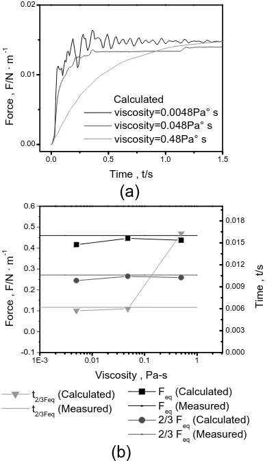
(3) 1818. J. W. Han, H. G. Lee and J. Y. Park Table 1 Comparisons of measured and predicted wetting forces & times.. Calculated Measured Error (%). Feq (N). Rate (N/s). F2/3Feq (N). T2/3Feq (s). Fwd (N). twd (s). 0.0156 0.0160 2.30. 0.0940 0.0912 3.00. 0.0104 0.0106 1.89. 0.1087 0.1167 6.86. 0.0237 0.0228 3.95. 2.312 1.232 87.66. the curve to the level of the equilibrium wetting force. Both the wetting rate, the time to reach an equilibrium state and the equilibrium wetting force showed in good agreements. From these results, it was found that the wetting behavior of silicon oil could be predicted based on the analysis of transport phenomena of the fluid. But the calculated wetting curve during withdrawal stage showed large deviations from the measured one. The moment of detachment of the oil from the specimen (when a maximum withdrawal force is measured) was delayed approximately by 1 second compared to the measurement. This will be explained later. In order to compare the calculated results with the measurement, measured values of the wetting force, the wetting rate and the wetting time were summarized in Table 1. The last row in the table showed the difference in percent error of the calculated wetting indices to the measured one. There were very limited differences in percent error of the equilibrium force (Feq ), wetting rate, two thirds of wetting force (F2/3 ), the time to reach two thirds of wetting force (t2/3 ) and maximum withdrawal force (Fwd ). But the maximum withdrawal time was calculated to be double the measured value. While an initial wetting behavior of the wetting balance curve was quite similar to each other, a large deviation in the withdrawal stage was shown. The reason for this deviation could be explained as follows; during withdrawal oil slides down on the vertical specimen, in this case already oily surface must have an influence upon the measured withdrawal speed of the meniscus. However, in the calculation the withdrawal speed of meniscus could be delayed by bare surface of the specimen. Regarding the maximum withdrawal force less than 4% error was shown and it might not affect on the analysis of the wetting curve. However, further works have to be done on the behavior of wetting time during withdrawal. Figure 4(a) showed the sequential shape changes of the meniscus from the start of wetting to the moment of 0.5 second. As shown in this figure, a contact angle between the oil and the specimen decreases sharply from 90 to 17.5◦ (the time to reach an equilibrium state) and from these results, it was possible to explain that the driving force of wetting was balancing the force at the point of contact angle in equilibrium. Figure 4(b) also showed sequential shape changes of the meniscus during withdrawal. As mentioned before, the wetting balance curve during withdrawal showed a large deviation compared to the measurement and thereby it was difficult to say that the shape change of the meniscus was perfectly simulated. However, from the similar values of the maximum wetting forces by calculations to the measurement, it is expected that the shape change of the meniscus is more or less reasonable. From Fig. 4(b), during oil sliding a contact angle decreased very slowly. But when oil comes to meet the bottom edge of the specimen, a contact angle sharply fell down to zero and moved to the bottom side of the specimen. This. (a). (b). Fig. 4 Calculated meniscus shapes in the initial stage of wetting balance, (a) and in the withdrawal stage of wetting balance, (b).. was similar to the mechanism during withdrawal proposed by Park et al.13, 14) Figure 5 also showed the behavior of the oil remaining on the specimen after the oil detachment. The shape of detached oil (a) changed into sphere type (b → c), followed by a spreading up the specimen (d → f) and finally it formed a thin film on the specimen. These movements caused a weight change of the specimen and then it appeared as fluctuations at the end of the calculated wetting balance curve. 4.2 Effects of oil viscosity Figures 6(a) and (b) showed wetting time and force variations caused by the change in oil viscosity. Since a viscosity is the unique property of the particular liquid, it has a unique certain value of a liquid at a given temperature. The meaning of a change of viscosity in the calculation is to use a different liquid in the measurement. In other words, the test should be conducted with different temperature conditions, contact angles and densities, etc. Practically, it was impossible to change a viscosity of a certain liquid while maintaining all other conditions the same. In this study, however, all other physical properties were assumed to remain the same in order to investigate the pure effect of the viscosity variation on the wetting curve. For the calculations, dynamic viscosities were changed in the range from 0.0048 Pa·s, 0.048 Pa·s and 0.48 Pa·s. Figure 6(a) showed a change of the equilibrium wetting force according to the wetting time. As seen, the beginning part of the wetting balance curve showed a high amplitude at a low viscosity level (µ = 0.0048 Pa·s), whereas those became smoother with increased viscosities. The high amplitude of the wetting curve was caused by the fluctuation of oil surface during withdrawal. In other words, the oil’s shaking triggered by oil rise translated into the steep curve of the.

(4) Numerical Simulation of Dynamic Wetting Behavior in the Wetting Balance Method. a. b. c. t=4.57. t=4.60. t=4.70. t=4.80. t=4.90. t=5.00. f. e. d Fig. 5. Calculated detached oil shape change after the withdrawal.. Force , F/N · m. -1. So far, we have discussed how to evaluate wettability using wetting balance method. The paper was focused on the wetting time using silicon oil to delete complicated conditions, such as heat transfer, interfacial reaction and surface conditions. Oil meniscus during wetting balance test was simulated and the results were translated into conventional wetting curves. A good agreement between measured and calculated wetting curve was obtained. From these, it could be said that the main driving force for liquid rise on the sample was the contact angle. And from the result of viscosity effect on the wetting curve it was found that wetting time was dependent on the viscosity of the liquid. Therefore, it could be inferred from the calculated results that viscosity was one of the possible dominant variable affecting the wettability.. 0.01. Calculated viscosity=0.0048Pa° s viscosity=0.048Pa° s viscosity=0.48Pa° s. 0.00 0.0. 0.5. 1.0. 1.5. Time , t/s. (a) 0.6 0.018. 0.5. 0.015. 0.4. 0.012. 0.3 0.2. 0.009. 0.1. 0.006. 0.0. 0.003. -0.1 1E-3. Time , t/s. -1. fluctuation. But such a rapid curve change disappeared as the viscosity increased. There were no notable changes in equilibrium wetting force by the change of the viscosity but the wetting rates were very different. For example, it was found that the wetting balance curve reached the equilibrium very slowly when the viscosity is 0.48 Pa·s. As shown in Fig. 6(b), there were little changes in equilibrium wetting force and 2/3 wetting force, that is, calculated results were similar to the actual measurements. In the calculation we made so far, the two other variables, surface tension of the liquid and contact angle, which could have an influence upon the wettability, were kept the same. Accordingly, the equilibrium wetting forces remained almost unchanged under different viscosity values. On the contrary, the wetting speed was very sensitive to the viscosity. The calculated value was similar to the actually measured one at 0.0048 Pa·s and 0.048 Pa·s. In other words, wetting time was significantly affected by liquid viscosity. Therefore, it could be inferred from the calculated results that viscosity was one of the dominant variable affecting wetting time in case that equilibrium wetting force was the same. Finally, during testing a wettability of a certain liquid, if several experiments yielded almost similar equilibrium wetting force with different wetting rate or wetting time, we can reason the difference could be caused by the difference of the liquid viscosity. 5. Conclusion. 0.02. Force , F/N · m. 1819. 0.000 0.01. 0.1. This work was supported by INHA UNIVERSITY Research Grant through the special Research Program in 2001.. 1. Viscosity , Pa-s t2/3Feq (Calculated) t2/3Feq (Measured). Acknowledgements. Feq (Calculated) Feq (Measured) 2/3 Feq (Calculated) 2/3 Feq (Measured). (b) Fig. 6 Effects of viscosity on wetting curve, (a) is wetting balance curves with different oil viscosities and (b) is a plot of wetting force against oil viscosity.. REFERENCES 1) E. Wood and K. Nimmo: J. Elec. Mat. 23 (1994) 709–713. 2) N. Koopman, S. Nangalia and V. Rogers: Proc. of IEEE 46th Electronic Components & Technology Conference, (1996) pp. 552–558. 3) J. Kuhmann, H. Hensel, D. Pech, P. Harde and H. Bach: Proc. of IEEE 46th Electronic Components & Technology Conference, (1996) pp. 1088–1092. 4) L. Wilhely: Ann. Phys. 119 (1863) 177. 5) I. Okamoto, T. Takemoto, M. Mizutani and I. Mori: Trans. J. Weld. Res. Inst. 14 (1985) 21. 6) J. Davy and R. Skold: Circuit World, 12 (1985) p. 1..

(5) 1820. J. W. Han, H. G. Lee and J. Y. Park. 7) L. Racz and J. Szekely: EEP Advances in Electronic Packaging, (1993) pp. 1103. 8) W. Liggett and K. Moon and C. Handwerker: Soldering & Surface Mount Technology 9 (1997) 14–21. 9) K. Moon, W. Boettinger, M. Williams, D. Josell, B. Murray, W. Carter and C. Handwerker: J. Elec. Pack. 118 (1996) 174–183. 10) C. Lea and W. Dench: Soldering & Surface Mount Technology 4 (1990). 14–22. 11) C. Hirt and D. Nichols: J. of Computational Physics 39 (1981) 201–225. 12) FLOW-3D User’s Manual, Ver. cv7.7 (2001). 13) J. Park, J. Jung and C. Kang: IEEE Trans. Component Packaging and Technologies 22 (1999) 372–377. 14) J. Y. Park and C. S. Kang and J. P. Jung: J. Elec. Mat. 28 (1999) 1256– 1262..

(6)

No results found